Functional Traits and Local Environmental Conditions Determine Tropical Rain Forest Types at Microscale Level in Southern Ecuador

Abstract

The main objective of this study was to determine the heterogeneity of tropical mountain rain forests along a micro-altitudinal gradient scale, integrating species functional traits in the separation of communities. To achieve this, a forest area of 13 ha in the Biological Reserve of San Francisco was monitored. First, we performed non-metric multidimensional analyses, and afterwards, we looked for correlations between plot altitude and characteristics of the forest (basal area, the number of species, the number of trees ≥20 cm diameter at breast height, per hectare, the forest canopy opening) were associated. To determine which characteristics significantly influence the separation of forest “communities”, we used a multivariate canonical correspondence analysis (CCA). Finally, we carried out the “Four Corners” analysis, combining abundance matrices, traits and environmental variables. We confirmed that the altitude and some associated characteristics are the key factors for the formation of two forest types. In addition, we determined that the inclusion of species functional traits confirms the separation of forest communities, and that elevation and its associated environmental variables function over relatively small areas and scales.

1. Introduction

Tropical forests (TFs) cover 7% of the earth’s surface. Worldwide, 28% of dense forests are tropical mountain forests (TMFs). TFs contain 50% of the world’s forest biomass and are considered the most important natural carbon sinks, with a paramount importance in managing the global climate change [1]. TMF are one of the most diverse and threatened ecosystems on earth; this is especially true for the eastern Andean forests [2]. The last map of global diversity of vascular plant species [3] emphasized the areas of TMFs as the most important hotspots of the world.

Furthermore, TFs generate 36% of the net primary terrestrial production, contributing to the regulation of carbon dioxide (CO₂) concentration in the atmosphere [4,5]. TMFs harbor hydrographic river basins and therefore, they are an essential component in the water regime regulation [6]. Some other functions of these forests are producing wood and non-wood products, catching and storing precipitations and humidity, maintaining the quality of the water, and also reducing erosion and protecting against landslides and floods.

The so-called “Tropical Andes” hotspot includes various types of forests known worldwide for their high diversity [2]. In this type of ecosystem, altitude plays a fundamental role in the distribution of diversity [7]. Several authors recognized that altitude and its associated variables determine richness, floristic composition and structure of the forests in these montane environments [8,9]. In many cases, these variables have a synergic and direct effect on species richness, which generally reaches a peak at approximately 1000 m a.s.l.

In Ecuador, it is estimated that the total number of vascular plant species is between 18,000 and 22,000, one of the highest in the world. Additionally, along the Andes, there is a large number of endemic species restricted to just the middle elevations (900–3000 m) [10]. Despite their global importance, the TMFs in Ecuador are the most threatened type of ecosystems, mainly due to change in land use [11]. The latest reports indicate that already in 2005, 51% of the forest area was lost, with a deforestation rate of 1.7%, which is equivalent to 198,000 ha.

The TMFs distributed along the Andes Real Cordillera in southeastern Ecuador, also termed “montane cloud forest” [12] or “evergreen montane forest” [13], can be partitioned into “mountain rainforest” located between 1800–2800 m a.s.l. and “high mountain evergreen forest” located between 2800 and 3100 m a.s.l. [14]. In both cases, the classification was based on widely used physiognomic patterns of the vegetation in response to macroscale geographic regions. Generally, hierarchical vegetation classification models only work at large scales, and elevation data and species distribution models are too broad to be useful. A classification based on structural parameters, diversity and functional traits of the species is still incipient; this is due to the fact that, at a geographic microscale, the response of the community to the high environmental heterogeneity is much more complicated, and the attempts to classify vegetation into physiognomic distinct categories are not straightforward. In this context, our study is based on the hypothesis that by using functional traits of the species, along with environmental variables, we would be able to delimit the different types of forests present in our study area.

2. Materials and Methods

2.1. General Description of the Study Site

The study was carried out in the Reserva Biologica San Francisco (RBSF) 03°58′ S, 79°04′ W; 1850 m a.s.l. [15], located to the North of Podocarpus National Park (PNP) in Southern Ecuador. RBSF is situated within the eastern cordillera of the Andes [16]. This area is geographically located between Loja and Zamora-Chinchipe provinces (Figure 1).

The soils in the RBSF mainly belong to the order of Inceptisols. At the lower parts of the slopes, Dystrudepts are more frequent, whereas in the upper parts, Humaquepts and Petraquepts dominate [17]. The soils in tropical mountain forests are characterized by thick organic layers, which store large contents of biomass and nutrients [18].

The climate is perhumid, with marked altitudinal gradients in air temperature, humidity and rainfall [19]. The annual mean air temperature ranges from 19.4 °C in the valley to 9.4 °C on the highest mountain tops. The distribution of rainfall is linked to altitude, due to orographic precipitation formation. The average annual rainfall amounts vary between 2300 mm in the valley and 6700 mm on the mountain tops [19].

2.2. Installation of Plots and Forest Inventory

We established 50 × 50 m permanent plots in three different watersheds of the RBSF, named Q2, Q3, and Q5. Twenty plots were installed in Q2 (5 ha), sixteen plots in Q3 (4 ha) and sixteen plots in Q5 (4 ha). In all plots, trees with a diameter at breast height (DBH) ≥ 20 cm were labelled, identified and measured; in addition, 52 central internal plots were installed in each of the large plots, where all the individuals with a DBH of 5–19.9 cm were labelled, identified and measured. Samples from the trees that could not be identified in the field were collected; identification was made by comparison with other botanical specimens collected in the LOJA and HUTPL herbaria of the universities closest to the site.

2.3. Data Acquisition

The data for the floristic and structural analyses were taken directly from the inventories carried out in the field; this allowed, afterwards, the calculation of the average DBH per ha, basal area/ha, average total height of the stand. The canopy openness (defined as the unweighted fraction of unobscured sky) was measured on hemispherical pictures using Gap Light Analyzer software. All terrain data, such as altitude of the midpoint of the plot, inclination and exposure, were acquired in the field and used directly in the environmental matrix. The functional traits of each species used to determine their influence on the division of forest types were: (1) wood density (WD) [20,21,22,23]; (2) average diameter (DBH); (3) growth (annual diametric increase); (4) leaf type; (5) ecological guild [21,23]; (6) dispersal syndrome. Each of these traits is related to different resource use strategies, through acquisitive mechanisms and conservative mechanisms. For example, wood density is related to growth rate, carbon allocation, disease or pest resistance, and primary production [8,20,24]. Leaf type predicts the growth of tropical trees [25] and they present adaptations that allow plants to live in various environmental conditions [26]. As conservative traits, we used the ecological guild or succession type and the “dispersal syndrome”, which is closely related to the relative abundance of species [27] (

Table 1. Functional (conservative and acquisitive) traits, including categories, units and codes used to separate forest types.

Type of Trait	Functional Trait	Categories	Unit
Acquisitive	Wood density	-	g cm3
	Stem density	-	number
	Diametric growth	-	cm year−1
	Leaf type	Simple
		Compound
Conservative	Ecological guild	Shade tolerant
		Partial shade tolerant
		Partial light tolerant
		Light tolerant
		Anemochory
	Dispersal syndrome	Zoochory
		Barochory

).

2.4. Data Analyses

To characterize the forests state in RBSF, structural and floristic parameters were calculated using the following equations (Equations (1)–(5)) [28,29,30,31,32,33,34,35].

$$\mathrm{Relative}\mathrm{Density}\left(\mathrm{RD}\right)=\left(\frac{\mathrm{Individuals}\mathrm{per}\mathrm{species}}{\mathrm{Total}\mathrm{individuals}\mathrm{in}\mathrm{the}\mathrm{plot}}\right)\ast 100$$

(1)

$$\mathrm{Relative}\mathrm{Dominance}\left(\mathrm{RDm}\right)=\left(\frac{\mathrm{Basal}\mathrm{area}\mathrm{per}\mathrm{species}}{\mathrm{Total}\mathrm{Basal}\mathrm{Area}\mathrm{in}\mathrm{the}\mathrm{plot}}\right)\ast 100$$

(2)

$$\mathrm{Relative}\mathrm{Diversity}\left(\mathrm{RDi}\right)=\left(\frac{\#\mathrm{species}\mathrm{per}\mathrm{Family}}{\mathrm{Total}\mathrm{species}}\right)\ast 100$$

(3)

$$\mathrm{Importance}\mathrm{Value}\mathrm{Index}\left(\mathrm{IVI}\right)=(\mathrm{Relative}\mathrm{density}+\mathrm{Relative}\mathrm{Dominance}$$

(4)

$$\mathrm{Shannon}-\mathrm{Wiener}\mathrm{Index}\left({\mathrm{H}}^{\prime }\right)=-{{\displaystyle \sum }}_{\mathrm{i}=1}^{\mathrm{S}}{\mathrm{p}}_{\mathrm{i}}{\mathrm{lnp}}_{\mathrm{i}}$$

(5)

S = number of species (richness);

P_i = proportion of individuals of species with respect to total individuals (i.e., relative abundance of the species) n1/N;

ni = number of individuals of the species.

n1 = number of individuals of the species.

N = number of all the individuals of all the species.

2.5. Statistic Analysis

We generated three matrices. The first consisted of the abundance of individuals in each of the plots, obtained from the post-inventory count. The second matrix consisted of the traits of each of the species involved in the study (

Table 2. CCA model p-values for each variable used.

Variable	Var.N	LambdaA	p	F-Ratio
Altitude	4	0.61	0.001 **	7.09
DBH	7	0.24	0.001 **	3.01
Species	3	0.15	0.001 **	1.76
Trees/ha	2	0.14	0.030 *	1.75
Canopy Openness	8	0.11	0.044 *	1.38
Basal Area/ha	1	0.08	0.279	1.09

Signif. codes: ** 0–0.001; * _0.01.

). Finally, for each plot, both environmental and terrain data were included in the third matrix. These three matrices were used for all statistical analyses of floristic grouping and to measure the influence of functional traits and environmental factors on vegetation grouping.

2.5.1. Non-Metric Multidimensional Scaling (NMDS)

To calculate the resemblance matrix between plots, the Bray–Curtis dissimilarity distance was used. In order to build a dissimilarity matrix between plots, a non-metric multidimensional scaling (NMDS) was performed, to visualize the main environmental factors that influence the grouping of these forest communities. The results were plotted in an NMDS ordination diagram. Values of species abundance, basal area, trees density and environmental variables were fitted onto the first two axes of the NMDS ordination.

The averages at plot level and group level of Shannon diversity index SDI and other characters were compared using a Kruskall–Wallis test between each group assimilable to a vegetation unit. Ordination was performed with the package ‘vegan’ [36] in R software.

2.5.2. Canonical Correspondence Analyses

Canonical correspondence analyses (CCA) were used to test whether the same parameters employed in the correlation analysis influenced the grouping (based on species abundance) of floristic sample plots distributed on the three blocks. This analysis is a multivariate technique that allows representing low-dimensional geometric space proximity between a set of objects influenced by a series of predictor variables. The lambda value corresponds to the eigenvalue of each extracted variable in each axis of the array. F–ratio is calculated using the trace or the sum of all the eigenvalues, while the p value indicates the significance of variables (p ≤ 0.05).

Normally, the CCA involves two matrices: the matrix of dependent variables (e.g., a matrix of sites × species) and the matrix of independent variables (e.g., a matrix of environmental variables). The connection between the two matrices is carried out by means of multivariate regression techniques [37]. Parameters were elevation (m a.s.l.), number of trees ha⁻¹, basal area ha⁻¹, canopy openness (%), average DBH and species richness (total number ha⁻¹).

2.5.3. Correlation

To assess whether there was a significant correlation between the number of trees ha⁻¹, basal area ha⁻¹, DBH ha⁻¹, canopy openness and diversity in terms of Shannon Index and altitudinal gradient, Spearman correlation coefficient was used. If the correlation was significant (r ≥ 0.4; p ≤ 0.05), we considered that the altitude had an impact on the structure and composition of RBSF, determining two or more floristic groups.

2.5.4. Fourth Corner

To complete the analyses that related the characteristics of the forests (growth, DBH, basal area, canopy openness, richness, composition, etc.) and the attitudinal gradient to determine communities or, in this case, determine the types of forests existing in areas and gradients at microscale, we included the functional traits of the species that theoretically were those that respond to altitudinal changes. For this, we used a model-based approach of the fourth-corner analysis [38,39]. This method relates an R matrix of environmental variables to a Q matrix of species traits, by means of an L matrix of species abundance [39]. Depending on the type of variable to relate, a statistic for each pair of traits and environmental variables was computed (Pearson chi-square for two qualitative variables, pseudo-F and correlation ratio for one quantitative and another qualitative variable). Furthermore, a global multivariate statistic linking R and Q arrays was computed as the sum of all statistics mentioned above, in the fourth-corner matrix [40]. The significance of all fourth-corner statistics was tested using permutation model [40]. Here, we used a model where cell values in the L matrix were permuted within each column, testing the null hypothesis that the species were randomly distributed with respect to environmental conditions [41]. All calculus was developed using the “ade4” package [42] in the R software (R Core Team 2021).

3. Results

3.1. Grouping Plots

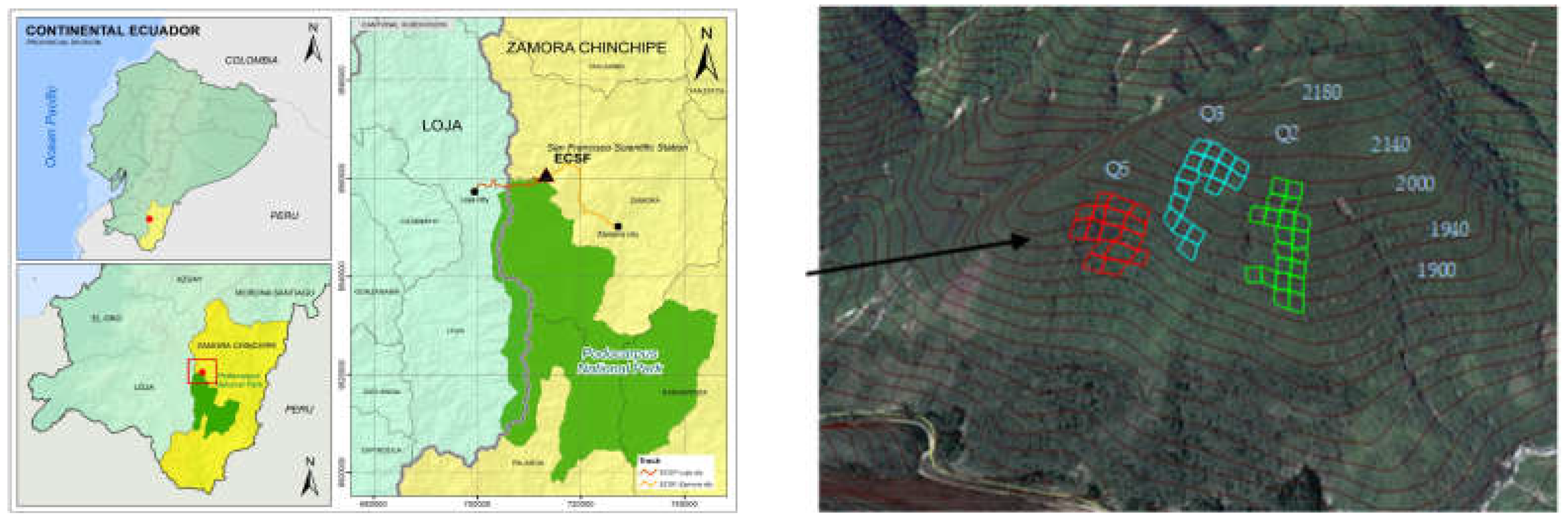
Based on plots of the three sampling sites with floristic similarity and a strong correlation with various attributes of the forest (basal area ha⁻¹, canopy openness, trees ha⁻¹ and alpha diversity), two types of forest could be determined, clearly different in structure and species composition. The spatial distribution of sample plots over the altitudinal gradient implies a change in the structure and diversity of each of the plots. Structural groups were defined based on a correlation between altitude and different attributes of each of the study plots.

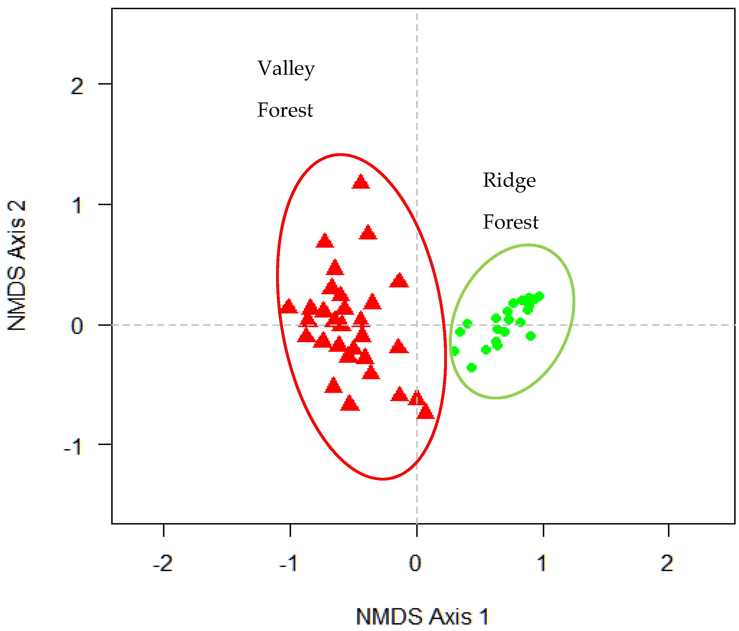
The results of NMDS analysis showed that the sampled plots were divided into two clearly defined groups. The floristic and abundance data used in the matrix formed two groups that we called “forest types”. The first group, named “Valley Forest” (VF), consisted of 15 plots from the Q2 site, and all the plots from the Q5 site. The other group, named “Ridge Forest” (RF), was made up of all the plots of the Q3 site and five plots of the Q2 site (Figure 2).

3.2. Influence of Altitudinal and Structural Parameters on Grouping Communities

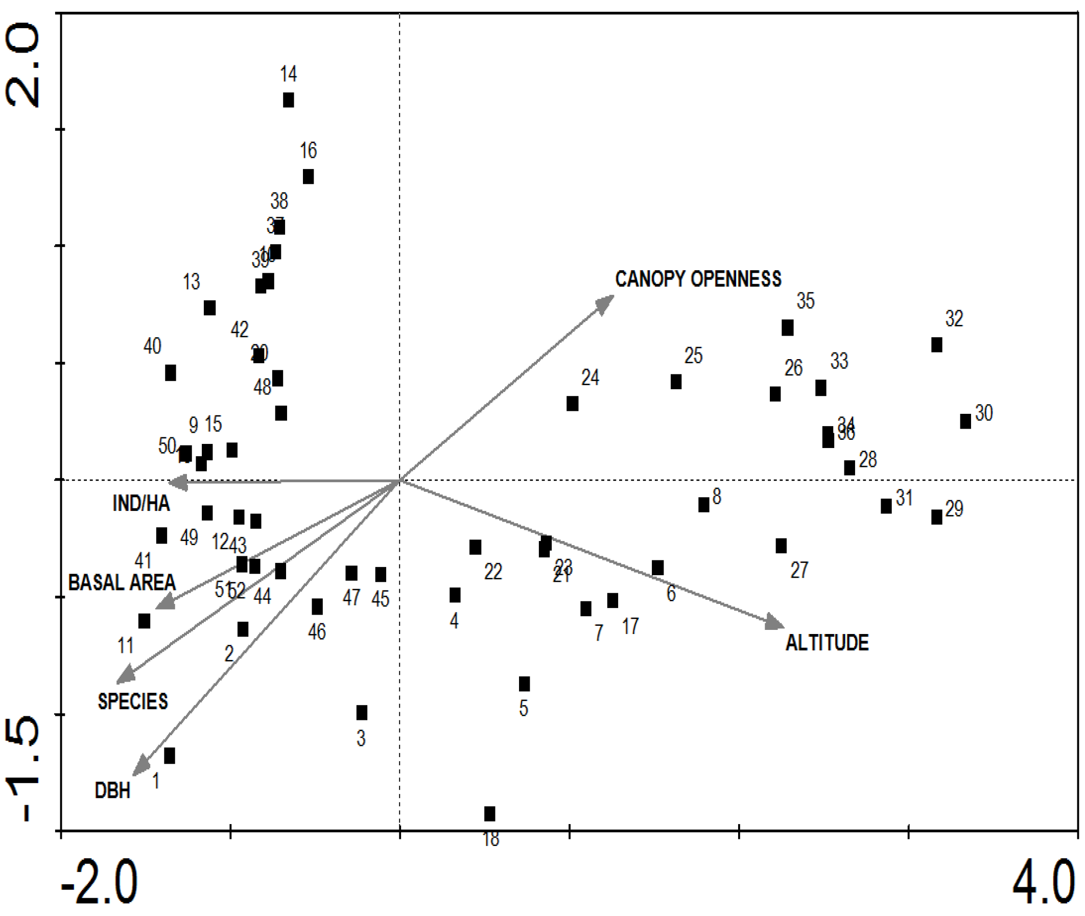
After canonical correspondence Analyses (CCA), altitude was a significative variable in the grouping of the plots, along with basal area and trees per hectare (Figure 3). To a smaller degree, species diversity (expressed as Shannon index) and canopy openness were also factors that determined the grouping. The analyses of the values of the canonical axes explained 18.1% of variance in species data and 84% of its relationship with environmental variables (Table 2). This indicates that the structural and floristic characteristics were the result of the influence of the altitudinal gradient and all environmental variables correlated to this (temperature environmental, precipitation, wind, soil, etc.).

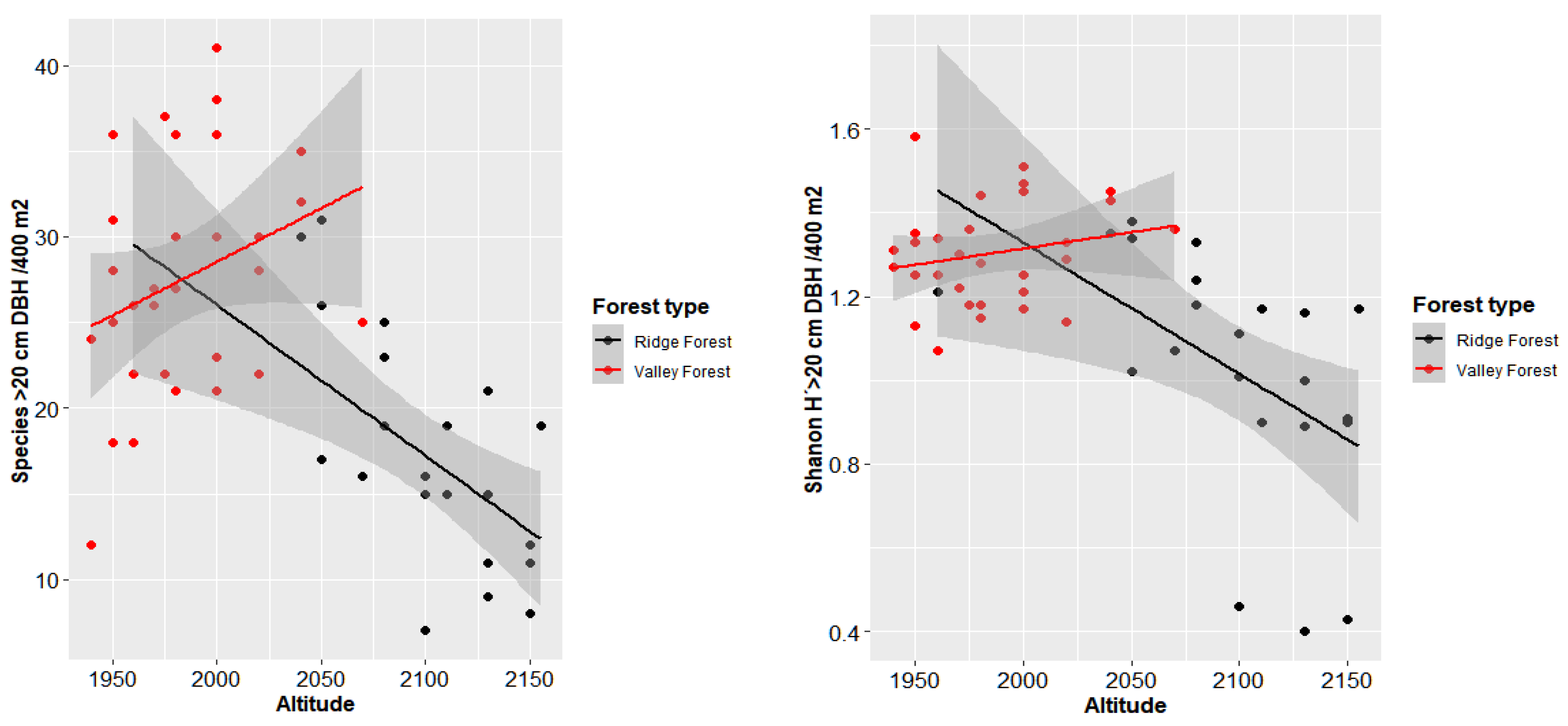
3.3. Correlation between Elevation and Characteristic of Forest

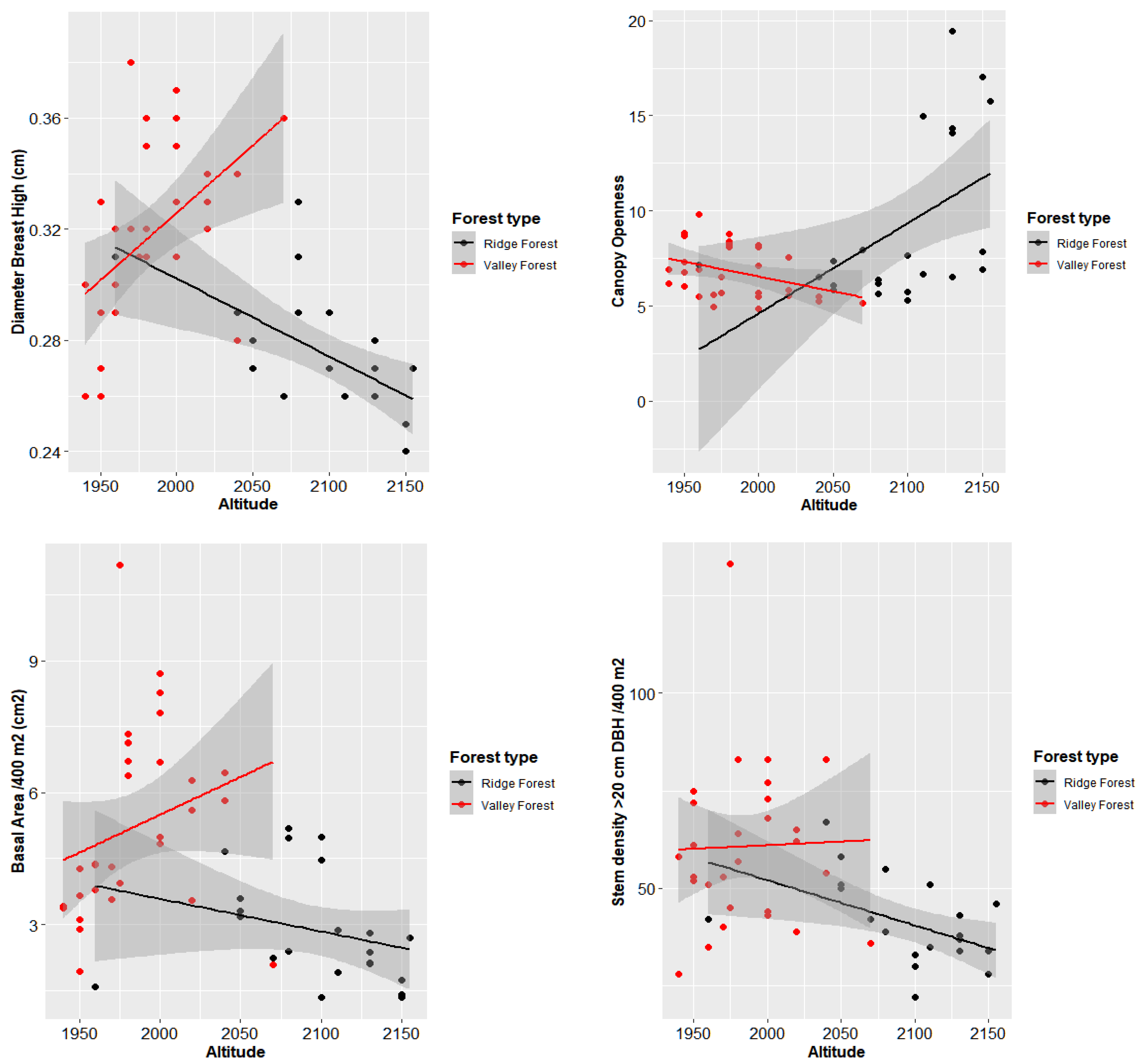
The basal area decreases ad altitude increased; at 1900 m a.s.l., the average basal area can reach 44 m² per hectare (includes only the trees >20 cm DBH). In the plots at 2100 m a.s.l., the average basal area had values of 5 to 14 m² per hectare. The same applied to the number of individuals and to the diversity of the sampled sites. This confirmed the trends found in tropical mountain forests, which means that as altitude increases, the diversity of tree species decreases. Canopy openness was higher with the increasing altitude of the plots. The graphs showed a strong correlation between altitude and variable characteristics of each plot (Figure 4).

The VF is characterized by the presence of Tabebuia chrysantha (Jacq.) G. Nicholson, Cedrela montana Moritz ex Turcz., Inga acreana Harms. and Ficus citrifolia Mill. There are also other species such as Cecropia montana Warb. ex Snethl., Guarea pterorhachis Harms and Heliocarpus americanus L. that are unique to this group.

The RF is characterized by the presence of Podocarpus oleifolius D. Don ex Lamb., Hyeronima moritziana Mull. Arg, Clusia ducuoides Engl., which were species selected as PCT. Other species that characterize the group are Purdiaea nutans Planch., Graffenrieda emarginata (Ruiz and Pav.) and Alchornea grandifolia Triana and Mull Arg.

3.4. Structural Parameters of Floristic Groups

In VF, we encountered 141 species, which belonged to 51 families, while in RF, the diversity was represented by 86 species belonging to 51 families.

Table 3. Values of relative diversity in both forest types.

Valley Forest			Ridge Forest
FAMILIES	Species	Relative Diversity (%)	FAMILIES	# Species	Relative Diversity (%)
Lauraceae	17	12.06	Lauraceae	23	27.7
Moraceae	13	9.22	Euphorbiaceae	7	8.4
Euphorbiaceae	10	7.09	Rubiaceae	5	6
Melastomataceae	9	6.38	Melastomataceae	4	4.8
Meliaceae	9	6.38	Myrtaceae	4	4.8
Cecropiaceae	4	2.84	Clusiaceae	3	3.6
Mimosaceae	4	2.84	Cunnoniaceae	3	3.6
Myrtaceae	4	2.84	Aquifoliaceae	2	2.4
Aquifoliaceae	2	2.13	Arecaceae	2	2.4
Other families (41)	1–2	0.71–2.13	Asteraceae	2	2.4
			Meliaceae	2	2.4
			Mimosaceae	2	2.4
			Moraceae	2	2.4
			Myrsinaceae	2	2.4
			Sapindaceae	2	2.4
			Sapotaceae	2	2.4
			Other families (16)	1	1.2

shows the relative diversity values of the most important families in each of the determined forest types.

Table 4. Values of relative density and relative dominance in the VF.

Valley Forest
Species	Relative Density (%)	Relative Dominance (%)
Cecropia montana	10.52	15.04
Tabebuia chrysantha	4.82	13.53
Guarea pterorhachis	4.46	10.54
Cecropia gabrielis	4.15	5.58
Heliocarpus americanus	3.63	6.13
Hyeronima asperifolia	3.42	7.54
Piptocoma discolor		6.63
Tapirira obtuse		5.57
Sapium glandulosum	3.27	4.58
Miconia quadripora	3.11	4.61
Inga acreana	2.64
Nectandra membranacea	2.54
Other species	0.5–2.64	0.05–3.57

shows the values of density and relative dominance of the most important VF species.

Table 5. Values of relative diversity in both forest types.

Ridge Forest
Species	Relative Density (%)	Relative Dominance (%)
Alchornea grandiflora	11.95	13.37
Alzatea verticillata	10.67	15.03
Clusia ducoides	10.44	10.06
Graffenrieda emarginata	7.77	5.37
Purdiaea nutans	5.57	5.45
Hyeronima moritziana	3.83	3.52
Podocarpus oleifolius	3.71	4.23
Tapirira obtusa	3.36	3.86
Myrcia sp.	3.25	2.35
Dictyocaryum lamarckianum	2.67
Naucleopsis glabra	2.2
Persea ferruginea	1.86
Alchornea pearcei	1.74	2.65
Clusia elliptica	1.74
Nectandra sp.	1.74
Vismia tomentosa	1.62
Persea sp.	1.51
Myrsine coriácea	1.39
Hyeronima asperifolia	1.28
Matayba inelegans	1.16
Other species (58)	0.93–0.12
Other species (76)		0.06–2.27

shows the values of density and relative dominance of the most important RF species.

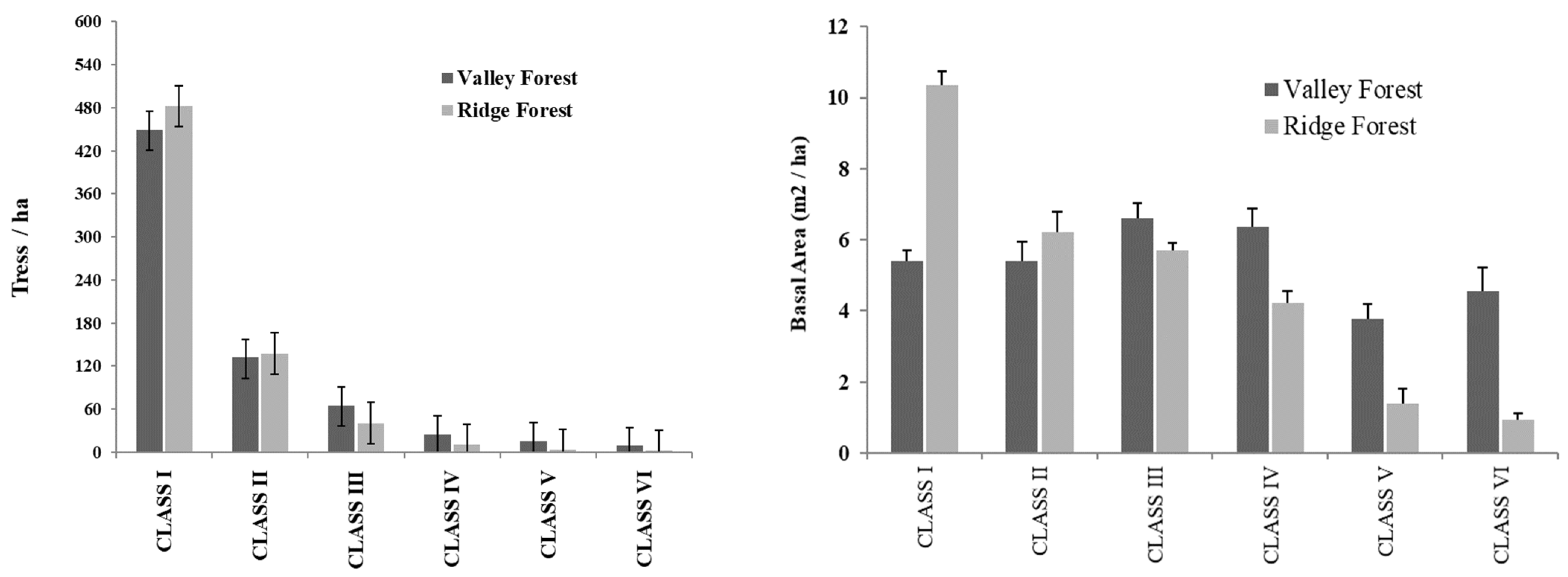
The RF had a total basal area of 54.3 m², with an average of 10.3 ± 3.1 m²ha⁻¹, while the VF had a total basal area of 168.7 m², with an average of 21.8 ± 7.9 m²ha⁻¹, considering only the trees >20 cm DBH.

In the RF, there was a total of 862 individuals > 20 cm DBH and an average of 164.2 ± 35.3 trees ha⁻¹. In the Valley Forest, there was a total of 1933 individuals >20 cm DBH and an average of 248.8 ± 81.4 trees ha⁻¹.

The total basal area of trees in the class 5.1–20 cm DBH in the RF was 3.47 m², which averaged 11.5 ± 3.9 m² ha⁻¹. In VF, the total basal area was 3.7 m² in the class 5.1–20 cm DBH, which means an average of 8.8 ± 3.8 m² ha⁻¹. In RF, there was a total of 443 individuals in the class 5.1–20 cm DBH, with an average of 1464 ± 461.8 trees ha⁻¹. In VF, there was a total of 392 individuals in the class 5.1–20 cm DBH with an average of 906.8 ± 383 ind./ha.

The figures below show the distributions of individuals in all diametric classes in the two forest types (Figure 5).

The structural difference between the two floristic groups was low, but most evident in the first two diametric classes. In RF, there were more individuals per hectare in the first two classes, while in the Valley Forest, there were more individuals per hectare in the higher diameter classes.

In VF, there were more trees in the larger diameter classes, allowing for harvest at a higher intensity. In RF, the small number of large trees suggests lower harvest intensity, the large number of small individuals and the structure of natural regeneration being a typical feature of these forests at this altitude. Regarding the higher number of individuals in lower diameter classes, the RF contained higher basal area values in these classes than the other group (Figure 5).

The diameter distributions of trees in RBSF indicate that the trees were distributed in large quantities in smaller diameter classes and the numbers decreased in a negative exponential way for higher diameter classes. This inverse J-shape distribution type represents a good structure which is typical for natural forests (Figure 5). Each group has its unique species. In the VF, there were 87 exclusive species, representing 47.5% of the total species identified in the study.

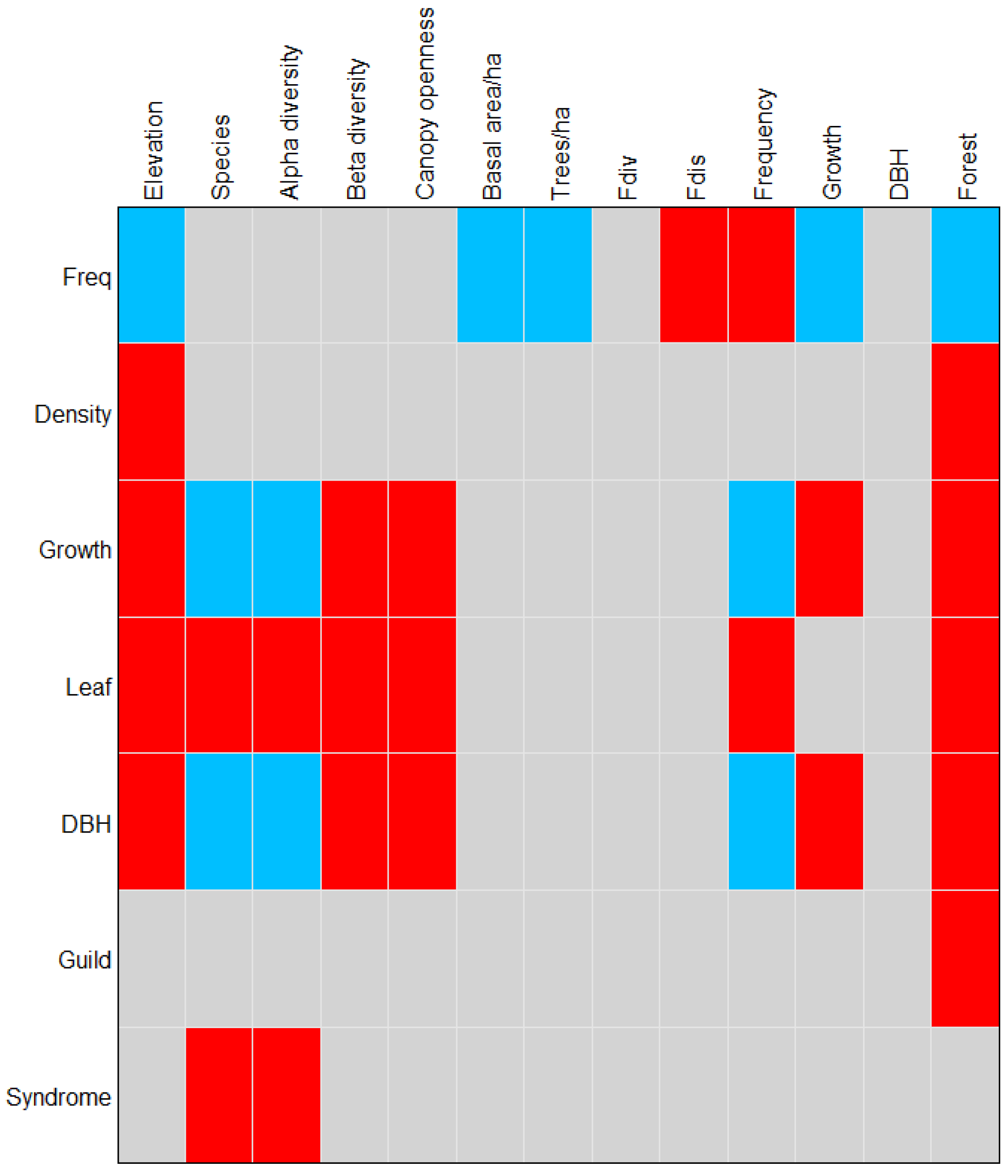
3.5. Functional Traits Influence Forest Separation

The previous results confirmed that the elevation and its associated variables were the main factors that drive the composition and structure of the determined forest types. Likewise, there was a significant correlation at the community level between environmental factors and the plant functional traits as a response to these environmental changes. When incorporating the functional species traits in the determination of the forest types, we found that the conservative traits, such as the dispersal syndrome, were significantly related to the species (p = 0.01) and the alpha diversity of the forest types (p = 0.04). The ecological guild to which the species belongs was strongly related to the elevation (p = 0.05) and the forest type (p = 0.01).

Species acquisitive traits also play a significant role in characterizing forest types. Diametric growth, as the main acquisitive trait, was significantly related to altitude (p = 0.004) and its related variables that, as we observed previously, play an important role in the separation of forest communities.

Both the acquisitive and the conservative traits are important in the conformation of the forest communities; the Four Corner analysis allowed us to include the characteristics of the species that in other analyses went unnoticed, but were significant when classifying the vegetation. Figure 6 shows the correlations between the traits and the environmental variables and

Table 6. p values and type of correlation used in the Four Corner analysis between the functional traits of the species and the environmental variables, based on the species abundance matrix in each of the determined forest plots.

	Traits	Test	Stat. Obs	Std. Obs	Alter	p-Value	p-Value .adj
Altitude	FREC	R	0.103	3.021	two-sided	0.007	0.019 *
AB. HA	FREC	R	0.127	3.716	two-sided	0.001	0.004 **
ARB.HA	FREC	R	−0.126	−3.713	two-sided	0.001	0.004 **
Fdis	FREC	r	0.093	2.609	two-sided	0.019	0.049 *
FREC	FREC	r	0.156	4.515	two-sided	0.001	0.004 **
Growth	FREC	r	−0.129	3.589	two-sided	0.003	0.011 *
Forest	FREC	r	0.102	3.032	two-sided	0.005	0.016 *
Altitude	Density	r	0.140	4.090	two-sided	0.002	0.008 **
Forest	density	r	0.115	3.327	two-sided	0.004	0.014 *
Altitude	Growth	r	0.254	7.673	two-sided	0.001	0.004 **
Species	Growth	r	0.159	4.652	two-sided	0.001	0.004 **
diver.A	Growth	r	0.188	5.568	two-sided	0.001	0.004 **
diver.B	growth	r	0.185	5.449	two-sided	0.001	0.004**
CO	growth	r	0.136	4.073	two-sided	0.001	0.004 **
FREC	Growth	r	0.142	4.132	two-sided	0.002	0.008 **
Forest	Growth	r	0.238	7.201	wo-sided	0.001	0.004 **
Altitude	LEAF	F	5.027	9.009	Greater	0.001	0.004 **
Species	LEAF	F	6.133	1.133	Greater	0.001	0.004 **
diver.A	LEAF	F	4.652	8.274	Greater	0.002	0.008 **
diver.B	LEAF	F	3.064	5.131	greater	0.007	0.019 *
CO	LEAF	F	2.027	3.387	Greater	0.013	0.035 *
FREC	LEAF	F	2.887	4.742	Greater	0.006	0.018 *
DBH	LEAF	F	1.821	3.053	Greater	0.022	0.05.
Forest	LEAF	F	8.230	1.433	Greater	0.001	0.004 **
altitud	DBH	r	0.298	8.638	two-sided	0.001	0.004 **
Species	DBH	r	0.215	6.213	two-sided	0.001	0.004 **
diver. A	DBH	r	0.272	7.984	two-sided	0.001	0.004 **
diver. B	DBH	r	0.262	7.776	two-sided	0.001	0.004 **
CO	DBH	r	0.183	5.216	two-sided	0.001	0.004 **
FREC	DBH	r	0.117	3.438	two-sided	0.004	0.014 *
growth	DBH	r	0.105	3.035	two-sided	0.005	0.016 *
Forest Type	DBH	r	0.275	8.205	two-sided	0.001	0.004 **
Altitude	GUILD	F	8.883	2.810	Greater	0.023	0.05.
Forest	GUILD	F	1.161	4.166	greater	0.007	0.019 *
Species	SYND	F	21.493	5.452	Greater	0.005	0.016 *
diver. A	SYND	F	14.803	3.061	Greater	0.016	0.042 *

Signif. codes: 0 -’ 0.001 ‘**’ 0.01 ‘*’ 0.05 ‘.’ 0.1 ‘ ’ 1.

shows the correlation values between the functional traits of the species and the environmental variables.

4. Discussion

In the proposed model for classification of continental vegetation of Ecuador, Sierra et al. [14] used the regional division of the territory and included the concept of subregions. The hierarchical model divided the regions into sectors, i.e., each region had subregions, and these in turn were divided into sectors, with nesting vegetation physiognomy (Mangrove Forest, Shrubland, Espinar, Savannah, Paramo and Gelidofitia) and other hierarchical criteria such as environmental criteria (dry, wet, fog), phenological criteria (evergreen, deciduous, semi deciduous) and floristic altitudinal levels (lowland, premontane, lower montane, montane, upper montane), determining 62 cover types, 27 on the coast, 24 in the Andes and 11 in the Amazonia.

However, the classification at the plant formation level included large areas that were evidently heterogeneous with respect to key factors, mainly in the composition and structure of the forests. Other authors, such as Valencia et al. [12], called this formation “montane cloud forest” in southeastern Ecuador. This is also known as “Evergreen Montane Forest” [13], using climatic (“cloud”) and functional (“evergreen”) elements in the naming of the formations.

Other classifications proposed altitudinal limits as the main factor in the separation of forests, along with a geomorphological factor [43], asserting that the forest in the southern region of Ecuador can be divided into evergreen lower montane forests (up to 2100–2200 m a.s.l.) and upper montane forests, up to the tree line. Above ~2700 m, a shrub-dominated sub-paramo prevails, where small patches of Elfin Forest, the so-called Ceja Andina, dominate the landscape. Both montane forest types can be subdivided into a lower slope (ravine) forest and an upper slope (ridge) forest [44,45].

A new approach of vegetation classification at smaller scales is based on using variables of structure, taxonomic and functional diversity (traits of the species) and environmental factors (including elevation); as a result, four types of forest can be distinguished by combining different types of classification [8]. For example, [46] studied structural parameters; [47] the floristic trees composition; [48] the bryophytes species composition and [49] making a synopsis of previous studies.

All these studies that classified vegetation using environmental parameters associated with elevation were consistent with the categories of vegetation in the RBSF. Even the topographic variables at smaller scales play an important role in the classification of the vegetation, as demonstrated by the studies carried out by [50] in the same study area and [51] who combine topographic variables and functional features to determine small-scale species association in tropical forests of China.

In the Andean vegetation classifications, the elevation gradient and its associated variables play an essential role in separating forests. This is also true in our case, where elevation works at the microscale, that is, the elevational influence occurs in relatively small areas and over relatively short distances, influencing not only the structure and composition of forests, but also the variation in the composition of traits in vascular plants [52], such as leaf size [53], seed dispersal [54] and wood density [55], which are basically the same traits that we used for our analysis.

Although we did not include topographic variables in our analysis, there were reports that these correlated with vegetation classification, especially at a small scale, and were significant in identifying ecological units that included vegetation structure and composition [56], delimiting forest lowland and montane formations [57]. The topographic variables also affect the functional traits of the species, especially the mass of seeds and the density of the wood [51]; in our case, species wood density was also correlated with altitude and forest type.

Regarding the scale of influence, it should be noted that, although we determined in our study that the influence of elevation and associated variables is also significant at microscales, there are cases in which elevation works at larger scales and its evaluation was also significant [58]. This emphasizes the fact that, in addition to the environmental factors associated with elevation, there are other factors intrinsic to the species that help the differentiation of plant communities.

In a specific approach, altitude and its associated environmental factors are crucial when determining and differentiating forest types. In the VF up to 2050 m a.s.l., the number of trees tends to remain relatively stable, while in the RF, the decline in the number of trees at higher altitudes was evident. This pattern is not strict along the Cordillera de los Andes, but it may be subject to changes in temperature and humidity over relatively short intervals [59].

Finally, when referring to the groups determined by our study, we can indicate that the VF were characterized by lower stem density, but with greater basal areas (tree diameters) and higher canopies compared to the RF, where less tree species were also present. The differences in forest structure are mainly due to the climatic conditions and prevailing soil types [60,61]. At the phytosociological level, the floristic structure and composition of the VF and the RF are coupled to more widely distributed floristic formations, such as the order Alzateetalia verticillatae and Purdiaeaetalia nutantis, respectively [62], which validates the floristic analysis carried out in our study area, by the coincidence of indicator species of each floristic association.

For both floristic groups, the microclimatic and topographic conditions cause the species to find suitable sites and share habitat and topographic preferences of occurrence [50], an argument that also reinforces the grouping of the species present in the forest of the RBSF.

References

1. Saatchi, S.S.; Harris, N.L.; Brown, S.; Lefsky, M.; Mitchard, E.T.; Salas, W.; Zutta, B.R.; Buermann, W.; Lewis, S.L.; Hagen, S. Benchmark. Map of forest carbon stocks in tropical regions across three continents. Proc. Natl. Acad. Sci. USA 2011, 108, 9899–9904. [Google Scholar] [CrossRef] [PubMed] [Green Version]
2. Myers, N.; Mittermeier, R.A.; Mittermeier, C.G.; Da Fonseca, G.A.; Kent, J. Biodiversity hotspots for conservation priorities. Nature 2000, 403, 853–858. [Google Scholar] [CrossRef] [PubMed]
3. Kier, G.; Mutke, J.; Dinerstein, E.; Ricketts, T.H.; Küper, W.; Kreft, H.; Barthlott, W. Global patterns of plant diversity and floristic knowledge. J. Biogeogr. 2005, 32, 1107–1116. [Google Scholar] [CrossRef]
4. Pan, Y.; Birdsey, R.A.; Fang, J.; Houghton, R.; Kauppi, P.E.; Kurz, W.A.; Phillips, O.; Shvidenko, A.; Lewis, S.L.; Canadell, J.G.; et al. A large and persistent carbon sink in the world’s forests. Science 2011, 333, 988–993. [Google Scholar] [CrossRef] [Green Version]
5. Malhi, Y.; Phillips, O.L. Tropical forests and global atmospheric change: A synthesis. Philos. Trans. R. Soc. B 2004, 359, 549–555. [Google Scholar] [CrossRef] [Green Version]
6. FAO. Global Forest Resources Assessment 2005. Main Repor. Progress Towards Sustainable Forest Management; FAO Forestry Papers, FAO: Rome, Italy, 2006; p. 147. [Google Scholar]
7. Cirimwami, L.; Doumenge, C.; Kahindo, J.M.; Amani, C. The effect of elevation on species richness in tropical forests depends on the considered lifeform: Results from an East African mountain forest. Trop. Ecol. 2019, 60, 473–484. [Google Scholar] [CrossRef] [Green Version]
8. Homeier, J.; Breckle, S.W.; Günter, S.; Rollenbeck, R.T.; Leuschner, C. Tree Diversity, Forest Structure and Productivity along Altitudinal and Topographical Gradients in a Species-Rich Ecuadorian Montane Rain Forest. Biotropica 2010, 42, 140–148. [Google Scholar] [CrossRef]
9. Apaza-Quevedo, A.; Lippok, D.; Hensen, I.; Schleuning, M.; Both, S. Elevation, topography, and edge effects drive functional composition of woody plant species in tropical montane forests. Biotropica 2015, 47, 449–458. [Google Scholar] [CrossRef]
10. Valencia, R.; Churchill, S.P.; Balslev, H.; Forero, E.; Luteyn, J.L. Composition and structure of an Andean Forest fragment in eastern Ecuador. In Biodiversity and Conservation of Neotropical Montane Forests. Proceedings of a Symposium, New York Botanical Garden; New York Botanical Garden: New York, NY, USA, 1995. [Google Scholar]
11. Mosandl, R.; Günter, S.; Stimm, B.; Weber, M. Ecuador suffers the highest deforestation rate in South America. In Gradients in a Tropical Mountain Ecosystem of Ecuador; Springer: Berlin/Heidelberg, Germany, 2008. [Google Scholar]
12. Valencia, R.; Cerón, C.; Palacios, W. Las formaciones naturales de la Sierra del Ecuador. In Propuesta Preliminar de un Sistema de Clasificación de Vegetación Para el Ecuador Continental; Sierra, R., Ed.; Proyecto INEFAN/GEF-BIRF and EcoCiencia: Quito, Ecuador, 1999; pp. 81–108. [Google Scholar]
13. Balslev, H.; Øllgaard, B. Mapa de vegetación del sur de Ecuador. In Botánica Austroecuatoriana; Ediciones Abya-Yala: Quito, Ecuador, 2002; pp. 51–64. [Google Scholar]
14. Sierra, R. Propuesta Preliminar de un Sistema de Clasificación de Vegetación Para el Ecuador Continental; Proyecto Inefan/Gef-Birf y Ecociencia: Quito, Ecuador, 1999. [Google Scholar]
15. Ohl, C.; Bussmann, R. Recolonisation of natural landslides in tropical mountain forests of Southern Ecuador. Feddes Repert. 2004, 115, 248–264. [Google Scholar] [CrossRef]
16. Brehm, G.; Homeier, J.; Fiedler, K. Beta diversity of geometrid moths (Lepidoptera: Geometridae) in an Andean montane rainforest. Divers. Distrib. 2003, 9, 351–366. [Google Scholar] [CrossRef]
17. Schrumpf, M.; Guggenberger, G.; Valarezo, C.; Zech, W. Tropical montane rain forest soils. Development and nutrient status along an altitudinal gradient in the south Ecuadorian Andes. Erde 2001, 132, 43–59. [Google Scholar]
18. Wilcke, W.; Yasin, S.; Schmitt, A.; Valarezo, C.; Zech, W. Soils along the altitudinal transect and in catchments. In Gradients in a Tropical Mountain Ecosystem of Ecuador; Springer: Berlin/Heidelberg, Germany, 2008; pp. 75–85. [Google Scholar]
19. Fries, A.; Rollenbeck, R.; Bayer, F.; Gonzalez, V.; Oñate-Valivieso, F.; Peters, T.; Bendix, J. Catchment precipitation processes in the San Francisco valley in southern Ecuador: Combined approach using high-resolution radar images and in situ observations. Meteorol. Atmos. Phys 2014, 126, 13–29. [Google Scholar] [CrossRef]
20. Zanne, A.E.; Lopez-Gonzalez, G.; Coomes, D.A.; Ilic, J.; Jansen, S.; Lewis, S.L.; Chave, J. Global Wood Density Database. Dryad. Identifier. 2009. Available online: http://datadryad.org/handle/10255/dryad.235 (accessed on 23 January 2023).
21. Chave, J.; Coomes, D.A.; Jansen, S.; Lewis, S.L.; Swenson, N.G.; Zanne, A.E. Towards a worldwide wood economics spectrum. Ecol. Lett. 2009, 12, 351–366. [Google Scholar] [CrossRef]
22. MAE. Resultados de la Evaluación Nacional Forestal; Ministerio del Ambiente: Quito, Ecuador, 2014. [Google Scholar]
23. Palacios, W.A. Forest species communities in tropical rain forest of Ecuador. Lyonia 2004, 7, 33–40. [Google Scholar]
24. Osazuwa-Peters, O.L.; Jiménez, I.; Oberle, B.; Chapman, C.A.; Zanne, A.E. Selective logging: Do rates of forest turnover in stems, species composition and functional traits decrease with time since disturbance? A 45 year perspective. For. Ecol. Manag 2015, 357, 10–21. [Google Scholar] [CrossRef] [Green Version]
25. Dos Santos, V.A.H.F.; Ferreira, M.J. Are photosynthetic leaf traits related to the first-year growth of tropical tree seedlings? A light-induced plasticity test in a secondary forest enrichment planting. For. Ecol. Manag 2020, 460, 117900. [Google Scholar] [CrossRef]
26. Wang, C.; Zhou, J.; Xiao, H.; Liu, J.; Wang, L. Variations in leaf functional traits among plant species grouped by growth and leaf types in Zhenjiang, China. J. For. Res. 2017, 28, 241–248. [Google Scholar] [CrossRef]
27. Jara-Guerrero, A.; De la Cruz, M.; Méndez, M. Seed dispersal spectrum of woody species in south Ecuadorian dry forests: Environmental correlates and the effect of considering species abundance. Biotropica 2011, 43, 722–730. [Google Scholar] [CrossRef] [Green Version]
28. Aguirre Calderón, Ó.A.; Jiménez Pérez, J.; Kramer, H.; Akça, A. Análisis estructural de ecosistemas forestales en el Cerro del Potosí, Nuevo León, México. Ciencia 2003, 6. [Google Scholar]
29. Cerón, C. Manual de Botánica Ecuatoriana, Sistemática y Métodos de Estudio, Escuela de Biología; Universidad Central del Ecuador: Quito, Ecuador, 1993. [Google Scholar]
30. Madsen, J.E.; Øllgaard, B. Floristic composition, structure, and dynamics of an upper montane rain forest in Southern Ecuador. Nord. J. Bot. 1994, 14, 403–423. [Google Scholar] [CrossRef]
31. Madsen, J.E. Floristic Composition, Structure and Dynamics of an Upper Montane Rain Forest in Southern Ecuador. Ph.D. Thesis, Botanical Institute of Aarhus University, Aarhus, Denmark, 1991. [Google Scholar]
32. Finol, U.H.; Finol, U.H. Estudio fitosociológico de las unidades 2 y 3 de la Reserva Forestal de Caparo, Estado Barinas. Acta Botánica Venez. 1976, 11, 15–103. [Google Scholar]
33. Galindo, R.; Betancur, J.; Cadena, J.J. Estructura y composición florística de cuatro bosques andinos del santuario de flora y fauna Guanentá-Alto río Fonce, cordillera oriental colombiana. Caldasia 2003, 25, 313–335. [Google Scholar]
34. Mori, S.A.; Boom, B.M.; de Carvalino, A.M. Ecological importance of Myrtaceae in an eastern Brazilian wet forest. Biotropica 1983, 15, 68–70. [Google Scholar] [CrossRef]
35. Magurran, A.E. Why diversity? In Ecological Diversity and Its Measurement; Springer: Dordrecht, The Netherlands, 1988; pp. 1–5. [Google Scholar]
36. Petchey, O.L.; Gaston, K.J. Functional diversity: Back to basics and looking forward. Ecol. Lett. 2006, 9, 741–758. [Google Scholar] [CrossRef]
37. Cayuela, L. Una Introduccion a R. EcoLab, Centro Andaluz de Medio Ambiente; Universidad de Granada: Granada, Spain, 2010; 109p. [Google Scholar]
38. Legendre, P.; Galzin, R.; Harmelin-Vivien, M.L. Relating behavior to habitat: Solutions to the fourth-corner problem. Ecology 1997, 78, 547–562. [Google Scholar] [CrossRef]
39. Dray, S.; Choler, P.; Dolédec, S.; Peres-Neto, P.R.; Thuiller, W.; Pavoine, S.; ter Braak, C.J. Combining the fourth-corner and the RLQ methods for assessing trait responses to environmental variation. Ecology 2014, 95, 14–21. [Google Scholar] [CrossRef] [Green Version]
40. Dray, S.; Legendre, P. Testing the species traits–environment relationships: The fourth-corner problem revisited. Ecology 2008, 89, 3400–3412. [Google Scholar] [CrossRef]
41. Aubin, I.; Ouellette, M.H.; Legendre, P.; Messier, C.; Bouchard, A. Comparison of two plant functional approaches to evaluate natural restoration along an old-field–deciduous forest chronosequence. J. Veget. Sci. 2009, 20, 185–198. [Google Scholar] [CrossRef]
42. Chessel, D.; Dufour, A.B.; Dray, S. Analysis of Ecological Data: Exploratory and Euclidean Methods in Environmental Sciences. Version 1.4-14. 2 October 2010; Lyon, France1: 4, 11. 2009. Available online: http://pbil.univ-lyon1.fr/ADE-4/ade4-html/00Index.html (accessed on 23 January 2023).
43. Homeier, J.; Leuschner, C.; Bräuning, A.; Cumbicus, N.L.; Hertel, D.; Martinson, G.O.; Spannl, S.; Veldkamp, E. Effects of nutrient addition on the productivity of montane forests and implications for the carbon cycle. In Ecosystem Services, Biodiversity and Environmental Change in a Tropical Mountain Ecosystem of South Ecuador; Springer: Berlin/Heidelberg, Germany, 2013; pp. 315–329. [Google Scholar]
44. Werner, F.A.; Homeier, J. Is tropical montane forest heterogeneity promoted by a resource-driven feedback cycle? Evidence from nutrient relations, herbivory and litter decomposition along a topographical gradient. Funct. Ecol. 2015, 29, 430–440. [Google Scholar] [CrossRef]
45. Paulick, S.; Dislich, C.; Homeier, J.; Fischer, R.; Huth, A. The carbon fluxes in different successional stages: Modelling the dynamics of tropical montane forests in South Ecuador. For. Ecosyst. 2017, 4, 5. [Google Scholar] [CrossRef] [Green Version]
46. Paulsch, A. Development and Application of a Classification System for Undisturbed and Disturbed Tropical Montane Forests Based on Vegetation Structure. Ph.D. Dissertation, Fakultat fur Biologie, Chemie und Geowissenschaften der Universitat Bayreuth, Bayreuth, Germany, 2002. [Google Scholar]
47. Homeier, J. Baumdiversität, Waldstruktur und Wachstumsdynamik Zweier-Tropischer Bergregenwälder in Ecuador und Costa Rica. Ph.D. Thesis, University of Bielefeld, Bielefeld, Germany, 2004. [Google Scholar]
48. Parolly, G.; Kürschner, H. Ecosociological studies in Ecuadorian bryophyte communities. V. Syntaxonomy, life forms and life strategies of the bryophyte vegetation on decaying wood and tree bases in S Ecuador. Nova Hedwigia 2005, 81, 1–36. [Google Scholar] [CrossRef]
49. Homeier, J.; Werner, F.A.; Gradstein, S.R.; Breckle, S.; Richter, M. Potential vegetation and floristic composition of Andean forests in South Ecuador, with a focus on the RBSF. Ecol. Stud. 2008, 198, 87. [Google Scholar]
50. Kuebler, D.; Hildebrandt, P.; Günter, S.; Stimm, B.; Weber, M.; Mosandl, R.; Muñoz, J.; Cabrera, O.; Aguirre, N.; Zeilinger, J.; et al. Assessing the importance of topographic variables for the spatial distribution of tree species in a tropical mountain forest. Erdkunde 2016, 70, 19–47. [Google Scholar] [CrossRef]
51. Liu, J.; Yunhong, T.; Slik, J.F. Topography related habitat associations of tree species traits, composition and diversity in a Chinese tropical forest. For. Ecol. Manag. 2014, 330, 75–81. [Google Scholar] [CrossRef]
52. Duivenvoorden, J.F.; Cuello, A.N. Functional trait state diversity of A ndean forests in Venezuela changes with altitude. J. Veg. Sci. 2012, 23, 1105–1113. [Google Scholar] [CrossRef]
53. Malhado, A.C.M.; Malhi, Y.; Whittaker, R.J.; Ladle, R.J.; ter Steege, H.; Phillips, O.L.; Butt, N.; Aragão, L.E.O.C.; Quesada, C.A.; Araujo-Murakami, A.; et al. Spatial trends in leaf size of Amazonian rainforest trees. Biogeosciences 2009, 6, 1563–1576. [Google Scholar] [CrossRef] [Green Version]
54. Antonio Vazquez, G.J.; Givnish, T.J. Altitudinal gradients in tropical forest composition, structure, and diversity in the Sierra de Manantlán. J. Ecol. 1998, 86, 999–1020. [Google Scholar]
55. Chave, J.; Muller-Landau, H.C.; Baker, T.R.; Easdale, T.A.; Steege, H.T.; Webb, C.O. Regional and phylogenetic variation of wood density across 2456 neotropical tree species. Ecol App. 2006, 16, 2356–2367. [Google Scholar] [CrossRef] [Green Version]
56. Körner, C.; Paulsen, J. A world‐wide study of high altitude treeline temperatures. J. Biogeogr. 2004, 31, 713–732. [Google Scholar]
57. Jadán, O.; Donoso, D.A.; Cedillo, H.; Bermúdez, F.; Cabrera, O. Floristic groups, and changes in diversity and structure of trees, in tropical montane forests in the Southern Andes of Ecuador. Diversity 2021, 13, 400. [Google Scholar]
58. Treiber, J.; von Wehrden, H.; Zimmermann, H.; Welk, E.; Jäger, E.J.; Ronnenberg, K.; Wesche, K. Linking large-scale and small-scale distribution patterns of steppe plant species—An example using fourth-corner analysis. Flora 2020, 263, 151553. [Google Scholar] [CrossRef]
59. Malizia, A.; Blundo, C.; Carilla, J.; Acosta, O.O.; Cuesta, F.; Duque, A.; Aguirre, N.; Aguirre, Z.; Ataroff, M.; Baez, S.; et al. Elevation and latitude drive structure and tree species composition in Andean forests: Results from a large-scale plot network. PLoS ONE 2020, 15, e0231553. [Google Scholar] [CrossRef] [PubMed] [Green Version]
60. Moser, G.; Leuschner, C.; Hertel, D.; Graefe, S.; Soethe, N.; Iost, S. Elevation effects on the carbon budget of tropical mountain forests (S Ecuador): The role of the belowground compartment. Glob. Chang. Biol. 2011, 17, 2211–2226. [Google Scholar] [CrossRef] [Green Version]
61. Dislich, C.; Huth, A. Modelling the impact of shallow landslides on forest structure in tropical montane forests. Ecol. Model 2012, 239, 40–53. [Google Scholar] [CrossRef]
62. Bussmann, R.W. Los bosques montanos de la Reserva Biológica San Francisco (Zamora-Chinchipe, Ecuador)—Zonación de la vegetación y regeneración natural. Lyonia 2003, 3, 57–72. [Google Scholar]
Figure 1. Location of Reserva Biologica San Francisco and Podocarpus National Park. Blocks and plots ubication.
Diversity 15 00420 g001
Figure 2. Non-metric multidimensional scaling analysis of species composition for the samples (plots).
Diversity 15 00420 g002
Figure 3. Biplot showing the ordination of 52 sample plots, points show the grouping and the vectors indicate the variables that mostly influenced the grouping.
Diversity 15 00420 g003
Figure 4. Changes of diversity and structure in altitudinal gradient. Significant correlations (p < 0.05) are shown in regression line. For all tests, n = 52 plots.
Diversity 15 00420 g004aDiversity 15 00420 g004b
Figure 5. Average basal area ha−1 and trees ha−1 by diameter classes on each forest type.
Diversity 15 00420 g005
Figure 6. The relationship between trees functional traits and habitat variables. Colors represent the strength of interactions (shading) and their direction. Red indicates a positive association and blue indicates a negative association. The scale bar indicates the values of fourth-corner coefficients. Elev elevation, TD tree density. See Table 2 for definition of traits.
Diversity 15 00420 g006