A Biosensor Based on Bound States in the Continuum and Fano Resonances in a Solid–Liquid–Solid Triple Layer

Abstract

We propose a simple solid–liquid–solid triple layer biosensor platform based on bound states in the continuum (BICs) and Fano resonances to detect the acoustic properties of liquids and apply the method to a mixture of water and albumin with various concentrations. The solid–liquid–solid triple layer is composed of an epoxy as a solid layer and an albumin–water mixture as a liquid layer, and the entire system is immersed in water. In this work, we show that the structure exhibits a high sensitivity (S), quality factor (Q), and figure of merit (FOM) with a better detection limit (DL) in the vicinity of the BICs where the transmission spectra exhibit Fano resonances. The Fano resonances shift towards high frequencies as the concentration increases. The detection limit can reach very small values for a small albumin concentration ($4.7\%$). In addition, for a given concentration and layer thickness of the sensing material, we show the effect of the incidence angle on the efficiency of the sensor in terms of the sensitivity and quality factor. The proposed structure can be designed from low-cost material and can be used as a sensor to detect different types of liquids and gases as well.

1. Introduction

One of the most prominent applications of acoustic waves is their use in the sensing field. The interest in sensors based on resonant systems has increased considerably over the past decade [1,2]. Recently, the interest of studying and developing sensors, particularly biosensors, has attracted attention in numerous areas, such as optical [3,4,5,6,7,8] and acoustical [9,10,11,12,13,14] biosensors. Biosensors based on surface plasmon resonances are the most commonly used for protein detection in optics [15,16], but they remain relatively expensive. Thus, the increasing interest in developing biosensors based on phononic crystals (PCs) with a high sensitivity has become a competitive alternative to optical biosensors [14,17]. On the other hand, acoustic biosensors use two types of acoustic waves as a detection mechanism to obtain biophysical and medical information through the sensing material employed [18,19]: bulk acoustic waves (BAW) and surface acoustic waves (SAW). In BAW sensors [1,20,21], the acoustic wave propagates throughout the crystal; hence, the sensitivity is linked to the ratio of the increasing mass to the mass of the entire sensing system. In SAW devices [22,23], the acoustic wave propagates parallel and in the vicinity of the surface, so the sensitivity becomes affected by the ratio of the concentration mass to the mass of the sensing material where the acoustic energy is confined at the surface of the sensor. In addition to BAW and SAW sensors, there are other sensors based on the presence of a cavity by creating a defect inside an arrangement of periodic systems [24,25,26]. When a wave propagates through the cavity medium, it responds to the speed of sound and the density of the sensing material, leading to different resonance peaks for specific cavity properties.

One of the most important features of biosensor devices lies in its sensing in detecting a liquid with its physical properties according to the concentration. In this regard, Oseev et al. [24] presented a phononic crystal (PC) sensor with a cavity that determines gasoline properties. Zubstov et al. [25] used a new PC sensor with a normal incidence of sound to measure the concentration of a liquid mixture. Mukhin et al. [26] studied theoretically and experimentally a PC liquid sensor based on narrow band composite solid–liquid structures by varying the inserted liquid. As mentioned above, in most PC liquid sensors, the mechanism lies in creating a cavity inside a periodic structure, thus breaking the periodicity of PCs and generating a resonant peak inside the band gap [2,25,26,27,28].

In this paper, we present a biosensor based on a simple solid–liquid–solid triple layer supporting bound states in the continuum (BICs) and Fano resonances. Recently, we have demonstrated theoretically [29] and verified experimentally [30] the existence of BICs and Fano resonances in such a triple layer embedded in water. BICs are considered non-radiative states with corresponding frequencies embedded in a continuum spectrum with radiative modes [31]. Von Neumann and Wigner were the first to predict the existence of such BICs in quantum mechanics [32]; afterwards, the study of BICs was extended to various fields of physics such as optics [31] and acoustics [29,30]. The absence of radiation loss makes BICs useful for energy localization, leading to a divergence in the quality factor Q around the BIC frequency.

The novelty of the present study lies in the fact that the proposed acoustic biosensor based on a solid–liquid–solid triple layer supports BICs where the acoustic energy is well confined for appropriate geometrical parameters at a specific frequency. A slight change in the concentration of the substance being sensed results in the change in sensing material properties, i.e., sound velocity and density; hence, the BIC transforms into a quasi-BIC in the shape of a Fano resonance. As the concentration increases, the sensor identifies those changes by shifting the Fano resonance position. We also investigated the impact of changing the angle of incidence on the sensor efficiency. In addition, in PC sensors, usually researchers increase the number of unit cells surrounding the cavity to increase the quality factor of the localized mode [33]. In contrast, in our work, the size of the structure was kept small because the quality factor diverges in the vicinity of a BIC. In general, sensing is based on the shift of resonance in the transmission spectra as a function of the concentration of the added particles to the liquid. Here, the advantage of Fano resonances lies in the capability to tune their widths and thus their quality factors to very high values.

We show the effect of albumin concentration on the transmission spectra of a solid–liquid–solid tripe layer embedded in water as well as the importance of BICs and Fano resonances in the enhancement of biosensing. The advantage of Fano resonances lies in the fact that their width can vanish (i.e., an infinite Q factor), as compared to [28], where the resonances used are of a Breit–Wigner Lorentzian type. It is worth mentioning that, besides sensing albumin, our structure can be used to detect other liquids as well as gases. The study of sensing structures supporting BICs and Fano resonances has been the subject of numerous works in photonics [34,35,36,37] and plasmonics [37,38,39,40,41]. However, to our knowledge, the study of a liquid sensor layer embedded between two solid layers and supporting acoustic BICs and Fano resonances has not been considered before.

The rest of this paper is organized as follows: In Section 2, we briefly present the calculation method used in this work, which is based on Green’s function method. In addition, we analytically demonstrate the existence of the so-called BIC in a solid–liquid–solid triple layer. Section 3 is devoted to the results of this work, including a discussion of the effect of albumin concentration and the impact of the incidence angle on the efficiency of the biosensor. Section 3.3 shows how the Fano resonance behaves when the effect of loss is taken into account. The conclusions are presented in Section 4.

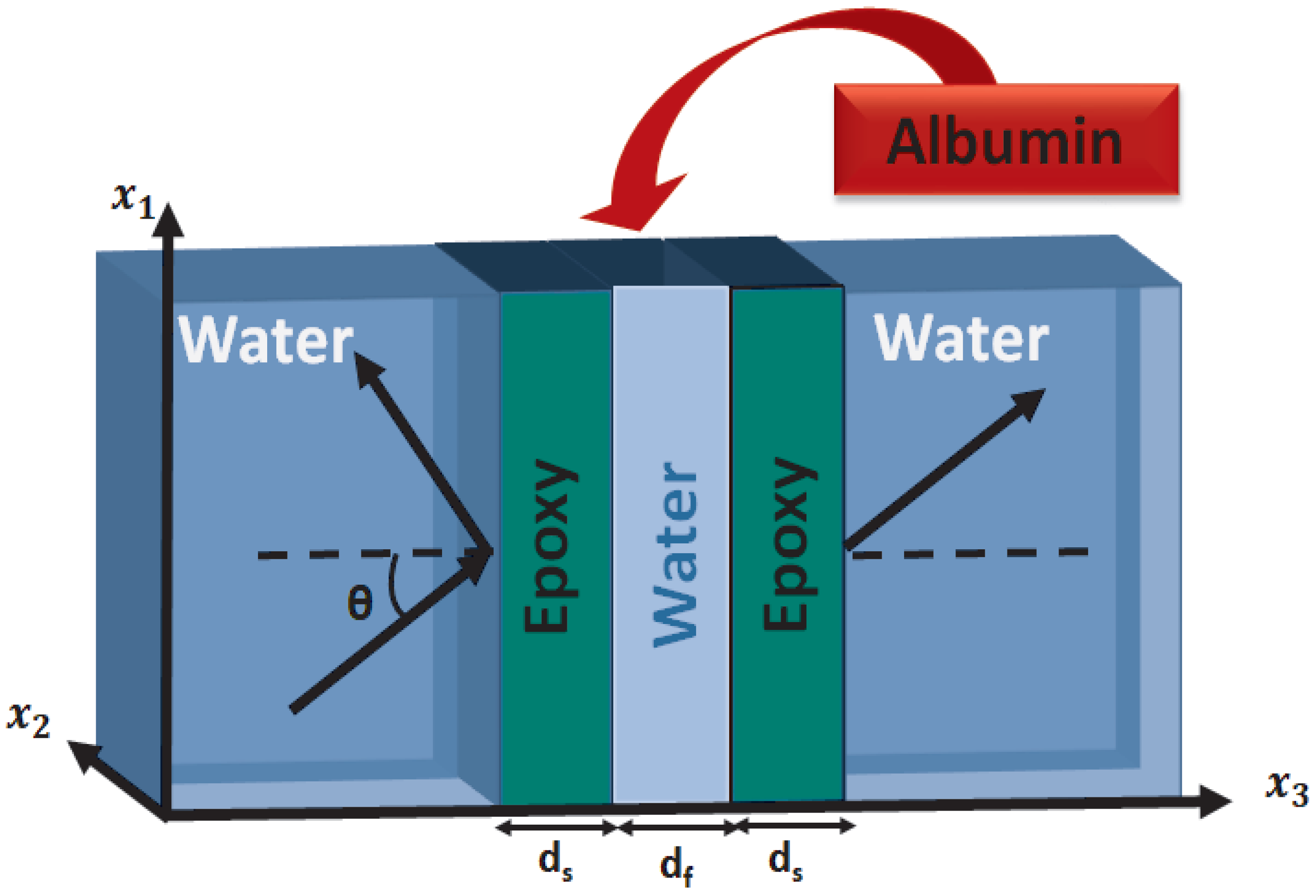
2. Theoretical Model and BIC

2.1. Transmission Coefficient and Dispersion Relation

The calculation method used in this study is based on the interface response theory [42] of continuous media, which allows us to calculate the Green’s function of any composite system. The knowledge of Green’s function enables us to obtain different physical properties of the system, such as the dispersion relations, the transmission and reflection coefficients, as well as the density of states. All the matrix elements $g\left(DD\right)$ in the entire space D of the composite material can be obtained from the knowledge of the matrix elements $g\left(MM\right)$ in the interface space M. $g\left(MM\right)$ is calculated from its inverse $g^{-1}\left(MM\right)$. The latter is formed by a linear superposition of the surface matrix elements $g_i^{-1}(M_i,M_i)$ for each constituent i of the composite system [42].

The system presented in Figure 1 is composed of an epoxy–water–epoxy triple layer immersed in water. The layers are supposed infinite in the $x_1$ and $x_2$ directions. Here, we consider the propagation of acoustic waves polarized in the sagittal plane ($x_1$, $x_3$) defined by the normal to the interfaces ($x_3$ direction) and the wave vector $k_{\mid \mid }$ (parallel to the interfaces). Without a loss of generality, we chose $k_{\mid \mid }$ along the $x_1$ direction. This simplifies considerably the calculation and enables closed form analytical expressions of the dispersion relation of BIC and transmission coefficient. The solid medium (epoxy) is characterized by its thickness $d_s$, longitudinal speed $v_l$, transverse speed $v_t$, and mass density ${\rho }_s$. The liquid layer (sensing layer) is characterized by its thickness $d_f$, velocity $v_f$, and mass density ${\rho }_f$. The surrounding medium (water) is characterized by its velocity $v_0$ and mass density ${\rho }_0$. The inverse Green’s function ${\left[g\left(MM\right)\right]}^{-1}$ of the entire system depicted in Figure 1 in the space of interfaces $M\equiv \{0;d_s;d_s+d_f;2d_s+d_f\}$ is given by [29]

$${\left[g\left(MM\right)\right]}^{-1}=\left(\begin{array}{cccc}{a}_s-F_0& b_s& 0& 0\\ b_s& a_s+a_f& b_f& 0\\ 0& b_f& a_s+a_f& b_s\\ 0& 0& b_s& a_s-F_0\end{array}\right),$$

(1)

where

$$F_0={\rho }_0\frac{{\omega }^2}{{\alpha }_0}\mathrm{and}{\alpha }_0=-j{\left(\frac{{\omega }^2}{v_0^2}-k_{\left|\right|}^2\right)}^{\frac{1}{2}}$$

(2)

characterize the semi-infinite fluid surrounding the triple layer structure,

$$\begin{array}{c}{a}_f=-F\frac{C_f}{S_f},b_f=\frac{F}{S_f},C_f=cosh\left({\alpha }_f{d}_f\right),S_f=sinh\left({\alpha }_f{d}_f\right)\end{array}$$

(3a)

$$\begin{array}{c}F={\rho }_f\frac{{\omega }^2}{{\alpha }_f}\mathrm{and}{\alpha }_f=-j{\left(\frac{{\omega }^2}{v_f^2}-k_{\left|\right|}^2\right)}^{\frac{1}{2}}\end{array}$$

(3b)

characterize the fluid layer, and

$$\begin{array}{c}{a}_s=-\gamma \frac{C_{\ell }}{S_{\ell }}-\beta \frac{C_t}{S_t},b_s=\frac{\gamma }{S_{\ell }}+\frac{\beta }{S_t},\end{array}$$

(4a)

$$\begin{array}{c}\gamma =-\rho \frac{v_t^4}{{\omega }^2{\alpha }_{\ell }}{(k_{\left|\right|}^2+{\alpha }_t^2)}^2,\beta =4\rho \frac{v_t^4}{{\omega }^2}{\alpha }_t{k}_{\left|\right|}^2,\end{array}$$

(4b)

$$\begin{array}{c}{C}_t=cosh\left({\alpha }_t{d}_s\right),C_{\ell }=cosh\left({\alpha }_{\ell }{d}_s\right),S_t=sinh\left({\alpha }_t{d}_s\right),S_{\ell }=sinh\left({\alpha }_{\ell }{d}_s\right),\end{array}$$

(4c)

$$\begin{array}{c}\mathrm{and}{\alpha }_t^2=k_{\left|\right|}^2-\frac{{\omega }^2}{v_t^2},{\alpha }_{\ell }^2=k_{\left|\right|}^2-\frac{{\omega }^2}{v_{\ell }^2}\end{array}$$

(4d)

characterize the two solid layers as similar. $k_{\left|\right|}$ is the component of the wavevector parallel to the layers.

An incident plane wave launched through the structure presented in Figure 1 gives rise to the transmission wave given by [29]

$$t=2F_0\frac{b_f{b}_s^2}{\Delta },$$

(5)

where

$$\Delta =det\left[g^{-1}\left(MM\right)\right]=[(a_s-F)(a_s+a_f-b_f)-b_s^2][(a_s-F)(a_s+a_f+b_f)-b_s^2]$$

(6)

is the determinant of the matrix $g^{-1}\left(MM\right)$ given in Equation (1).

The eigenmodes of the whole system are given by the poles of t (Equation (5)), namely

$$\Delta =0.$$

(7)

In Equation (6), $a_s$, $b_s$, $a_f$, and $b_f$ are real quantities, but $F_0$ can be either real or pure imaginary depending on whether $\omega \le k_{\mid \mid }{v}_0$ or $\omega \ge k_{\mid \mid }{v}_0$, respectively (i.e., below or above the bulk band of the semi-infinite liquid). If $\omega \le k_{\mid \mid }{v}_0$, then $F_0$ (Equation (2)) becomes real, in this case, $\Delta$ (Equation (6)) is real, and its solution gives rise to true eigenmodes. However, if $\omega \ge k_{\mid \mid }{v}_0$, i.e., for frequencies lying inside the continuum modes of the surrounding media, then $\Delta$ (Equation (6)) becomes complex, giving rise to resonant modes (leaky modes) that radiate their energy outside the triple layer. The real part of $\Delta$ gives the position of the resonance, while its imaginary part is related to its width. In general, it is impossible to cancel simultaneously the real and imaginary parts of $\Delta$; however, when this happens, we obtain a BIC. To obtain such BICs, we proceed as follows. First, Equation (5) shows that the transmission zeros are given by

$$b_s=0,$$

(8)

or equivalently,

$$\gamma S_t^{{}^{\prime }}{C}_t^{{}^{\prime }}+\beta S_l^{{}^{\prime }}{C}_l^{{}^{\prime }}=0.$$

(9)

In addition, the eigenmodes of the triple layer with free boundary conditions are given by Equations (6) and (7) by taking $F_0=0$, namely,

$$[a_s(a_s+a_f-b_f)-b_s^2][a_s(a_s+a_f+b_f)-b_s^2]=0$$

(10)

Equation (10) gives two decoupled solutions corresponding to symmetric and asymmetric Lamb modes of the triple layer with free boundary conditions. These modes can be obtained after some algebraic calculation in the following explicit form:

$$\begin{array}{c}2{\alpha }_f{C}_f^{{}^{\prime }}[\gamma C_t^{{}^{\prime }}{S}_l^{{}^{\prime }}+\beta C_l^{{}^{\prime }}{S}_t^{{}^{\prime }}][\gamma S_t^{{}^{\prime }}{C}_l^{{}^{\prime }}+\beta S_l^{{}^{\prime }}{C}_t^{{}^{\prime }}]-{\rho }_f{\omega }^2{S}_f^{{}^{\prime }}[\gamma S_t^{{}^{\prime }}{C}_t^{{}^{\prime }}{C}_l+\beta S_l^{{}^{\prime }}{C}_l^{{}^{\prime }}{C}_t]=0,\end{array}$$

(11a)

$$\begin{array}{c}2{\alpha }_f{S}_f^{{}^{\prime }}[\gamma C_t^{{}^{\prime }}{S}_l^{{}^{\prime }}+\beta C_l^{{}^{\prime }}{S}_t^{{}^{\prime }}][\gamma S_t^{{}^{\prime }}{C}_l^{{}^{\prime }}+\beta S_l^{{}^{\prime }}{C}_t^{{}^{\prime }}]-{\rho }_f{\omega }^2{C}_f^{{}^{\prime }}[\gamma S_t^{{}^{\prime }}{C}_t^{{}^{\prime }}{C}_l+\beta S_l^{{}^{\prime }}{C}_l^{{}^{\prime }}{C}_t]=0,\end{array}$$

(11b)

where $C_f^{{}^{\prime }}=cosh({\alpha }_f{d}_f/2)$ and $S_f^{{}^{\prime }}=sinh({\alpha }_f{d}_f/2)$.

Therefore, if Equations (9) and (11) hold simultaneously, then Equation (10) vanishes, leading to the eigenmodes of the triple layer (i.e., $\Delta =0$) independently of the nature of the surrounding liquids characterized by $F_0$. These modes represent BICs. They are obtained analytically as a consequence of the intersection of the symmetric and antisymmetric Lamb modes of the triple layer (Equations (11a) and (11b)) with the transmission zeros given by Equation (9). In addition, it is worth mentioning that the angle of incidence $\theta$ (Figure 1) is related to the parallel wave vector $k_{\left|\right|}$ by the expression $k_{\left|\right|}=\frac{\omega }{v_0}sin\left(\theta \right)$.

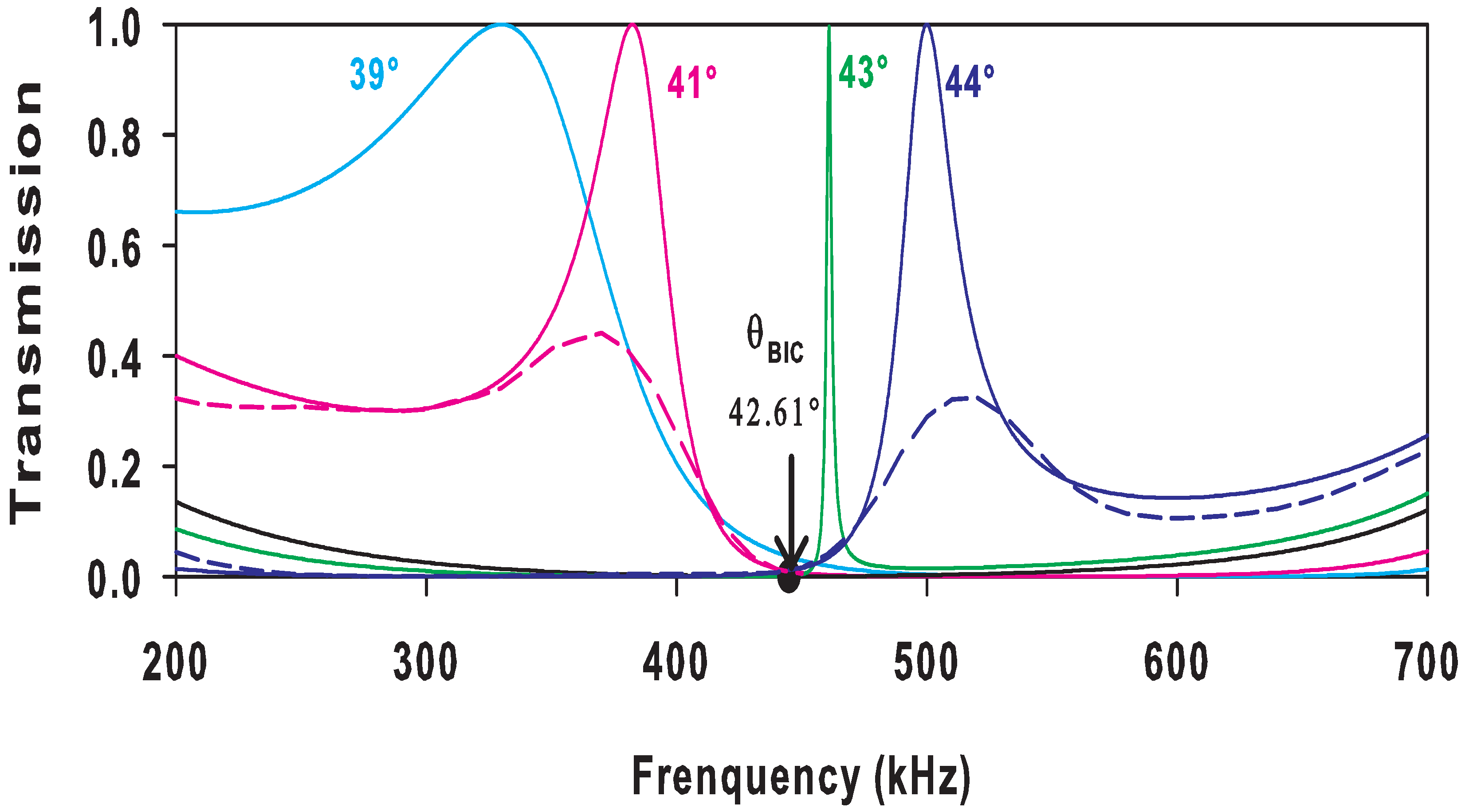
2.2. Example of BIC and Fano Resonance in the Triple Layer

Consider first a solid–liquid–solid triple layer where the two solid layers are made of epoxy and separated by a liquid layer made of water, and the whole structure is immersed in water (Figure 1). The thicknesses of the solid ($d_s$) and liquid ($d_f$) layers are equal ($d_f=d_s=1$ mm), and the materials constants [28] are listed in

Table 1. Velocities of sound and mass densities of epoxy and water.

	$\mathit{\rho }$ (Kg/m${}^3$)	${\mathit{v}}_{\mathit{t}}$ (m/s)	${\mathit{v}}_{\mathit{\ell }}$ (m/s)
Epoxy	1180	1160.8	2539.5
Water	998	-	1486

. Before discussing the usefulness of the intermediate fluid layer as a sensor layer, we shall first recall the existence of the BICs and Fano resonances displayed by the triple layer system where the liquid layer is supposedly made of pure water, identically to the surrounding water media.

Figure 2 shows the transmission coefficients as a function of frequency (kHz) for a perfect phononic structure made of an epoxy–water–epoxy triple layer, where the incident wave is launched from the left (Figure 1) for five angles of incidence: $\theta =39°$, $\theta =41°$, ${\theta }_{BIC}=42.61°$, $\theta =43°$, and $\theta =44°$. The specific angle of incidence ${\theta }_{BIC}=42.61°$ corresponds to the case where the transmission zeros induced by the solid layers and the resonance induced by the triple layers fall at the same frequency of 444.9 kHz. A zero-width resonance occurs, called a BIC, which is characterized by an infinite quality factor Q [29,30]. This mode is indicated by a full circle on the abscissa and is given by Equations (9) and (11). However, when the angle of incidence $\theta$ changes slightly from ${\theta }_{BIC}$, a Fano-type resonance with different shapes appears for $\theta =39°, 41°<{\theta }_{BIC}$ and $\theta =44°, 43°>{\theta }_{BIC}$. In addition, in order to provide information about the transmission spectra in the case of finite size plates, simulations with Comsol Multiphysics software were performed using infinite plane incident waves. The dimensions of the plates are taken as 180 mm × 180 mm × 1 mm as in our recent experiments with water [29]. The numerical results are plotted in Figure 2, with pink and blue dashed lines for $\theta =41°$ and $\theta =44°$, respectively. The shapes of the Fano resonances are quite similar in both analytical and numerical calculations; however, the intensity of the resonances is reduced in the numerical spectra due to the finite size of the plates.

3. A Biosensor Based on BICs and Fano Resonances

The main results represented in this section are divided into three parts: In Section 1, we show how the concentration of albumin affects the transmission spectra and sensor parameters. We take the water resonance frequency as a reference for the resonant peaks position of different concentrations. In Section 2, we study the influence of the angle of incidence on the sensor behavior. In Section 3, we provide the effect of loss on the transmission spectra.

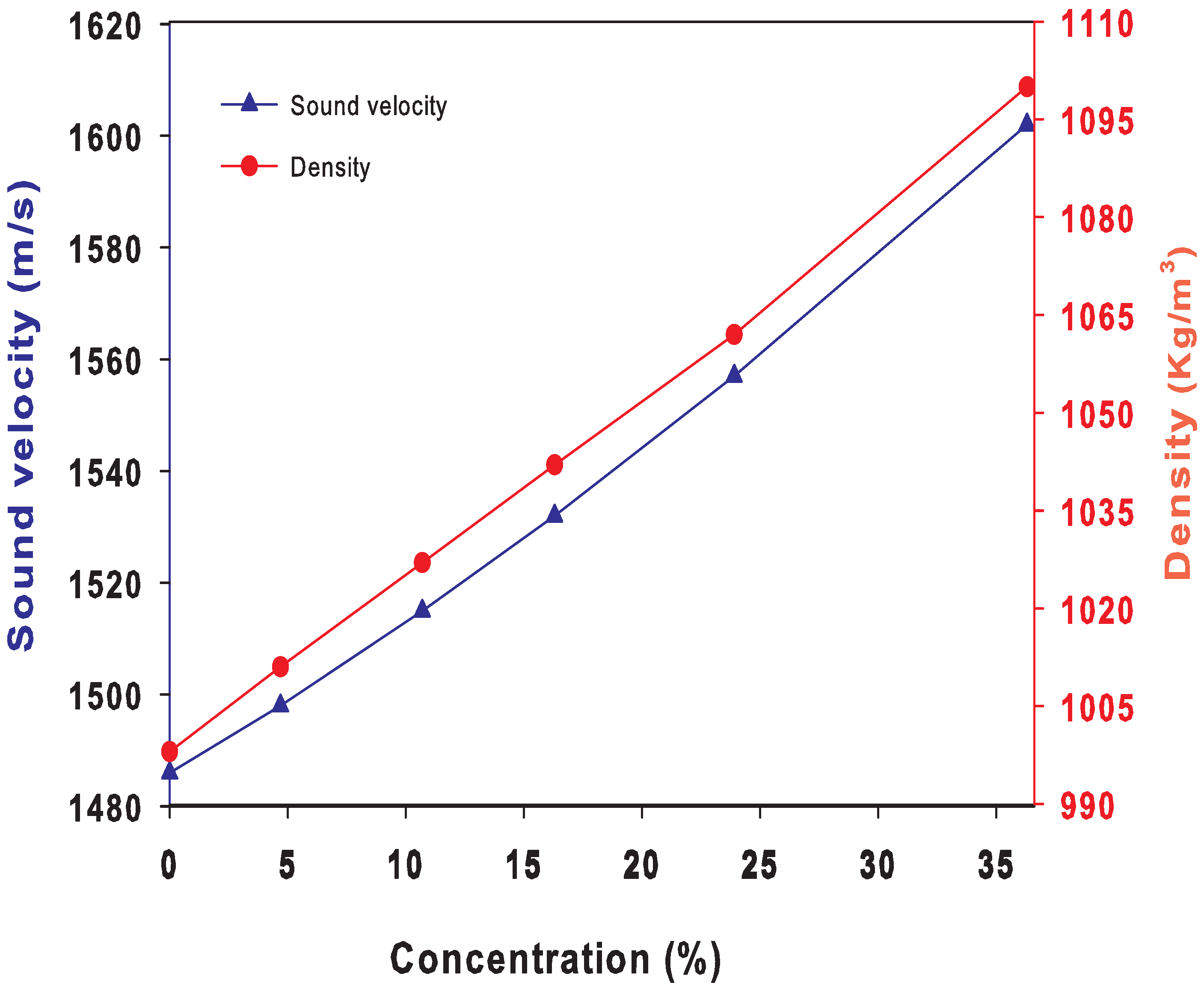
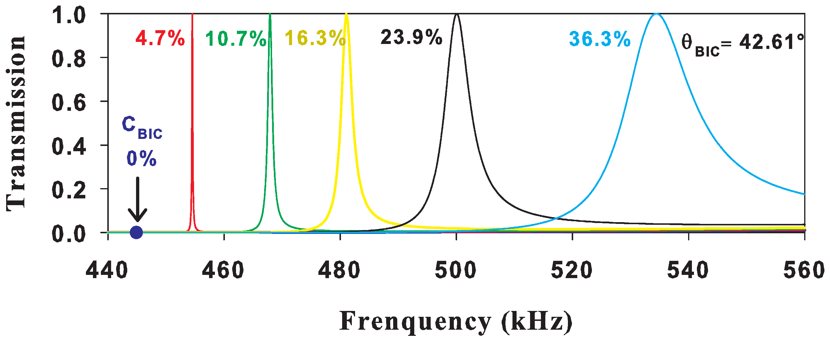
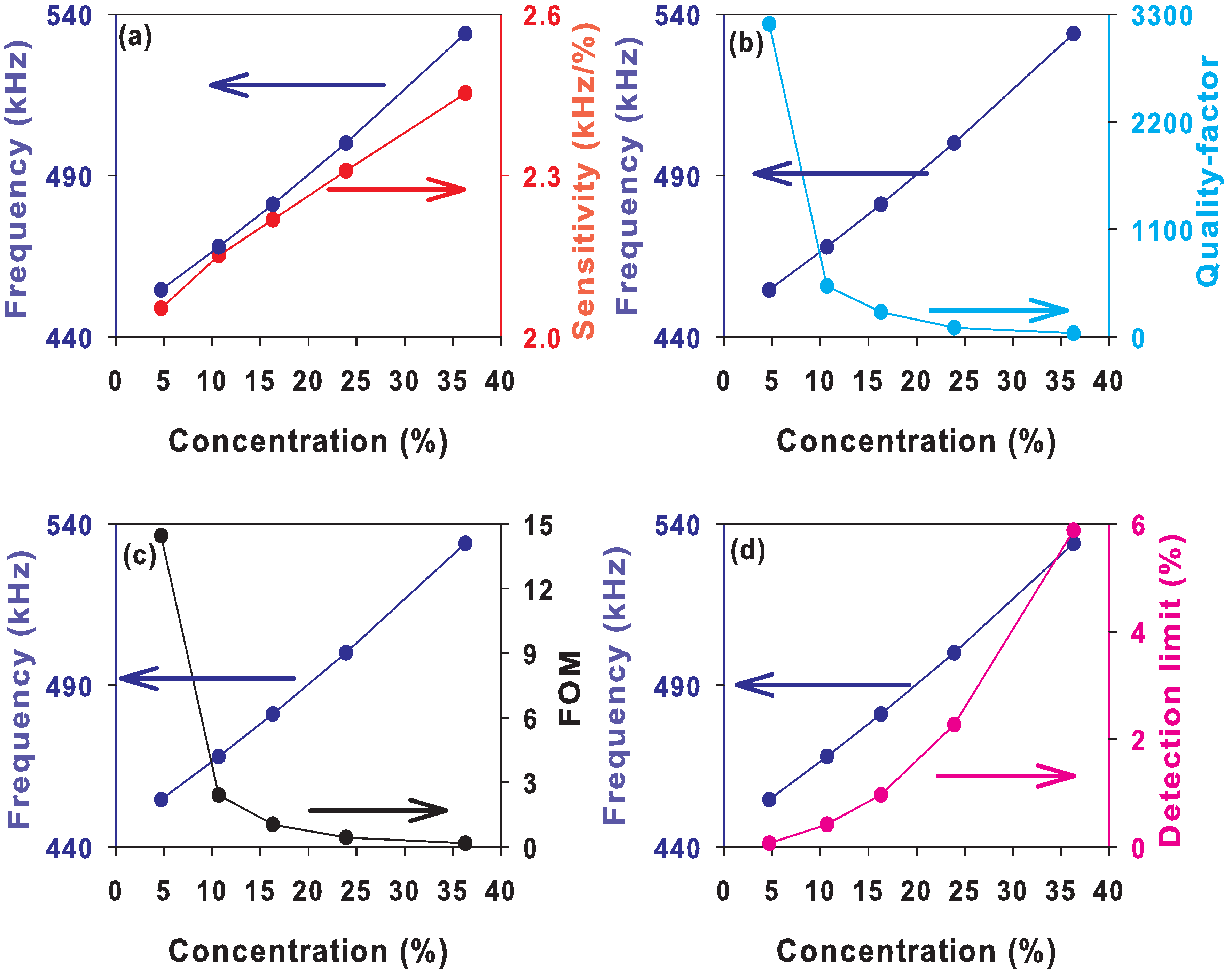
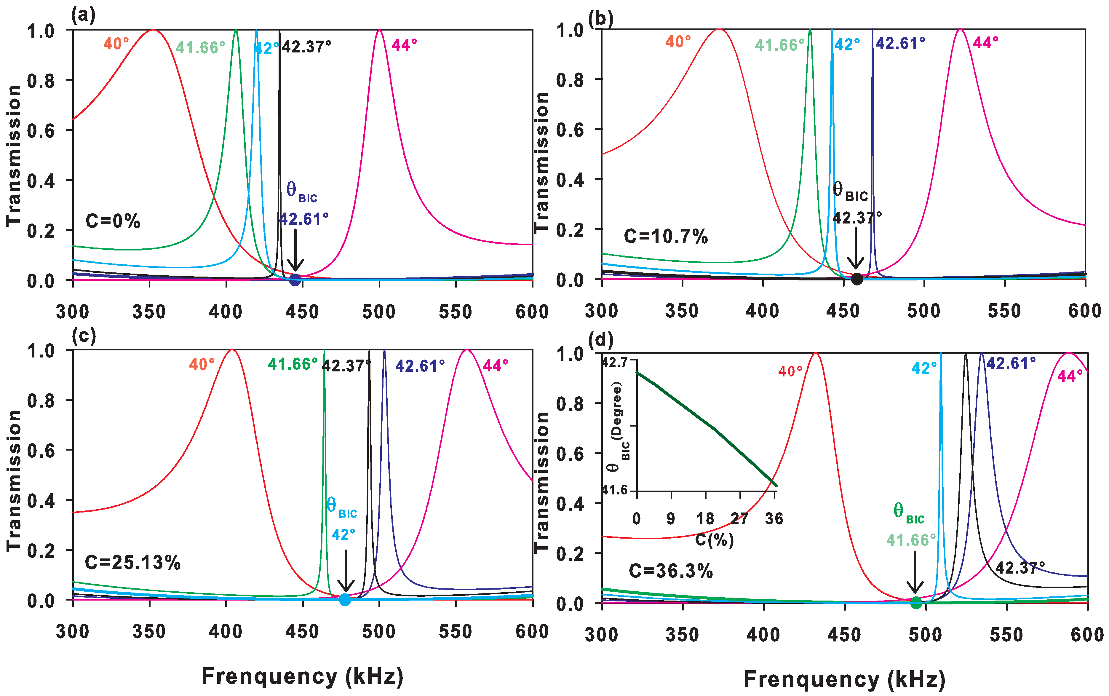
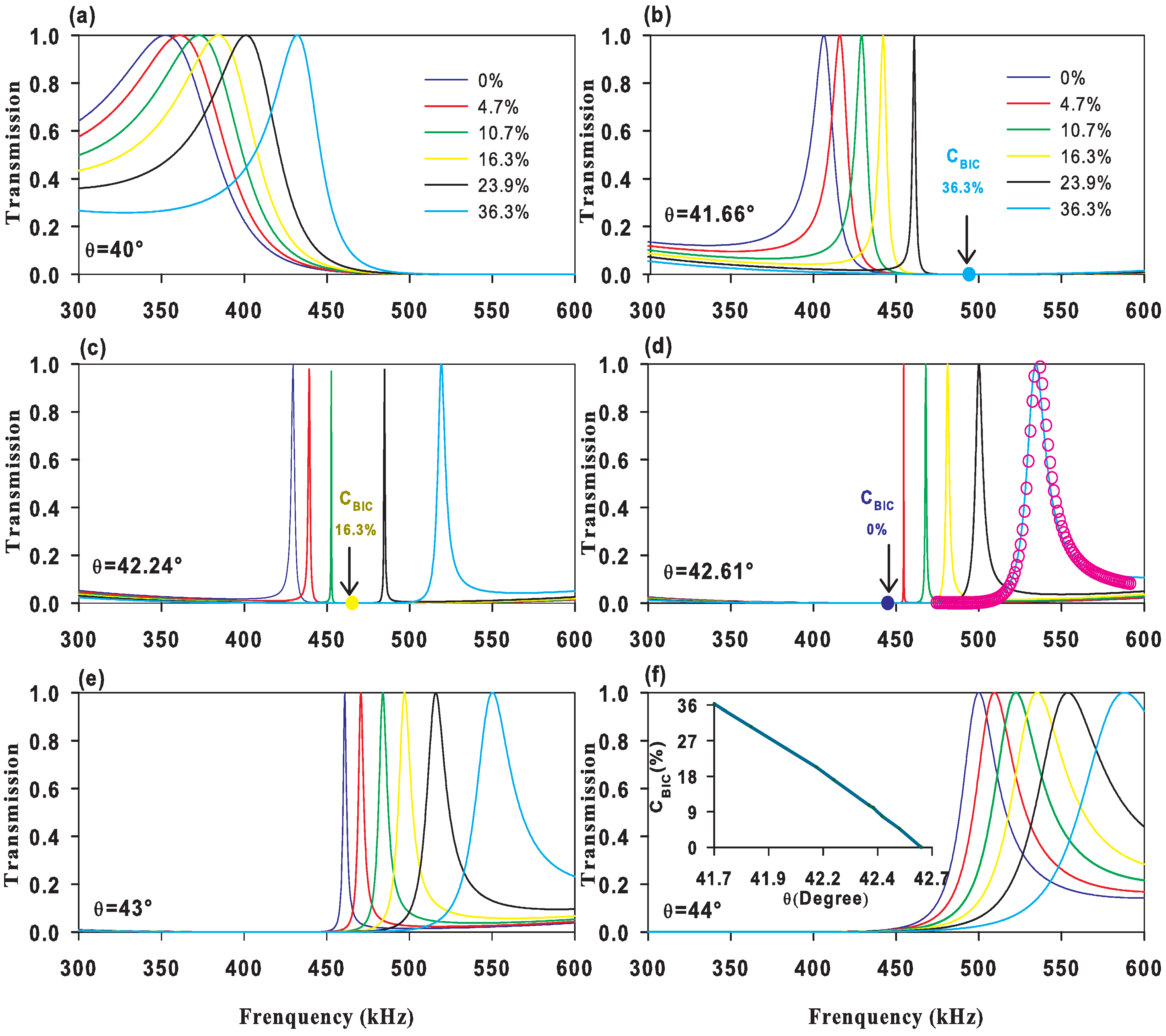
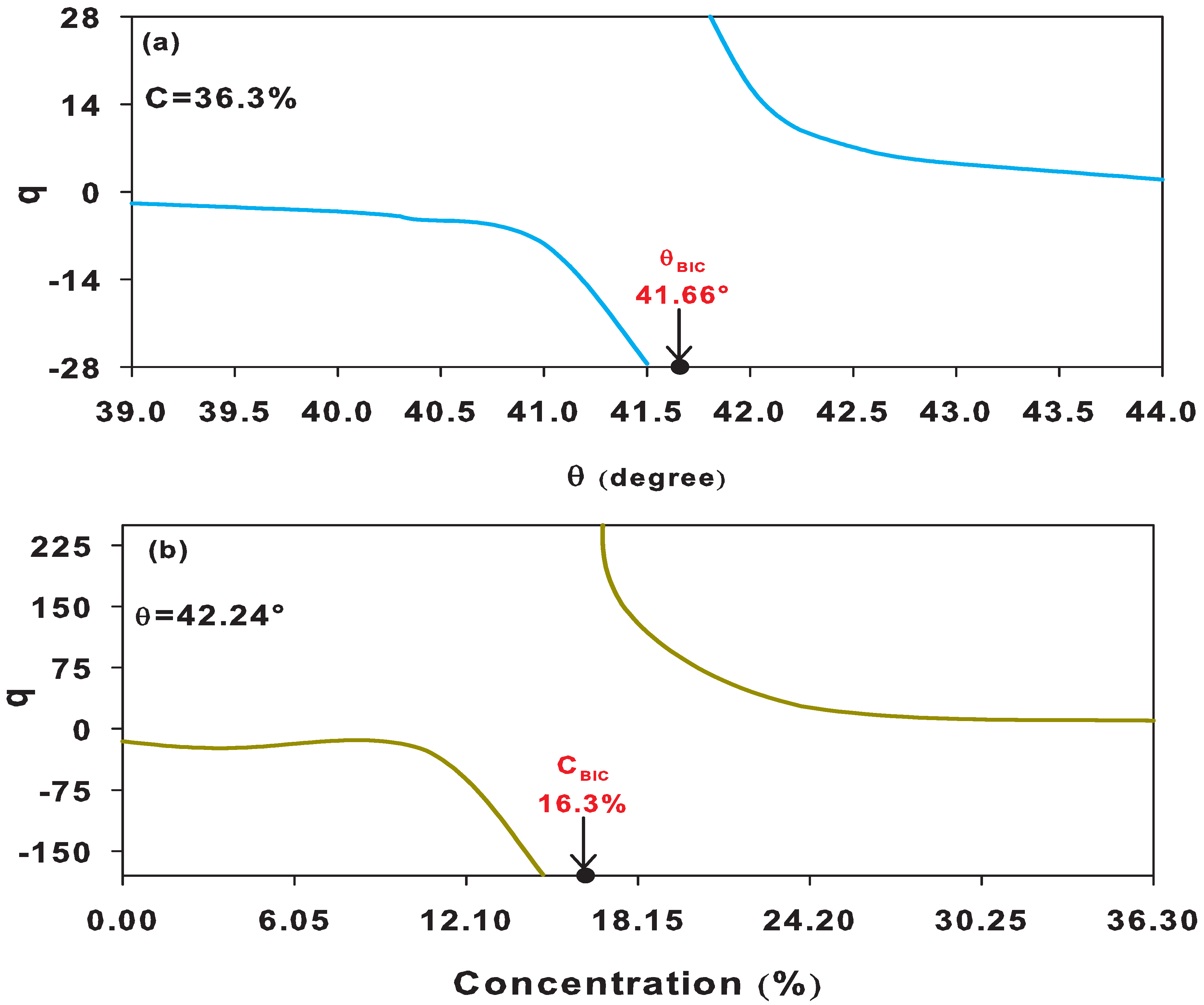
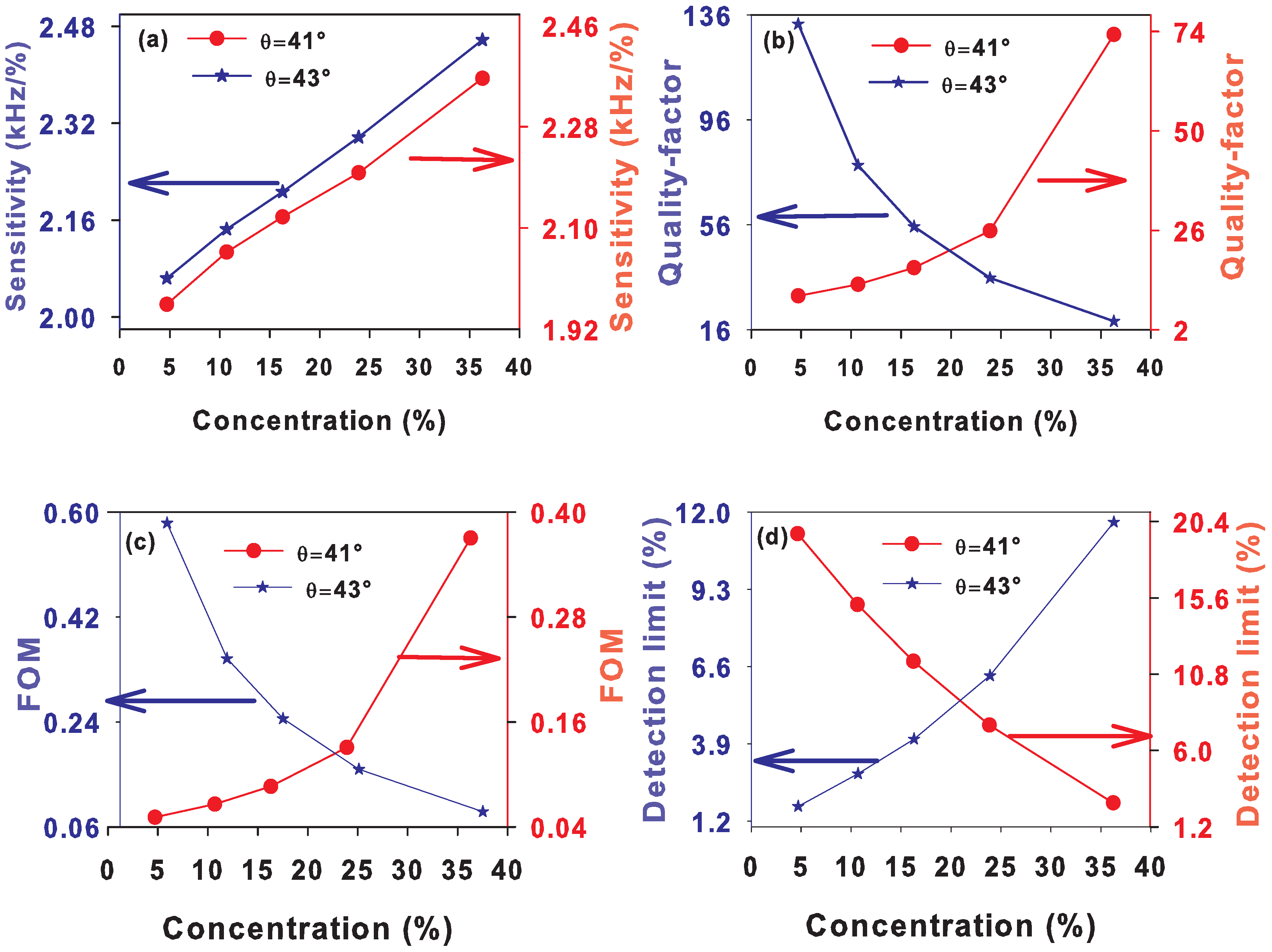
3.1. Effect of the Albumin Concentration

In this subsection, we study the effect of the albumin concentration on the efficiency of the proposed sensor. First, we fixed the angle of incidence at ${\theta }_{BIC}=42.61°$, which corresponds to pure water, and we then exposed the water layer (Figure 1) to different concentrations of albumin between 0 and 36.3% [28,43], so the characteristics of the analyte layer (density and velocity) changed, as shown in Figure 3 [28]. In addition, we extrapolate and determine the acoustic properties for other concentrations of albumin by fitting the curves in Figure 3.

The BIC shown by the vertical arrow in Figure 4 for the water layer ($0\%$ albumin) transforms to a Fano resonance with a maximum of transmission in the vicinity of the transmission zero (indicated by a full circle) induced by the solid layers. As the concentration increases from $0\%$ to $36.3\%$, the width of the Fano resonance increases. The resonance peaks shift to high frequencies from 444.9 to 533.96 kHz. Moreover, since the BIC was chosen for pure water, the system can respond to a small change in the solution concentration of $4.7\%$, in which BICs turns out to transform into a Fano resonance with a high quality factor. Therefore, the performance of the sensor is quite high at small concentrations. It is worth noting that, at an angle of incidence different from ${\theta }_{BIC}$, the results will be different. However, one can obtain a BIC by choosing appropriately the concentration. The performance of the sensor around such a concentration is discussed below.

The performance of a sensor is in general characterized by the sensitivity (S), quality factor (Q), figure of merit (FOM), and detection limit (DL). These parameters [28,44,45,46] are defined by the following expressions:

$$S=\frac{\Delta f}{\Delta C},$$

(12)

$$Q=\frac{f_r}{\Gamma },$$

(13)

$$FOM=\frac{S}{\Gamma },$$

(14)

and

$$DL=\frac{f_r}{Q.S},$$

(15)

where $\Delta f=f_r-f_0$, $f_r$ is the resonance peak for each concentration, and $f_0$ stands for the reference frequency. $\Delta C$ is the concentration change, and $\Gamma$ is the full width at half maximum (FWHM) of the resonance. Note that DL is only the inverse of FOM.

Figure 5a shows that the resonant frequency (blue line) increases with the albumin concentration. Figure 5a shows the sensitivity (red line) versus the concentration for the angle of incidence ${\theta }_{BIC}=42.61°$ and the thickness $d_f$ = $d_s$ = 1 mm. The sensitivity S increases almost linearly when increasing the concentration until it reaches its maximum value S = 2.45 kHz/% at C = 36.3%. Each change in the concentration of about $6\%$ implies a shift of the resonant mode by about 13 kHz, which means that the proposed sensor is characterized by high sensitivity in comparison to a similar structure in the literature [47]. Figure 5b shows the quality factor Q (green line) versus the concentration. Generally, a resonance with a high quality factor means that the resonant peak is very sharp, which improves the frequency resolution. The quality factor reaches the highest value around $Q=3200$ in the vicinity of the BIC. Figure 5c provides the FOM, which is the parameter that predicts the efficiency of the sensor to measure any change in resonant frequency. Its maximum value is FOM = 14.45. The maximum range of both Q and FOM are located in the vicinity of the BIC frequency at only $4.7\%$ albumin. Q and FOM decrease as the concentration increases and tend towards limiting values, namely, Q = 37 and FOM = 0.17 for high concentrations when the Fano resonance deviates from the BIC.

Figure 5d represents the DL versus the albumin concentration. This quantity is known as the minimum amount of analyte concentration that can be accurately detected. Indeed, DL is defined as the inverse of FOM, so the best (i.e., lowest) DL that the sensor can accurately detect is DL = 0.069% for the concentration C = 4.7% at the angle of incidence ${\theta }_{BIC}=42.61°$.

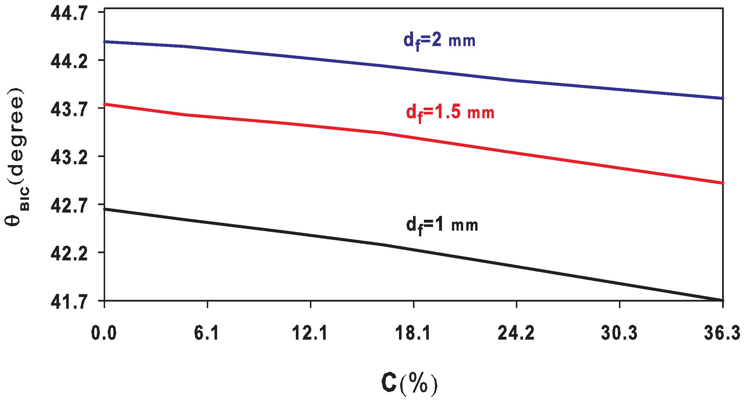
3.2. Effect of the Angle of Incidence

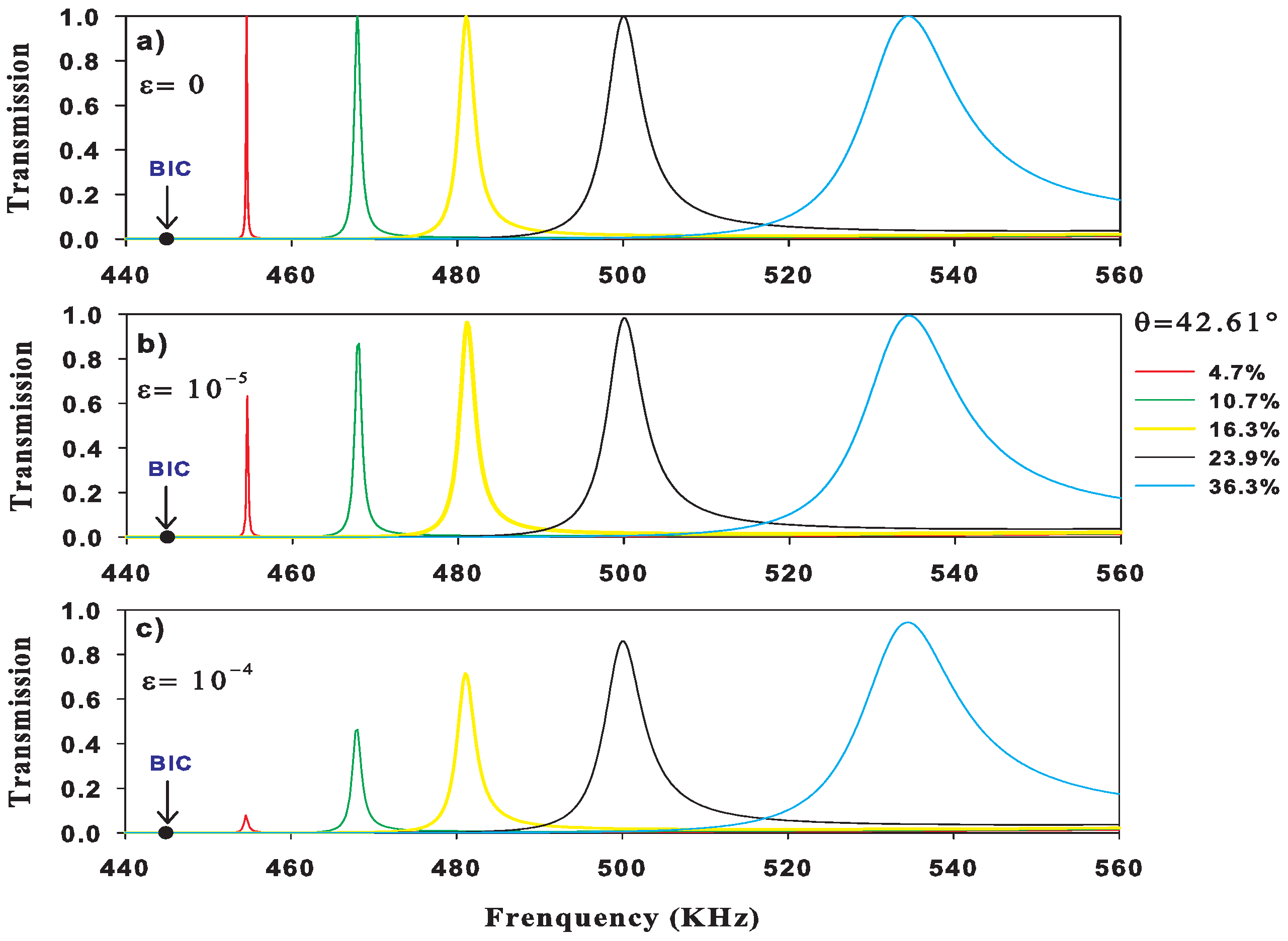
For a better overview of the effect of the angle of incidence on the sensor efficiency, we fixed the layer thicknesses at $d_s=d_f$ = 1 mm, and for different concentrations, C = 0% (Figure 6a), C = 10.7% (Figure 6b), C = 25.13% (Figure 6c), and C = 36.3% (Figure 6d), we plotted the transmission coefficients for different values of the angle of incidence, as shown in Figure 6. The resonance peaks shift to high frequencies as the angle of incidence increases for each concentration. For each concentration, there is an angle of incidence corresponding to a BIC (${\theta }_{BIC}$). Around the ${\theta }_{BIC}$, the BIC transforms to a Fano resonance with an opposite asymmetric Fano shape (see below). When C increases from 0 to 36.3%, the Fano resonances move to the right-hand side of the BIC. The evolution of the ${\theta }_{BIC}$ as a function of the concentration C is given in the inset of Figure 6d, which shows a decrease in ${\theta }_{BIC}$ versus C.

Figure 7 shows the transmission spectra of the structure as a function of frequency for different albumin concentrations in the range 0–36.3% and for different angles of incidence: $\theta =40°$ (Figure 7a), $\theta =41.66°$ (Figure 7b), $\theta =42.24°$ (Figure 7c), $\theta =42.61°$ (Figure 7d), $\theta =43°$ (Figure 7e), and $\theta =44°$ (Figure 7f). Similarly to Figure 6, one can see that, for each angle of incidence, there is a concentration corresponding to a BIC ($C_{BIC}$). Around the $C_{BIC}$, the BIC transforms to a Fano resonance with an opposite asymmetric Fano shape (see below). When $\theta$ increases from $40°$ to $44°$, the asymmetric line shape of the Fano resonance changes around the BIC. The variation of the $C_{BIC}$ as a function of the angle of incidence $\theta$ is given in the inset of Figure 7f. The concentration $C_{BIC}$ manifests a decrease versus the angle of incidence $\theta$. These results show that, for the sensor to achieve a good performance around a given concentration, we an appropriate angle of incidence must be chosen. It is worth noticing that, in our recent experimental paper [30], the precision angle setting is given with a decimal point. We have checked that the transmission spectra in general and the BIC in particular remain robust when the angles of incidence are taken with one decimal point instead of two.

In order to ensure that the resonances presented above are of Fano type, we show in Figure 7d the fitted results (open circles) for $\theta =42.61°$ and $C=36.3\%$ based on the Fano formula:

$$T=A\frac{{(\omega -{\omega }_R+q\Gamma )}^2}{{(\omega -{\omega }_R)}^2+{\Gamma }^2},$$

(16)

where $A=\frac{1}{q^2}$, ${\omega }_R$, and $\Gamma$ are the standard parameters that denote the position and the width of the resonance, respectively. q is the so-called Fano parameter that describes the degree of asymmetry of the resonance. Figure 7d gives a comparison between the exact results of the transmission coefficient (solid cyan curve) and the curve obtained from Equation (16) (open circles) for $\theta =42.61°$ and $C=36.3\%$. A good fit is obtained with the following parameters $q=6.193$ and $\Gamma =14.45$ kHz.

In Figure 5, we show that the best sensitivity is obtained for a high concentration C of 36.3%. In Figure 8, we show a comparison of the sensor parameters as a function of the angle of incidence where the concentration C = 36.3% and thicknesses $d_f$ and $d_s$ = 1 mm. The sensitivity shown in Figure 8a reaches its maximum value S = 2.47 kHz/% for the angle of incidence $\theta =42.24°$ close to the BIC. Moreover, the Q factor and FOM in Figure 8b,c, respectively, reach their maximum values when the angle of incidence $\theta$ approaches the one corresponding to the BIC and tend towards infinity around ${\theta }_{BIC}=41.66°$. The best detection limit close to zero ($DL=0.0153\%$) is obtained around ${\theta }_{BIC}$ (Figure 8d).

Figure 9a shows the behavior of the Fano parameter as a function of $\theta$ for $C=36.3\%$. One can see that q diverges at ${\theta }_{BIC}=41.66°$ and takes opposite values for $\theta$ on both sides of ${\theta }_{BIC}$. Similar results are obtained for the variation of q versus the concentration for $\theta =42.24°$ (Figure 9b). Here, q diverges at $C_{BIC}=16.3\%$ and takes opposite values around $C_{BIC}$.

In Figure 9a, we show the variation of the sign of the Fano parameter q around ${\theta }_{BIC}$, which is related to the asymmetry of the Fano resonance. The sensor parameters versus the concentration depend considerably on whether the q parameter is positive or negative. Figure 10 compares the sensor parameters for $\theta =41°$ (q = −8.28) and $\theta =43°$ (q = 4.48). The thicknesses of the layers are set at $d_s$ and $d_f$ = 1 mm. Figure 10a shows the sensitivity of the albumin sensor versus the concentration for $\theta =41°$ (red circles) and $\theta =43°$ (blue stars). It appears that the sensitivity of the sensor increases with the concentration for both incidence angles, with an improved sensitivity for the angle of incidence $\theta =43°$. On the other hand, the quality factor presented in Figure 10b increases with the concentration for the angle of incidence $\theta =41°$ until it reaches its maximum value at $C=36.3\%$, which is due to the fact that the width of the Fano resonance shrinks at $C=36.3\%$ and collapses close to the BIC, whereas for the angle $\theta =43°$, the quality factor decreases versus the concentration and becomes maximum at the concentration $C=4.7\%$ in the vicinity of the BIC. Similar behavior occurs for the FOM (Figure 10c) as both quantities (Q and FOM) are inversely proportional to the width of the resonance (Equations (13) and (14)). It also appears from Equation (15) that a higher quality factor obtains a lower detection limit. Thus, the minimum detection limit of the proposed sensor for both angles $\theta =41°$ and $\theta =43°$ appears at the concentrations $C=36.3\%$ and $C=4.7\%$, respectively, as shown in Figure 10d.

The above results are presented for fixed thicknesses of the liquid and solid layers ($d_s=d_f=1$ mm). If both thicknesses are changed by a scale factor $\alpha$, then all results remain the same with a scale of the frequencies by a factor $1/\alpha$. For other choices of thicknesses, the physical conclusions hold, but quantitatively, the ${\theta }_{BIC}$ associated with each concentration will change to a new value. This enables experiments on samples with $d_f$ other than the considered value of 1 mm by taking an appropriate incidence angle. Figure 11 shows the variation of the concentration as a function of the angle of incidence ${\theta }_{BIC}$ for three values of the thickness of the sensing liquid layer. One can see that, for each concentration, there is an angle ${\theta }_{BIC}$ that depends on the thickness of the sensing layer.

We provide in

Table 2. A comparison between the design Q factor of our sensor with those of previous sensors.

Types of Device	Q-Factor	Reference
1D phononic crystal from lead and epoxy with defect layer from glycine	Ranges from 8502 to 13497	Khateib et al. [48]
1D phononic crystal from lead and water with defect layer from glucose or H${}_2$O${}_2$	5196	Mehaney et al. [49]
Slotted phononic crystal composed of Silicon	6095	Geng et al. [50]
2D periodic structure made of identical cylindrical holes in presence of a liquid-filled cylindrical cavity defect	1000	Mukhin et al. [51]
Solid–liquid–solid triple layer sensor	Ranges from 3201 to infinity	Present work

a comparison between the quality factor of the proposed sensor and those of sensors published in the literature. It is obvious that the structure presented in this work presents high quality factors that tend towards infinity at the BIC. The sensitivity obtained in this work around S = 2.47 kHz/% is higher than that obtained with a millimetric structure operating in a few hundred kHz by Lucklum et al. [47] (1.4 kHz/%).

3.3. Effect of Loss

In the above results, the materials were considered lossless. However, the shape of Fano resonances could be considerably affected when loss is taken into account, especially in the vicinity of the BIC. We consider here the effect of absorption on Fano resonance discussed in Section 3.1. The dissipation can be included by adding a small imaginary part to the transverse and longitudinal velocities of sound in solid layers such that $C_t^{\prime }=C_t(1+jϵ)$ and $C_l^{\prime }=C_t(1+jϵ)$ [52,53].

Figure 12 shows the transmission coefficient as a function of the frequency for different concentrations at the angle of incidence $\theta =42.61°$ and for the thicknesses of the layers such that $d_f$ and $d_s$ = 1 mm. In this figure, the epoxy layer is considered without loss (Figure 12a), with small loss $ϵ={10}^{-5}$ (Figure 12b), and with high loss $ϵ={10}^{-4}$ (Figure 12c). As absorption increases, the intensity of Fano resonances decreases, especially when the resonance approaches the BIC frequency for small concentrations. For high concentrations, the Fano resonances are less sensitive to the effect of loss and remain almost unchanged because the resonances are broader (with smaller quality factors). These results show that, if solid layers with less loss are used, then even the transmission peaks near the BIC can be observed.

4. Conclusions

We propose a simple acoustic multilayer to design an efficient biosensor that can detect different concentrations of albumin. The proposed structure made of an epoxy–albumin–epoxy triple layer immersed in water allowed us to induce a resonance with zero width, the so-called BIC at $0\%$ albumin (i.e., pure water) for a particular angle of incidence ${\theta }_{BIC}=42.61°$ and layer thicknesses $d_s=d_f=1$ mm. By supplementing an admixture of albumin to the water layer, BICs can be transformed into Fano resonances characterized by high quality factors that are very sensitive to the concentration of albumin. We found an efficient response of the sensor to a small albumin concentration ($4.7\%$) with a high quality factor, a high figure of merit, and a minimum detection limit, without perturbing the geometry of the structure. The importance of the detection limit lies in the ability of a sensor to detect a low concentration value. Afterward, we studied the sensor behavior when changing the angle of incidence. The best performance of the sensor was found around the structure parameters that give rise to the BIC. Finally, we considered the effect of loss on the shape of the Fano resonance. The intensity of the resonance in the vicinity of the BIC changes drastically for small concentrations, while it remains stable as the concentration increases. The investigation of the transmission coefficient, sensitivity, and sensor parameters was performed by means of Green’s function method. The experimental validation of these theoretical results is in progress.

In addition to Table 2, where we highlight some advantages of the proposed platform over other types of biosensor, there are other virtues of such a sensor worth mentioning:

(i) The simplicity of the structure consists of sandwiching a liquid sensor layer between two solid layers. The solid layers induce transmission zeros that enable one to obtain a large transmission gap, while the sensor layer enables one to introduce a Fano resonance with a high sensitivity and low detection limit.

(ii) The simplicity of the analytical calculation helps in indicating the appropriate angle of incidence required to obtain BICs and Fano resonances.

(iii) It is possible to use the proposed triple layer sensor in other application contexts, such as water pollution (contamination with biological and chemical particles) as well as other fluids such harmful gases for health.

(iv) We can use a multilayered structure with two or more sensor layers separated by solid layers, and each liquid layer can then detect a selected admixture through an analysis of its own Fano resonance.

References

1. Lucklum, R.; Li, J. Phononic crystals for liquid sensor applications. Meas. Sci. Technol. 2009, 20, 124014. [Google Scholar] [CrossRef]
2. Amoudache, S.; Pennec, Y.; Djafari-Rouhani, B.; Khater, A.; Lucklum, R.; Tigrine, R. Simultaneous sensing of light and sound velocities of fluids in a two-dimensional phoXonic crystal with defects sensing. J. Appl. Phys. 2014, 115, 134503. [Google Scholar] [CrossRef]
3. Khansili, N.; Rattu, G.; Krishna, P.M. Label-free optical biosensors for food and biological sensor applications. Sens. Actuators B Chem. 2018, 265, 35–49. [Google Scholar] [CrossRef]
4. Theint, H.T.; Walsh, J.E.; Wong, S.T.; Von, K.; Shitan, M. Development of an optical biosensor for the detection of Trypanosoma evansi and Plasmodium berghei. Spectrochim. Acta A 2019, 2018, 348–358. [Google Scholar] [CrossRef] [PubMed]
5. Loyez, M.; Larrieu, J.C.; Chevineau, S.; Remmelink, M.; Leduc, D.; Bondue, B.; Lambert, P.; Devière, J.; Wattiez, R.; Caucheteur, C. In situ cancer diagnosis through online plasmonics. Biosens. Bioelectron. 2019, 131, 104–112. [Google Scholar] [CrossRef] [Green Version]
6. Casadio, S.; Lowdon, J.W.; Betlem, K.; Ueta, J.T.; Foster, C.W.; Cleij, T.J.; van Grinsven, B.; Sutcliffe, O.B.; Banks, C.E.; Peeters, M. Development of a novel flexible polymer-based biosensor platform for the thermal detection of noradrenaline in aqueous solutions. Chem. Eng. J. 2017, 315, 459–468. [Google Scholar] [CrossRef]
7. Wang, Z.; Jinlong, L.; An, Z.; Kimura, M.; Ono, T. Enzyme immobilization in completely packaged freestanding SU-8 microfluidic channel by electro click chemistry for compact thermal biosensor. Process Biochem. 2019, 79, 57–64. [Google Scholar] [CrossRef]
8. Khan, M.S.; Misra, S.K.; Dighe, K.; Wang, Z.; Schwartz-Duval, A.S.; Sar, D.; Pan, D. Electrically-receptive and thermally-responsive paper-based sensor chip for rapid detection of bacterial cells. Biosens. Bioelectron. 2018, 110, 132–140. [Google Scholar] [CrossRef] [Green Version]
9. Zaremanesh, M.; Carpentier, L.; Gharibi, H.; Bahrami, A.; Mehaney, A.; Gueddida, A.; Lucklum, R.; Djafari-Rouhani, B.; Pennec, Y. Temperature biosensor based on triangular lattice phononic crystals. APL Mater. 2021, 9, 061114. [Google Scholar] [CrossRef]
10. Jenik, M.; Schirhagl, R.; Schirk, C.; Hayden, O.; Lieberzeit, P.; Blaas, D.; Paul, G.; Dickert, F.L. Sensing picornaviruses using molecular imprinting techniques on a quartz crystal microbalance. Anal. Chem. 2009, 81, 5320–5326. [Google Scholar] [CrossRef]
11. Schirhagl, R.; Lieberzeit, P.A.; Dickert, F.L. Chemosensors for viruses based on artificial immunoglobulin copies. Adv. Mater. 2010, 22, 2078–2081. [Google Scholar] [CrossRef] [PubMed]
12. Zhang, Z.; Sohgawa, M.; Yamashita, K.; Noda, M. A micromechanical cantilever-based liposome biosensor for characterization of protein-membrane interaction. Electroanalysis 2016, 28, 620–625. [Google Scholar] [CrossRef]
13. Tardivo, M.; To oli, V.; Fracasso, G.; Borin, D.; Dal Zilio, S.; Colusso, A.; Carrato, S.; Scoles, G.; Meneghettie, M.; Colombatti, M.; et al. Parallel optical read-out of micromechanical pillars applied to prostate specific membrane antigen detection. Biosens. Bioelectron. 2015, 72, 393–399. [Google Scholar] [CrossRef] [PubMed]
14. Voiculescu, I.; Nordin, A.N. Acoustic wave based MEMS devices for biosensing applications. Biosens. Bioelectron. 2012, 33, 1–9. [Google Scholar] [CrossRef] [PubMed]
15. Fan, X.; White, I.M.; Shopova, S.I.; Zhu, H.; Suter, J.D.; Sun, Y. Sensitive optical biosensors for unlabeled targets: A review. Anal. Chim. Acta 2008, 620, 8–26. [Google Scholar] [CrossRef] [PubMed]
16. Oh, S.Y.; Heo, N.S.; Shukla, S.; Cho, H.J.; Vilian, A.T.E.; Kim, J.; Lee, S.Y.; Yoo, S.M.; Huh, Y.S. Development of gold nanoparticle-aptamer-based LSPR sensing chips for the rapid detection of Salmonella typhimurium in pork meat. Sci. Rep. 2017, 7, 10130. [Google Scholar] [CrossRef] [PubMed] [Green Version]
17. Ji, J.; Pang, Y.; Li, D.; Huang, Z.; Zhang, Z.; Xue, N.; Xui, Y.; Mu, X. An aptamer-based shear horizontal surface acoustic wave biosensor with a CVD-grown single-layered graphene film for high-sensitivity detection of a label-free endotoxin. Microsyst. Nanoeng. 2020, 6, 4. [Google Scholar] [CrossRef] [Green Version]
18. Lec, R.M.; Lewin, P.A. Acoustic wave biosensors. In Proceedings of the Proceedings of the 20th Annual International Conference of the IEEE Engineering in Medicine and Biology Society. Vol. 20 Biomedical Engineering Towards the Year 2000 and Beyond (Cat. No.98CH36286), Hong Kong, China, 1 November 1998; Volume 6, pp. 2779–2784. [Google Scholar]
19. Drafts, B. Acoustic wave technology sensors. IEEE Trans. Microw. Theory Tech. 2001, 49, 795–802. [Google Scholar] [CrossRef]
20. Liang, C.; Peng, H.; Nie, L.; Yao, S. Bulk acoustic wave sensor for herbicide assay based on molecularly imprinted polymer. Fresen. J. Anal. Chem. 2000, 367, 551–555. [Google Scholar] [CrossRef]
21. Peng, H.; Liang, C.; Zhou, A.; Zhang, Y.; Xie, Q.; Yao, S. Development of a new atropine sulfate bulk acoustic wave sensor based on a molecularly imprinted electro synthesized copolymer of aniline with o-phenylenediamine. Anal. Chim. Acta 2000, 423, 221–228. [Google Scholar] [CrossRef]
22. Gronewold, T.M. Surface acoustic wave sensors in the bioanalytical field: Recent trends and challenges. Anal. Chim. Acta 2007, 603, 119–128. [Google Scholar] [CrossRef] [PubMed]
23. Arsat, R.; Breedon, M.; Shafiei, M.; Spizziri, P.G.; Gilje, S.; Kaner, R.B.; Kalantar-zadeh, K.; Wlodarski, W. Graphene-like nano-sheets for surface acoustic wave gas sensor applications. Chem. Phys. Lett. 2009, 467, 344–347. [Google Scholar] [CrossRef]
24. Oseev, A.; Lucklum, R.; Zubtsov, M. Gasoline properties determination with phononic crystal cavity sensor. Sens. Actuators B 2013, 189, 208. [Google Scholar] [CrossRef]
25. Zubtsov, M.; Lucklum, R.; Ke, M.; Oseev, A.; Grundmann, R.; Henning, B.; Hempel, U. 2D phononic crystal sensor with normal incidence of sound. Sens. Actuators A 2012, 186, 118. [Google Scholar] [CrossRef]
26. Mukhin, N.; Kutia, M.; Oseev, A.; Steinmann, U.; Palis, S.; Lucklum, R. Narrow band solid–liquid composite arrangements: Alternative solutions for phononic crystal-based liquid sensors. Sensors 2019, 19, 3743. [Google Scholar] [CrossRef] [Green Version]
27. Villa-Arango, S.; Torres, R.; Kyriacou, P.A.; Lucklum, R. Fully-disposable multilayered phononic crystal liquid sensor with symmetry reduction and a resonant cavity. Measurement 2017, 102, 20–25. [Google Scholar] [CrossRef]
28. Khateib, F.; Mehaney, A.; Amin, R.M.; Aly, A.H. Ultra-sensitive acoustic biosensor based on a 1D phononic crystal. Phys. Scr. 2020, 95, 075704. [Google Scholar] [CrossRef]
29. Quotane, I.; El Boudouti, E.H.; Djafari-Rouhani, B. Trapped-mode-induced Fano resonance and acoustical transparency in a one-dimensional solid-fluid phononic crystal. Phys. Rev. B 2018, 97, 024304. [Google Scholar] [CrossRef]
30. Amrani, M.; Quotane, I.; Ghouila-Houri, C.; Krutyansky, L.; Piwakowski, B.; Pernod, P.; Talbi, A.; Djafari-Rouhani, B. Experimental Evidence of the Existence of Bound States in the Continuum and Fano Resonances in Solid–liquid Layered Media. Phys. Rev. Appl. 2021, 15, 054046. [Google Scholar] [CrossRef]
31. Hsu, C.W.; Zhen, B.; Stone, A.D.; Joannopoulos, J.D.; Soljacic, M. Bound states in the continuum. Nat. Rev. Mater. 2016, 1, 16048. [Google Scholar] [CrossRef] [Green Version]
32. Von Neuman, J.; Wigner, E. On some peculiar discrete eigenvalues. Phys. Z. 1929, 30, 465. [Google Scholar]
33. Gaidarzhy, A.; Imboden, M.; Rankin, J.; Sheldon, B.W. High quality factor gigahertz frequencies in nanomechanical diamond resonators. Appl. Phys. Lett. 2007, 91, 203503. [Google Scholar] [CrossRef] [Green Version]
34. Romano, S.; Zito, G.; Torino, S.; Calafiore, G.; Penzo, E.; Coppola, G.; Cabrini, S.; Rendina, I.; Mocella, V. Label-free sensing of ultralow-weight molecules with all-dielectric metasurfaces supporting bound states in the continuum. Photonics Res. 2018, 6, 7. [Google Scholar] [CrossRef]
35. Romano, S.; Mangini, M.; Cabrini, S.; De Luca, A.C.; Rendina, I.; Mocella, V.; Zito, G. Ultrasensitive Surface Refractive Index Imaging Based on Quasi-Bound States in the Continuum. ACS Nano 2020, 14, 15417–15427. [Google Scholar] [CrossRef]
36. Wang, S.; Cheng, Q.; LV, J.; Wang, J. Photonic crystal sensor based on Fano resonances for simultaneous detection of refractive index and temperature. J. Appl. Phys. 2020, 128, 034501. [Google Scholar] [CrossRef]
37. Ahmadivand, A.; Gerislioglu, B. Photonic and Plasmonic Metasensors. Laser Photonics Rev. 2021, 16, 2100328. [Google Scholar] [CrossRef]
38. Gerislioglu, B.; Dong, L.; Ahmadivand, A.; Hu, H.; Nordlander, P.; Halas, N.J. Monolithic metal dimer-on-film structure: New plasmonic properties introduced by the underlying metal. Nano Lett. 2020, 20, 2087–2093. [Google Scholar] [CrossRef]
39. Alipour, A.; Farmani, A.; Mir, A. High Sensitivity and Tunable Nanoscale Sensor Based on Plasmon-Induced Transparency in Plasmonic Metasurface. IEEE Sens. J. 2018, 18, 7047–7054. [Google Scholar] [CrossRef]
40. Hajshahvaladi, L.; Kaatuzian, H.; Danaie, M. A high-sensitivity refractive index biosensor based on Si nanorings coupled to plasmonic nanohole arrays for glucose detection in water solution. Opt. Commun. 2022, 502, 127421. [Google Scholar] [CrossRef]
41. Farmani, A.; Mir, A.; Bazgir, M.; Zarrabi, B.F. Highly sensitive nano-scale plasmonic biosensor utilizing Fano resonance metasurface in THz range: Numerical study. Phys. E 2018, 104, 233–240. [Google Scholar] [CrossRef]
42. Dobrzynski, L.; El Boudouti, E.H.; Akjouj, A.; Pennec, Y.; AlWahsh, H.; Leveeque, G.; Djafari-Rouhani, B. Phononics; Elsevier: Amsterdam, The Netherlands, 2017. [Google Scholar]
43. Jacobson, B. On the adiabatic compressibility of aqueous solutions. Ark. Kemi 1950, 2, 177–210. [Google Scholar]
44. Lucklum, R.; Villa, S.; Zubtsov, M.; Grundmann, R. Phononic cystal sensor for medical applications. In Proceedings of the IEEE SENSORS 2014, Valencia, Spain, 2–5 November 2014; pp. 903–906. [Google Scholar]
45. Nouman, W.M.; Abd El-Ghany, S.E.S.; Sallam, S.M.; Dawood, A.F.B.; Arafa, A.H. Biophotonic sensor for rapid detection of brain lesions using 1D photonic crystal. Opt. Quant. Electron. 2020, 52, 287. [Google Scholar] [CrossRef]
46. El Beheiry, M.; Liu, V.; Fan, S.; Levi, O. Sensitivity enhancement in photonic crystal slab biosensors. Opt. Express 2010, 18, 22702–22714. [Google Scholar] [CrossRef] [PubMed]
47. Lucklum, F.; Vellekoop, M.J. Ultra-Sensitive and Broad Range Phononic-Fluidic Cavity Sensor for Determination of Mass Fractions in Aqueous Solutions. In Proceedings of the 2019 20th International Conference on Solid-State Sensors, Actuators and Microsystems and Eurosensors XXXIII (TRANSDUCERS and EUROSENSORS XXXIII), Berlin, Germany, 23–27 June 2019; pp. 885–888. [Google Scholar]
48. Khateib, F.; Mehaney, A.; Aly, A.H. Glycine sensor based on 1D defective phononic crystal structure. Opt. Quant. Electron. 2020, 52, 489. [Google Scholar] [CrossRef]
49. Mehaney, A.; Nagaty, A.; Aly, A.H. Glucose and Hydrogen Peroxide Concentration Measurement using 1D Defective Phononic Crystal Sensor. Plasmonics 2021, 16, 1755–1763. [Google Scholar] [CrossRef]
50. Geng, L.; Xie, S.; Cai, F.; Li, F.; Meng, L.; Wang, C.; Zheng, H. High sensitivity liquid sensor based on slotted phononic crystal. In Proceedings of the 2015 IEEE International Ultrasonics Symposium (IUS), Taipei, Taiwan, 21–24 October 2015; pp. 1–3. [Google Scholar]
51. Mukhin, N.; Kutia, M.; Aman, A.; Steinmann, U.; Lucklum, R. Two-Dimensional Phononic Crystal Based Sensor for Characterization of Mixtures and Heterogeneous Liquids. Sensors 2022, 22, 2816. [Google Scholar] [CrossRef]
52. James, R.; Woodley, S.M.; Dyer, C.M.; Humphrey, F.J. Sonic bands, bandgaps, and defect states in layered structures—Theory and experiment. Acoust. Soc. Am. 1995, 97, 2041–2047. [Google Scholar] [CrossRef]
53. Shen, M.; Cao, W. Acoustic band-gap engineering using finite-size layered structures of multiple periodicity. Appl. Phys. Lett. 1999, 75, 3713–3715. [Google Scholar] [CrossRef] [Green Version]
Figure 1. Schematic representation of a triple layer made of [epoxy–sensing material–epoxy] immersed in water. The thicknesses of the solid and fluid layers are d f and d s , respectively.
Crystals 12 00707 g001
Figure 2. Transmission spectra of the [epoxy–water–epoxy] structure versus the frequency for the angles of incidence θ = 39 ° , θ = 41 ° , θ B I C = 42 . 61 ° , θ = 43 ° , θ = 44 ° . The pink and blue dashed lines represent the numerical results obtained with Comsol Multiphyics for the angles θ = 41 ° and θ = 44 ° , respectively. The thicknesses of the layers are taken such that d f = d s = 1 mm.
Crystals 12 00707 g002
Figure 3. Variation of density and sound velocity in the water–albumin mixture as a function of the albumin concentration in the range of 0–36.3% [43].
Crystals 12 00707 g003
Figure 4. Transmission spectra of the [epoxy–albumin–epoxy] structure versus frequency for the angle of incidence θ B I C = 42 . 61 ° and for different concentrations of albumin. The thicknesses of the liquid and solid layers are d f = d s = 1 mm.
Crystals 12 00707 g004
Figure 5. Representation of the resonant peak frequency with (a) sensitivity, (b) quality factor, (c) FOM, and (d) detection limit (DL), as a function of the concentration for θ B I C = 42 . 61 ° and d f = d s = 1 mm.
Crystals 12 00707 g005
Figure 6. Transmission spectra of the [epoxy–albumin–epoxy] structure versus the frequency for different angles of incidence at the following concentrations: (a) C = 0 % , (b) C = 10.7 % , (c) C = 25.13 % , and (d) C = 36.3 % . The thickness of the liquid and solid layers are d f = d s = 1 mm.
Crystals 12 00707 g006
Figure 7. Transmission spectra of the [epoxy–albumin–epoxy] structure versus the frequency for different concentrations of albumin at the following angles of incidence: (a) θ = 40 ° , (b) θ = 41 . 66 ° , (c) θ = 42 . 24 ° , (d) θ = 42 . 61 ° , (e) θ = 43 ° , and (f) θ = 44 ° . The thickness of the liquid and solid layers are d f = d s = 1 mm.
Crystals 12 00707 g007
Figure 8. Representation of (a) sensitivity, (b) the quality factor, (c) the figure of merit (FOM), and (d) the detection limit (DL), as a function of the incidence angle θ , for the concentration C = 36.3 % and d f and d s = 1 mm.
Crystals 12 00707 g008
Figure 9. Variation of the Fano parameter q versus (a) the angle of incidence θ around θ B I C = 41.66 ° for the concentration C = 36.3 % and (b) the concentration C around C B I C = 16.3 % for the angle of incidence θ = 42.24 ° .
Crystals 12 00707 g009
Figure 10. Representation of (a) sensitivity, (b) the quality factor, (c) the FOM, and (d) the detection limit (DL) as a function of concentration for d f = d s = 1 mm, θ = 41 ° (red circle) and θ = 43 ° (blue star).
Crystals 12 00707 g010
Figure 11. Variation of the angle of incidence θ B I C as a function of the concentration for three values of the sensing liquid layer thickness.
Crystals 12 00707 g011
Figure 12. Variation of the transmission coefficients as a function of frequency for the structure composed of epoxy-sensing material and epoxy immersed in water for θ = 42.61 ° . The thicknesses of the layers were chosen such that d f and d s = 1 mm. The curves are plotted for an epoxy layer without loss (a), with small loss (b), and with high loss (c).
Crystals 12 00707 g012