Article

Modeling COVID-19 Disease with Deterministic and Data-Driven Models Using Daily Empirical Data in the United Kingdom

by
Janet O. Agbaje
1,
Oluwatosin Babasola
2,
Kabiru Michael Adeyemo
3,
Abraham Baba Zhiri
4,
Aanuoluwapo Joshua Adigun
5,
Samuel Adefisoye Lawal
6,
Oluwole Adegoke Nuga
7,
Roseline Toyin Abah
8,
Umar Muhammad Adam
9 and
Kayode Oshinubi
10,*
1
Department of Mathematical Sciences, Montana Technological University, Butte, MT 59701, USA
2
Department of Mathematical Sciences, University of Bath, Bath BA2 7AY, UK
3
Department of Mathematics, Hallmark University, Ijebu-Itele 122101, Nigeria
4
Department of Mathematics, Federal University of Technology, Minna P.M.B 65, Nigeria
5
Department of Mathematical Sciences, University of Delaware, Newark, DE 19716, USA
6
Department of Medical Microbiology and Infectious Diseases, University of Manitoba, Winnipeg, MB R3T2N2, Canada
7
Department of Physical Sciences, Bells University of Technology, Ota 112104, Nigeria
8
Department of Mathematics, University of Abuja, Abuja P.M.B 117, Nigeria
9
Department of Mathematical Sciences, Durham University, Durham DH1 3LE, UK
10
School of Informatics, Computing and Cyber Systems, Northern Arizona University, Flagstaff, AZ 86011, USA
*
Author to whom correspondence should be addressed.
COVID 2024, 4(2), 289-316; https://doi.org/10.3390/covid4020020
Submission received: 21 January 2024 / Revised: 16 February 2024 / Accepted: 16 February 2024 / Published: 18 February 2024

Abstract

:
The COVID-19 pandemic has had a significant impact on countries worldwide, including the United Kingdom (UK). The UK has faced numerous challenges, but its response, including the rapid vaccination campaign, has been noteworthy. While progress has been made, the study of the pandemic is important to enable us to properly prepare for future epidemics. Collaboration, vigilance, and continued adherence to public health measures will be crucial in navigating the path to recovery and building resilience for the future. In this article, we propose an overview of the COVID-19 situation in the UK using both mathematical (a nonlinear differential equation model) and statistical (time series modeling on a moving window) models on the transmission dynamics of the COVID-19 virus from the beginning of the pandemic up until July 2022. This is achieved by integrating a hybrid model and daily empirical case and death data from the UK. We partition this dataset into before and after vaccination started in the UK to understand the influence of vaccination on disease dynamics. We used the mathematical model to present some mathematical analyses and the calculation of the basic reproduction number ( R 0 ). Following the sensitivity analysis index, we deduce that an increase in the rate of vaccination will decrease R 0 . Also, the model was fitted to the data from the UK to validate the mathematical model with real data, and we used the data to calculate time-varying R 0 . The homotopy perturbation method (HPM) was used for the numerical simulation to demonstrate the dynamics of the disease with varying parameters and the importance of vaccination. Furthermore, we used statistical modeling to validate our model by performing principal component analysis (PCA) to predict the evolution of the spread of the COVID-19 outbreak in the UK on some statistical predictor indicators from time series modeling on a 14-day moving window for detecting which of these indicators capture the dynamics of the disease spread across the epidemic curve. The results of the PCA, the index of dispersion, the fitted mathematical model, and the mathematical model simulation are all in agreement with the dynamics of the disease in the UK before and after vaccination started. Conclusively, our approach has been able to capture the dynamics of the pandemic at different phases of the disease outbreak, and the result presented will be useful to understand the evolution of the disease in the UK and future and emerging epidemics.

1. Introduction

Coronavirus disease, also known as COVID-19, is an infectious disease that is caused by a virus called severe acute respiratory syndrome coronavirus 2 (SARS-CoV-2) from the family of viruses that cause illnesses in humans and animals. It is believed that SARS-CoV-2 officially originated in bats and spread to humans through a host known as the pangolin [1]. It became a pandemic as it spread, affecting the world in a destructive way and causing unrestrained infections and deaths globally. Ever since the pandemic started affecting the world, the United Kingdom (UK) was severely hit by the impact of the virus, with millions of cases and a high mortality rate, causing millions of deaths compared to other European countries, with a mortality rate of 1.46% up until 3 April 2023 [2]. The significant risk factor that was primarily identified as causing severe illness and death from COVID-19 is primarily age, as well as older individuals and others who have other health conditions who are also known to be at higher risk. Other factors like insufficient medical resources and personnels have contributed to the rapid spread of the disease in the UK, which has pressurized its healthcare system. The UK government sought out and implemented various control measures as intervention strategies to control the transmission of the disease, such as face masking, social distancing, lockdowns, and vaccination.
Over the years, mathematical modeling has played a major role in predicting incidence and mortality rates for infectious diseases such as COVID-19 [3]. Mathematical modeling has been shown to be a very effective technique for tracking and managing many diseases, such as tuberculosis, [4], malaria, and smoking-related diseases, suggesting possible government interventions [5,6]. Epidemiological and statistical modeling and analysis have been used for predicting incidence and mortality rates and to consider the impact that non-pharmaceutical intervention (NPI) control measures such as lockdowns, social distancing, and travel bans have had. The Response Team of Imperial College formulated a COVID-19 model that was used to predict the mortality rate of COVID-19 in the UK [7]. It was found that the NPI control measures, although very effective in reducing mortality rates, were only short term. The model was then used to predict the likely occurrence of a second wave of the disease in the UK and a possible significant increase in mortality rates without the implementation of adequate and effective control measures. One of the most effective measures for controlling the mortality rates of COVID-19 in the UK was vaccination, which was made available to all adults. The UK government ensured that people were vaccinated since it had been shown to be a more effective strategy for reducing illnesses and mortality rates from COVID-19 in the UK. Policymakers are responsible for ensuring the implementation of the most effective control measures for mitigating COVID-19 transmission.
Factors that underline the increase in health problems in the UK are gender and age; these have been seen to increase the rate of mortality in the UK. In the world, the UK is known to have one of the highest COVID-19 mortality rates. In total, 126,000 deaths have occurred from COVID-19 cases since inception as of March 2021 [8]. Various studies were carried out in the UK on modeling the rates of mortality from COVID-19; for instance, Ref. [9] estimated the cases and number of deaths from COVID-19 in the UK by using the Bayesian model. The authors research shows that implementing NPI control measures like face masking and social distancing reduces the number of deaths. Ref. [10] used a cohort study design to investigate some factors, such as males and older age, being responsible for the high rate of mortality in the UK. The authors study pointed out that such factors have worsened health problems such as obesity and diabetes and increased the rate of mortality from COVID-19. During the first wave of the COVID-19 pandemic, non-pharmaceutical interventions (NPIs) were very effective in reducing the transmission of COVID-19.
The Imperial College Response Team on COVID-19 researched and found that NPIs, such as school closures and social distancing, were used as effective control measures in reducing COVID-19 spread in the UK. In their study, they used a mathematical model to estimate the NPIs’ impact on the reproductive number, R 0 , of the COVID-19 virus and found that without NPIs, the R 0 value would have been excessively higher [11]. Ref. [11] used a mathematical model to estimate the effect of vaccination on COVID-19 cases in the UK and their hospitalization. Vaccines were found to be highly significant and effective in reducing COVID-19 cases. The London School of Hygiene in [12] performed a study that used mathematical modeling to estimate how school closures impacted the spread and reduction of the value R 0 of the virus. Although, in their study, they found out that school closures impacted the spread and reduction of the value R 0 of the virus, it was not enough for the value of R 0 to be less than 1. The Scientific Pandemic Influenza Group on Modeling (SPI-M) in [13] performed a study using mathematical modeling to estimate and find out the impact that the value R 0 of the Delta variant had on COVID-19 transmission. They found out that the value of R 0 caused a higher risk of hospitalization in the Delta variant. The University of Warwick, Ref. [14] carried out a study to understand the impact of the COVID-19 pandemic on the rate of mortality in the UK and discovered that the pandemic has had a highly significant impact on the rate of mortality in the UK, particularly among older adults. Their study estimated the excess rate of mortality in the UK through a mathematical model. They discovered that the mortality rate was highest among those aged 85 and over.
In [15], the authors developed a deterministic transmission model to describe the prevalence of individuals who are PCR positive for SARS-CoV-2 in some states in the United States. Our work is an extension of the model developed in [15] by taking into account vaccination and the number of deaths in the population. We also used the idea in [16] by partitioning the data into before and after vaccination started in the UK, which helps to understand the dynamics of the disease at these different phases. We want to be able to explain the dynamics of the disease’s spread from the beginning of the pandemic in the UK until July 2022 by considering different phases in the epidemic curve. Also, we used both mathematical (a non-linear differential equation model) and statistical (time series modeling on a moving window) models to understand the COVID-19 pandemic in the UK. To the best of our knowledge, the use of this hybrid modeling approach is new and has not been used to understand the dynamics of the COVID-19 outbreak in the UK from the beginning of the pandemic up until July 2022, a period which is a combination of different phases of the pandemic.
The reminder of the article is divided as follows: in Section 2, we present the materials and methods used in this work; in Section 3, we calculate the basic reproduction number of the model developed and extensively study this important threshold parameter; in Section 4, we present the numerical simulation results; in Section 5, we present the statistical modeling approach, its analysis, and results obtained from using the method; and finally, in Section 6, we discuss the results and some key conclusions from our analysis.

2. Materials and Methods

2.1. Materials

In this Section, we provide insight into the data that we will be using to analyze the motivation of this study. First, we present the daily new cases and deaths of COVID-19 outbreak in the UK adapted from [17] as of year 2023 with a 3-day moving average (in blue) in Figure 1 and the cumulative cases and deaths with their moving average as at July 2022 in Figure 2.
Secondly, we present in Figure 3 the vaccination drive in the UK in the year 2021 to 2022, which shows that nearly 9 in 10 people aged 12 years and over in the UK have received two doses of a COVID-19 vaccine. This will help the part of our analysis that involves vaccination in our modeling approach to better understand the influence of vaccination in the disease dynamics.

2.2. Mathematical Model Formulation

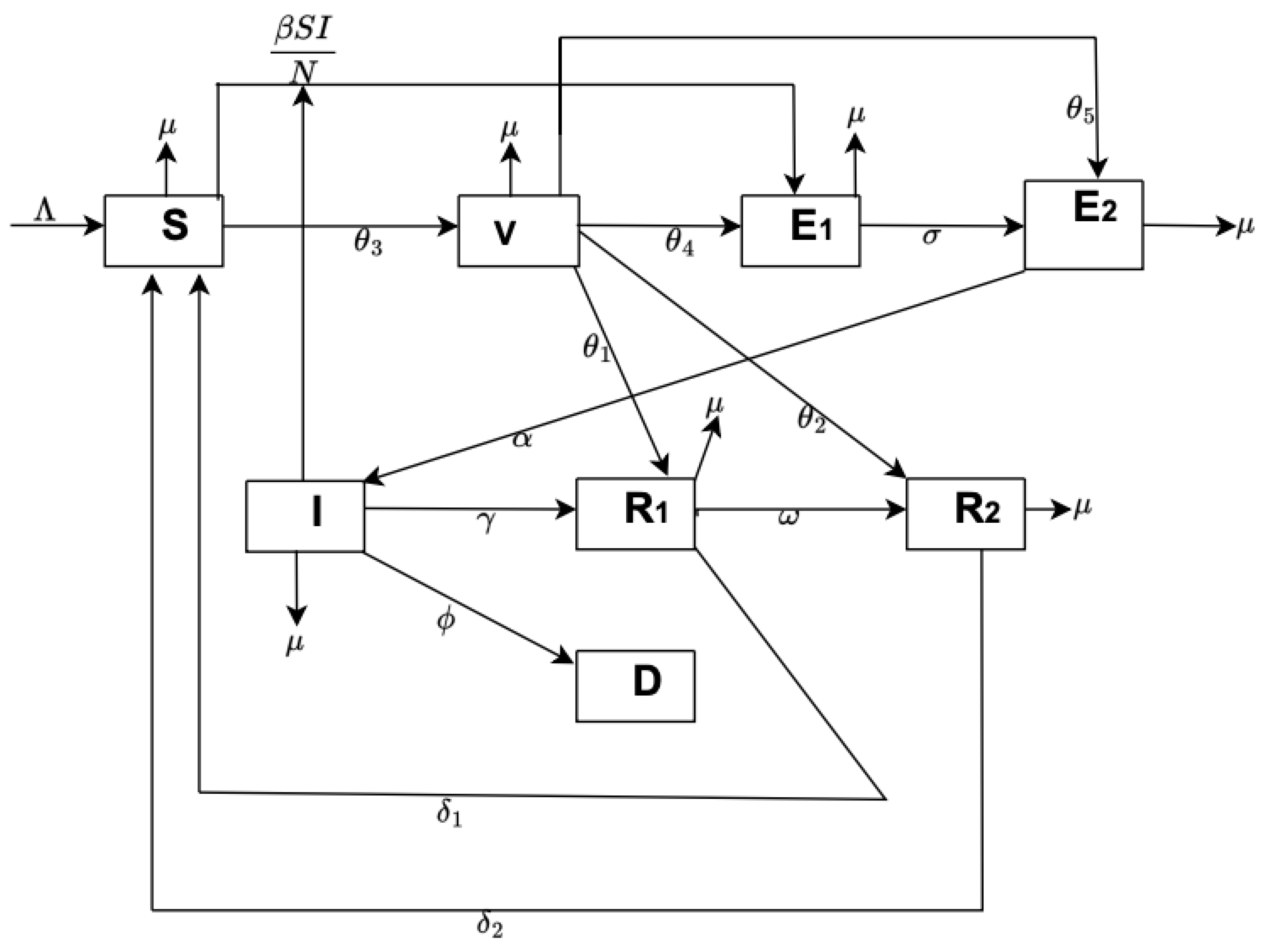
In this section, we propose a mathematical compartmental transmission model for the spread of the COVID-19 outbreak in the UK, consisting of susceptible S ( t ) , vaccinated V ( t ) , exposed unreported E 1 ( t ) , exposed reported E 2 ( t ) , infected I ( t ) , recovered unreported R 1 ( t ) , recovered reported R 2 ( t ) , and death D ( t ) . The total population ( N ( t ) = S ( t ) + V ( t ) + E 1 ( t ) + E 2 ( t ) + I ( t ) + R 1 ( t ) + R 2 ( t ) + D ( t ) ) is assumed to be very large and open (natural deaths and exit rates are included). Recruitment into susceptible is at rate Λ , β is the effective contact rate, and β S I N is the force of infection. We assumed the entire population (N) had no prior immunity against COVID-19 regardless of their vaccination status and that they can be re-infected. We also assume that some proportion of the vaccinated population can be exposed to the disease and not be reported because they assume that the vaccine makes them immune to the disease. Other parameters are defined in Table 1, and the schematic diagram of the model Equation (1) we developed can be seen in Figure 4. The system of non-linear differential equations for our model is as follows:
d S d t = Λ β S I N θ 3 S μ S + δ 1 R 1 + δ 2 R 2 d V d t = θ 3 S ( θ 4 + θ 5 + μ + θ 1 + θ 2 ) V d E 1 d t = β S I N + θ 4 V ( σ + μ ) E 1 d E 2 d t = σ E 1 + θ 5 V ( α + μ ) E 2 d I d t = α E 2 ( ϕ + γ + μ ) I d R 1 d t = γ I + θ 1 V ( δ 1 + ω + μ ) R 1 d R 2 d t = θ 2 V + ω R 1 ( δ 2 + μ ) R 2 d D d t = ϕ I
where time t > 0 with the initial conditions S ( 0 ) = S 0 0 , V ( 0 ) = V 0 0 , E 1 ( 0 ) = E 10 0 , E 2 ( 0 ) = E 20 0 , I ( 0 ) = I 0 0 , R 1 ( 0 ) = R 10 0 , R 2 ( 0 ) = R 20 0 , D ( 0 ) = D 0 0 .
The mathematical analysis of model (1) such as the positivity, stability, and equilibrium points are presented in Appendix A.

2.3. Statistical Fitting of Model (1)

We used data from a public database from the beginning of the pandemic to July 2022 in the United Kingdom. We used initial values (choice guided by information from [8]) S ( 0 ) = 68,195,416 , V ( 0 ) = 1,000,000 , E 1 ( 0 ) = 60,000 , E 2 ( 0 ) = 50,000 , I ( 0 ) = 20,000 , R 1 ( 0 ) = 15,000 , R 2 ( 0 ) = 10,000 , D ( 0 ) = 5000 for susceptible, vaccinated, exposed unreported, exposed reported, infected, recovered unreported, recovered reported, and recovered individuals in the population, and the values of parameters are in 
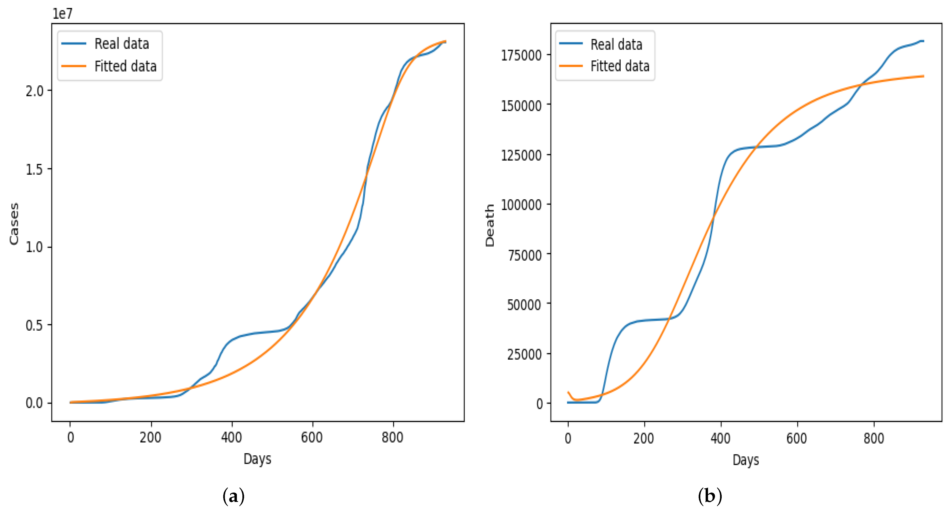
Table 2. Some of the parameters were fitted in order to obtain the optimal parameters, while others were assumed or taken from existing literature. The nonlinear least squares curve fitting technique was used to fit the model to empirical daily case and death data from the UK using the Python programming language, and the graphical result obtained is presented in Figure 5. The result in Figure 5 shows that our model fit the real daily case data better throughout the different phases of the epidemic curve, unlike the fitting presented in Figure 5b in which the dynamics of the fitted data did not capture the real data properly. We also test our model using different partitions of the data before and after vaccination started in the UK, the results of which we did not present in this section. In general, our model fit the daily cases from the beginning of the pandemic up to July 2022 better, as shown in Figure 5a.

2.4. Statistical Predictors and Principal Component Analysis (PCA)

Principal component analysis (PCA) is a technique widely used for dimensionality reduction, feature extraction, and data visualization [19] commonly used in the field of machine learning and statistics. It is used to transform high-dimensional data into a lower-dimensional representation while retaining as much of the original data’s variability as possible. PCA achieves this by finding a set of orthogonal axes, called principal components, along which the data varies the most. The principal component analysis can be applied in the statistical modeling of infectious diseases to help analyze and understand complex datasets related to disease dynamics, transmission patterns, and other epidemiological factors [20]. The first principal component explains the most variance in the data, the second principal component explains the second most, and so on. The k t h principal component of a data (for instance UK COVID-19 cases) vector x ( i ) can therefore be given as a score t k ( i ) = x ( i ) · w ( k ) in the transformed coordinates or as the corresponding vector in the space of the original variables, x ( i ) · w ( k ) w ( k ) , where w ( k ) is the k t h eigenvector of X T X [21].
The distribution of data along its principal components is known as skewness. The distributional characteristics of this data require appropriate preprocessing steps to ensure that PCA results accurately capture the underlying structure of the data. If data contains significant outliers or skewness that cannot be easily addressed through data preprocessing, one might consider using robust PCA techniques that are less sensitive to extreme values and skewed distributions.
Kurtosis, on the other hand, in the context of principal component analysis (PCA), refers to the distribution of data points in terms of their peakedness or the presence of heavy tails in the data’s probability distribution. It measures the degree to which the data deviates from a normal distribution (Gaussian distribution). There are several different measures of kurtosis, but they all essentially assess the tails of the distribution relative to a normal distribution. Kurtosis can have an impact on PCA in the following ways: interpretability of principal components, robustness to outliers, data transformation, and so on. If your data exhibits high kurtosis due to extreme outliers, you might consider using robust PCA techniques that are less sensitive to outliers and heavy-tailed distributions. In as much as kurtosis can impact the results of PCA by affecting the distributional characteristics of the data, appropriate data preprocessing techniques and transformations can help address these issues and lead to more reliable and interpretable principal components.
In summary, skewness and kurtosis are both important measures of a distribution’s shape. Skewness measures the asymmetry of a distribution, while kurtosis measures the heaviness of a distribution’s tails relative to a normal distribution [22].
The coefficient of variation (CV) is a statistic used to measure the relative variability or spread of data points in a dataset. It is expressed as a percentage and is calculated as the ratio of the standard deviation ( σ ) to the mean ( μ ) of the data, multiplied by 100 C V = ( σ μ ) × 100 . The coefficient of variation is often used to compare the variation in datasets with different units or scales. A higher CV indicates greater relative variability, while a lower CV indicates less relative variability. The coefficient of variation can be a helpful tool in the context of PCA for data preprocessing, feature selection, and interpreting the significance of individual variables in the principal components. It helps ensure that PCA is applied appropriately, especially when dealing with datasets with varying scales and levels of variability.
In PCA, the concept from information theory that measures the uncertainty or randomness in a dataset or information source is known as entropy. It is used to gain and interpret information and is also useful in making decisions about splitting data at each node in the (decision trees/forests).
In the broader context of data analysis and preprocessing, especially when assessing the normality of data distributions, the Kolmogorov–Smirnov (KS) test is a statistical test used to compare the distribution of a sample data set with a known distribution or to compare two sample data sets. It assesses whether a sample is drawn from a particular distribution, such as a normal distribution [23]. While the KS test itself is not typically used directly within principal component analysis (PCA). It can be used to identify potential outliers.
The first principal component explains the most variance, the second explains the second most, and so on. Measures of variance, such as the eigenvalues of the covariance matrix, are crucial for understanding the importance of each principal component. The measures of dispersion (dispersion index (ID)), particularly variance and explained variance, play a crucial role in the technique of PCA. PCA aims to maximize the variance of the data along its principal components, and the analysis often involves assessing how much variance is retained or explained by each component to make informed decisions about dimensionality reduction.
Further mathematical formulation of these statistical predictors and PCA can be found in [24,25].

3. Basic Reproduction Number

3.1. Derivation of Basic Reproduction Number of Model (1)

We shall compute the reproduction number R 0 using the next generation matrix (NGM) method [4,5]. The basic reproduction number R 0 is the dominant eigenvalue (spectral radius) of the next generation matrix G i.e., R 0 = ρ ( F V 1 ) , where E 1 , E 2 , and I are the disease classes. We shall assemble the matrix for the model (1) by splitting the model into a new infection matrix F and the transfer matrix V. Thus, we have:
F = 0 0 β Λ ( μ + θ 3 ) 0 0 0 0 0 0 ,
and
V = ( σ + μ ) 0 0 σ ( α + μ ) 0 0 α ( ϕ + γ + μ ) .
Then,
V 1 = 1 σ + μ 0 0 σ ( σ + μ ) ( α + μ ) 1 α + μ 0 α σ ( σ + μ ) ( α + μ ) α ( α + μ ) ( ϕ + γ + μ ) 1 ϕ + γ + μ ,
such that
F V 1 = α σ Λ β ( θ 3 + μ ) ( σ + μ ) ( α + μ ) ( ϕ + γ + μ ) α σ β ( θ 3 + μ ) ( α + μ ) ( ϕ + γ + μ ) Λ β ( θ 3 + μ ) ( ϕ + γ + μ ) 0 0 0 0 0 0
To obtain the spectral radius ρ ( F V 1 ) , we need to determine the eigenvalues of the matrix F V 1 . Hence, by calculation, we have the following
λ 1 = λ 2 = 0 and λ 3 = α σ Λ β ( θ 3 + μ ) ( σ + μ ) ( α + μ ) ( ϕ + γ + μ ) .
Therefore
R 0 = α σ Λ β ( θ 3 + μ ) ( σ + μ ) ( α + μ ) ( ϕ + γ + μ ) .

3.2. Time Varying Reproduction Number

It is a known fact that the basic reproduction number varies across the daily count cases, so we plotted an effective time-varying reproduction number and an average effective reproduction number across the data from the beginning of the pandemic to July 2022 in the United Kingdom, which is presented in Figure 6. The Epyestim [26] package in Python was used, which estimates the effective reproduction number from a time series of reported case numbers of epidemics, and the aggregate of these estimates for the reproduction number is obtained by bootstrap aggregation. This helps us understand how the disease is spread across the epidemic period considered.

3.3. Sensitivity Index

Taking the partial derivative of the basic reproduction number with respect to each of its parameters gives the sensitivity analysis. It tells us the parameters that have the greatest impact on the spread of the disease and evaluates how the uncertainty of the parameters can affect the dynamics of the epidemic [27]. The sensitivity index of the basic reproduction number with respect to parameter p is given by:
S p R 0 = R 0 p · p R 0
Five of the sensitivity indices are negative, while others are positive, as can be seen in Table 3. The sensitivity analysis of the basic reproduction number shows that there is a direct relationship between R 0 and the recruitment into the susceptible class, the contact rate, and the progression rate of exposed reported individuals to the infectious class, which is positively correlated. The progression rate of infectious individuals to recovered unreported classes, the progression rate of exposed unreported individuals to exposed reported classes, the natural death rate, the death rate of infectious individuals, and the rate of vaccination have an inverse relation with R 0 ; hence, they are negatively correlated. Table 3 and Figure 7 present the sensitivity indices as they relate to R 0 .
What can be deduced from the sensitivity analysis is that if the rate of vaccination is increased, the threshold parameter R 0 will decrease, which means the spread of the disease will be curtailed.

4. Numerical Simulation

We used the homotopy perturbation method (HPM) for the numerical simulation of model (1). The description and the analytical solution of the method are presented in the Appendix A. We present the numerical simulation of our mathematical model by varying some of the model parameters to see the behaviour of the epidemic curve over an 8-week period. The visualisation of the results of the simulation with varying parameters is presented in Figure 8, Figure 9, Figure 10 and Figure 11.
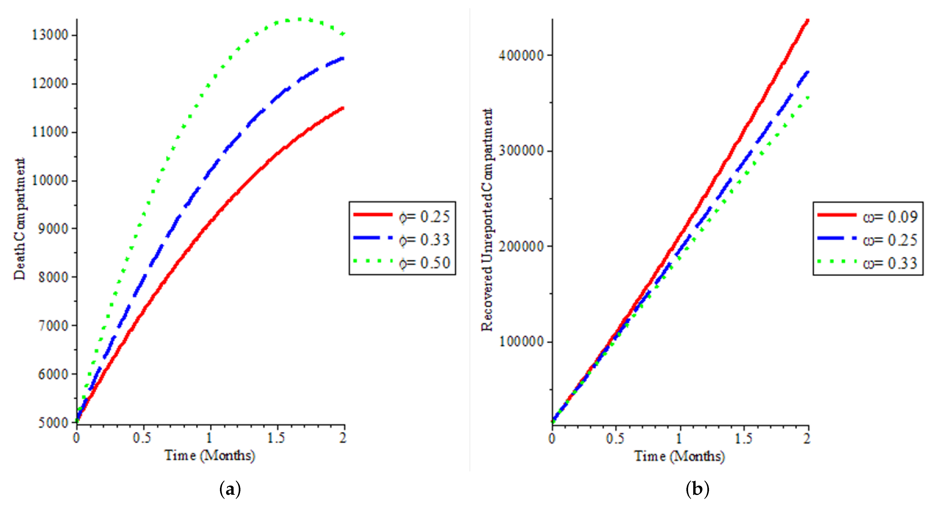
Figure 8a shows that even if we have a high vaccination rate, it does not change the fact that the population is not still susceptible to the COVID-19 virus. It affirms that individuals are not immune to the disease and can be reinfected, which has been the case with COVID-19 dynamics. In Figure 8b, we could say that if more people are exposed to the disease and are infectious, there will be exponential growth in the infected population, which will lead to rapid spread within the population. Figure 9a explains how deaths can be reduced in the population, and our model was able to capture low death rates as observed in the real data of COVID-19 spread in the UK and by extension globally. We demonstrate in Figure 9a that after a time period, most especially when vaccination starts, it can reduce death due to the disease as can be seen in the green line demonstrating a sharp reduction in the death population if we increase the time step. Figure 9b and Figure 10 show that more people recover, whether it is reported or not, if there is an aggressive vaccination campaign leading to more people being vaccinated in the population. This leads to what we have observed in the global COVID-19 recovery count: we have more people recovering from the disease, which is also observed in the UK.
Figure 11a shows that more vaccinated individuals are exposed to the disease and they are unreported, affirming that most COVID-19 cases are unreported while a smaller proportion of the population that is vaccinated and exposed to the disease is reported as shown in Figure 11b.

5. Statistical Modeling and Analysis

5.1. Statistical Analysis of the Entire Dataset

In this section, we present some time-series modeling that is statistically predictive of the evolution of the spread of the COVID-19 outbreak in the UK.
These statistical predictor indicators calculated in a moving window of 14 days are the coefficient of variation (CV), the entropy of the stationary empirical measure, the third and fourth standardized moments of the empirical distribution (respectively, skewness and kurtosis), the uniformity index, which is the index of dispersion (ID), and the normality index, which is the Kolmogorov–Smirnov test (KStest) of adequacy to the normal distribution, showing, respectively, expectation and standard deviation. We normalized the index of dispersion (normalized ID) to remove outliers. Using the principal component analysis (PCA), a score is built from these statistical indicators, and the prediction performance is estimated from the ability to predict the epidemic exponential growth phase.
All the predictor indicators are calculated in the same moving window, respecting the following rules:
  • Choose the same length of moving window for the predictor indicator calculation (14 days).
  • Use the same time step as for moving the window (1 day).
  • Move the window from the start to the end of the COVID-19 outbreak observed between January 2020 and July 2022 for both daily cases and daily deaths.
A way to obtain an important score is to use the first principal component of the principal component analysis (PCA), which explains in general a sufficient percentage of the variance of the daily new cases and deaths from the UK COVID-19 data empirical distribution. In 
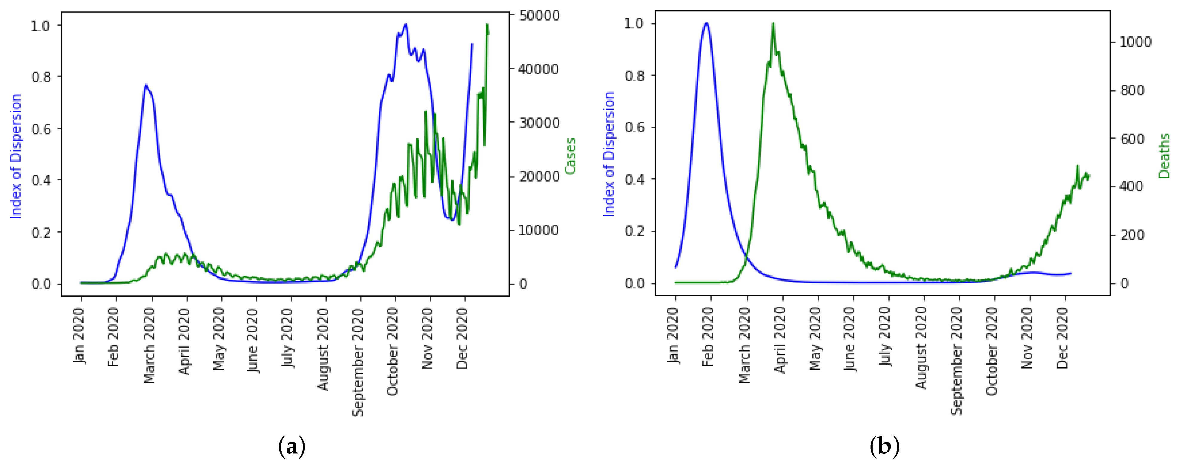
Figure 12, we observe in the UK the evolution of all six statistical predictor indicators for daily new cases and deaths data.
The precision of the forecasting character of both the first PCA principal component, PC0, and the index of dispersion (see Figure 12) can be easily explained by the fact that the ID is often the main weight in the linear combination expressing PC0 on the breakdown coefficients, as calculated for example for the first moving window in the UK daily new cases during early January 2020, the breaking coefficients calculated for the first moving windows of 14 days in Table 4, and the breakdown of principal components (PCs) in Table 5.
P C 0 = 0.000054 K u r t o s i s + 0.0000043 E n t r o p y + 0.0000017 S k e w n e s s + 0.0000063 C V +   1.00 I D + 0.0000000000000031 K S t e s t + 0.00019 N o r m a l i z e d I D .
We plotted ID separately over the daily new cases and deaths because it is the only indicator that captured the disease spread dynamics well as seen in Figure 13a even though there is a shift in the daily death dynamics as shown in Figure 13b. It is not surprising that higher moments like skewness and kurtosis are not capturing the disease dynamics well and have smaller weights in the linear combination of PC0 because it has been statistically proven that higher moments are not good predictor variables.
The epidemic peaks are consistently preceded by the PC0 minima and ID maxima, and therefore it makes sense that the empirical distribution of the new cases has changed (losing stationarity). The index of dispersion ID is, in fact, the logarithm of the ratio between the second and first (mean) moments of the empirical distribution of new cases. Variations in the index of dispersion ID show the loss of stationarity prior to an exponential growth of new cases, which is one of the primary characteristics of the early dynamics of an epidemic peak. The statistical predictors used exhibit the same predicted behavior with PC0. Index of dispersion ID waves take place out of phase with PC0, but they also accurately predict future cases.

5.2. Statistical Analysis before Vaccination Started

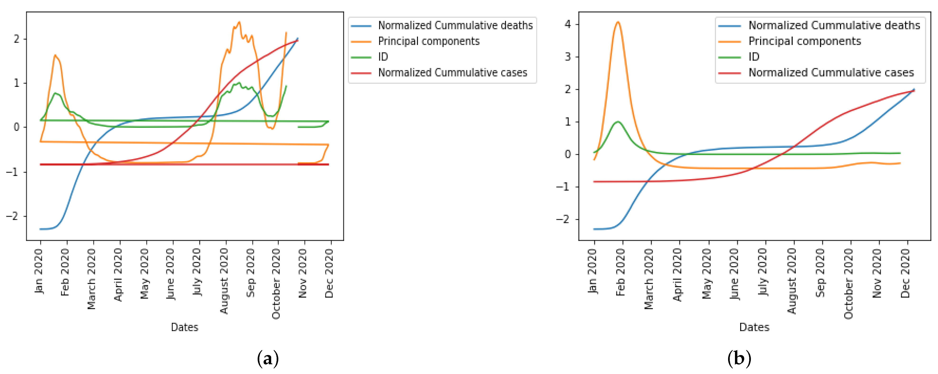
In this section, we present the epidemic dynamics of how these statistical predictor indicators behave before the introduction of vaccination in the population.
In Figure 14, we observe in the UK the evolution of all six statistical predictor indicators for daily new cases and deaths data before vaccination was introduced to the population.
The index of dispersion captured the disease spread dynamics and peaks in the epidemic curve well as seen in Figure 15a even though there is a shift for the daily deaths dynamics as shown in Figure 15b.
In Figure 16, we normalized the cumulative cases and deaths so as to be on the same scale with first principal component and index of dispersion when considering daily new cases and daily deaths before vaccination, respectively, which will help us compare the epidemic waves in the different curves.

5.3. Statistical Analysis after Vaccination Has Started

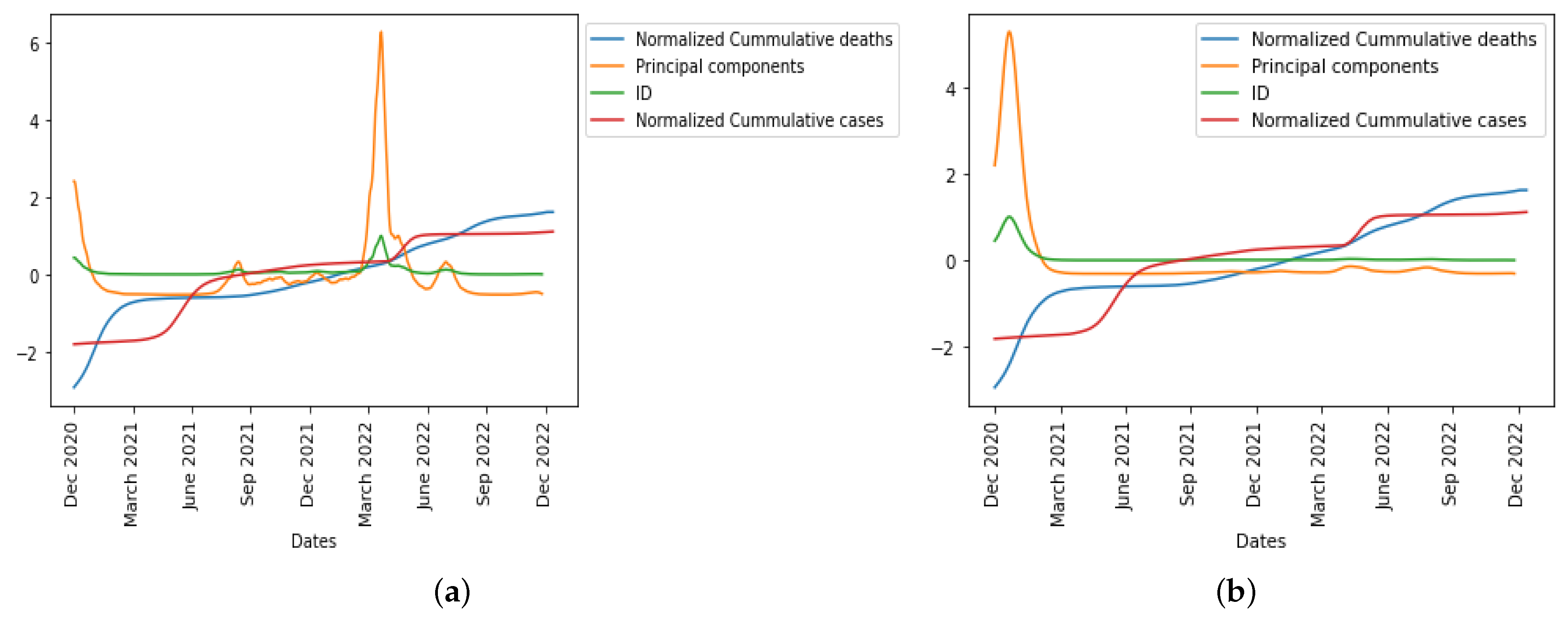
Here, we present the epidemic dynamics of how these statistical predictor indicators behave after vaccination started in the UK.
In Figure 17, we observe in the UK the evolution of all six statistical predictor indicators for daily new cases and deaths data after vaccination was introduced in the population.
The index of dispersion captured the disease spread dynamics and peaks in the epidemic curve well as seen in Figure 18 for both the daily cases and daily deaths. This phenomenon observed in this case might be due to the effect of the vaccination of the population, which enables this statistical predictor indicator to better capture the disease dynamics appropriately.
In Figure 19, we normalized the cumulative cases and deaths so as to be on the same scale with first principal component and index of dispersion when considering daily new cases and daily deaths after vaccination, respectively, which will help us compare the epidemic waves in the different curves.

6. Concluding Remarks

We have shown the nexus between the two approaches we used in this research by predicting the COVID-19 cases and deaths from the beginning of the pandemic in the UK up until July 2022 using a hybrid (mathematical and statistical) model demonstrating high predictive power that shows an alignment with the empirical COVID-19 case and deaths data. The prediction from the fitting of the mathematical model to real data (Figure 5), the simulated results (Figure 8b) that simulated 8 weeks of the epidemic trend, the first principal component curve, and the index of dispersion (see Figure 6b) captured the dynamics of the disease across different exponential and endemic phases in the epidemic curve, showing similarity in trends.
Also, comparing the vaccination trend (see Figure 3) with the results we presented in Figure 17, Figure 18 and Figure 19 explains the influence of vaccination on the epidemic waves (both daily new cases and deaths) after vaccines were introduced to the population.
In this paper, we have been able to use a nonlinear mathematical model to perform some mathematical analysis, fit the model to real data, and also perform some numerical simulation by varying some epidemic parameters. We also calculated the threshold parameter ( R 0 ) and the time-varying R 0 across the pandemic period we considered. We showed the importance of vaccinating individuals in the population, which will help increase recovery among those infected with the virus. Furthermore, we used some statistical predictor indicators to infer how the index of dispersion fit well with the observed data from the UK, used PCA to generate scores, and then used the first principal component, which is the most important in principal component analysis, to capture the trends in the epidemic curve. Our hybrid modeling approach and the consideration of a long epidemic period allow us to demonstrate the robustness of our results, which will be useful for modelers and researchers.
To conclude, the COVID-19 pandemic has been a transformative event with profound implications for global health, society, and the economy. It has challenged us in unprecedented ways but has also brought out our resilience and capacity for innovation. By learning from this experience, we can build a stronger, more equitable world that is better equipped to confront future epidemics. From this paper, we know that integrating mathematical and statistical models with daily empirical case and death data is a valuable approach to understanding and modeling the spread of COVID-19. By combining these two components, researchers and policymakers can gain insights into the dynamics of the disease, enhance the accuracy of models, allow for the estimation of key parameters, predict future trends, evaluate intervention strategies, and facilitate the development of monitoring systems. A future research direction could be considering the age stratification in the UK with the number of doses of vaccine shots received by individuals in the population using a spatial modeling approach at a small spatial scale, which will enable us to understand the local or community spread of the disease and to understand how to deploy resources to mitigate its spread. Another future work could be to look at the disease variants during different peaks of the pandemic and align this with the demographic structure of the population.

Author Contributions

Conceptualization, K.O.; methodology, K.O., O.B., U.M.A., R.T.A. and A.B.Z.; software, K.O., A.J.A., S.A.L., O.A.N., U.M.A., J.O.A. and A.B.Z.; validation, K.O., O.B., A.B.Z. and J.O.A.; formal analysis, U.M.A., O.A.N., K.M.A., O.B., R.T.A. and A.B.Z.; investigation, K.O., O.B., A.B.Z. and J.O.A.; resources, K.O.; data curation, K.O., O.A.N., S.A.L., A.J.A. and U.M.A.; writing and original draft preparation, K.O., U.M.A., R.T.A., J.O.A. and A.B.Z.; writing—review and editing, J.O.A., K.M.A., O.B. and K.O.; visualization, K.O., S.A.L., O.A.N., A.J.A., U.M.A., J.O.A. and A.B.Z.; supervision, K.O.; project administration, K.O. All authors have read and agreed to the published version of the manuscript.

Funding

This research received no external funding.

Data Availability Statement

The data used for this research are available in public databases.

Acknowledgments

This paper is dedicated to Jacques Demongeot for his outstanding contributions to infectious disease modeling.

Conflicts of Interest

The authors declare no conflicts of interest.

Appendix A

Appendix A.1. Mathematical Analysis of Model (1)

Appendix A.1.1. Positivity of Model (1)

 Theorem A1.
Let S ( 0 ) = S 0 , V ( 0 ) = V 0 , E 1 ( 0 ) = E 10 , E 2 ( 0 ) = E 20 , I ( 0 ) = I 0 , R 1 ( 0 ) = R 10 , R 2 ( 0 ) = R 20 and D ( 0 ) = D 0 be the initial values of the state variables. Thus, if S 0 , V 0 , E 10 , E 20 , I 0 , R 10 , R 20 and D 0 are positive, then it implies that S ( t ) , V ( t ) , E 1 ( t ) , E 2 ( t ) , I ( t ) , R 1 ( t ) , R 2 ( t ) and D ( t ) are positive for all t > 0 .
Proof. 
Suppose S 0 , V 0 , E 10 , E 20 , I 0 , R 10 , R 20 and D 0 are positive, then we want to show that the state variables S ( t ) , V ( t ) , E 1 ( t ) , E 2 ( t ) , I ( t ) , R 1 ( t ) , R 2 ( t ) and D ( t ) are positive for all t > 0 . From the model (1), we have
d S d t = Λ β S I N θ 3 S μ S + δ 1 R 1 + δ 2 R 2
which can be re-written as
d S d t + β I N + θ 3 + μ S = Λ + δ 1 R 1 + δ 2 R 2
This implies
d S d t + β I N + θ 3 + μ S 0
d S d t + β I N + θ 3 + μ S 0 d S S β I N + θ 3 + μ d t S ( t ) S ( 0 ) exp β I N + θ 3 + μ t
Since S ( 0 ) = S 0 > 0 , then S ( t ) 0 , for all t > 0 , which is also true for other state variables, which shows that V ( t ) , E 1 ( t ) , E 2 ( t ) , I ( t ) , R 1 ( t ) , R 2 ( t ) and D ( t ) are positive for all t > 0 . □

Appendix A.1.2. Equilibrium Points

Here, we shall discuss both the COVID-19 free equilibrium ( E 0 ) and the endemic equilibrium ( E 1 ) .
Disease Free Equilibrium
The COVID-19 free equilibrium E 0 = S * , V * , E 1 * , E 2 * , I * , R 1 * , R 2 * , D * is defined as the point at which no disease is present within the population, which implies that all the exposed and infected class will be zero.
Thus, the disease free equilibrium for COVID-19 satisfies
E 0 ( κ 0 ) : Λ ( μ + θ 3 ) , θ 3 Λ ( μ + θ 3 ) ( μ + θ 1 + θ 2 + θ 4 + θ 5 ) , 0 , 0 , 0 , 0 , 0 , 0
Endemic Equilibrium
Let E 1 = S * * , V * * , E 1 * * , E 2 * * , I * * , R 1 * * , R 2 * * , D * * be defined as the point where there is still COVID-19 within the population, which implies that all the infected class are nonzero. Then, the equilibrium state under the scenario known as the endemic equilibrium is obtained as:
S * * = σ 2 σ 1 ( μ + θ 1 + θ 2 + θ 4 + θ 5 , V * * = σ 2 σ 1 θ 3 , E 1 * * = Λ μ 2 θ 3 θ 4 + Λ δ 1 δ 2 θ 3 θ 4 + Λ δ 1 μ θ 3 θ 4 + Λ δ 2 μ θ 3 θ 4 + Λ δ 2 ω θ 3 θ 4 + Λ μ ω θ 3 θ 4 ( μ + σ ) σ 1 , E 2 * * = 1 ( α + μ ) ( μ + σ ) σ 1 ( Λ μ 3 θ 3 θ 5 + Λ δ 1 μ 2 θ 3 θ 5 + Λ δ 2 μ 2 θ 3 θ 5 + Λ μ 2 ω θ 3 θ 5 + Λ μ 2 σ θ 3 θ 4 + Λ μ 2 σ θ 3 θ 5 + Λ δ 1 δ 2 μ θ 3 θ 5 + Λ δ 1 δ 2 σ θ 3 θ 4 + Λ δ 1 δ 2 σ θ 3 θ 5 + Λ δ 2 μ ω θ 3 θ 5 + Λ δ 1 μ σ θ 3 θ 4 + Λ δ 1 μ σ θ 3 θ 5 + Λ δ 2 μ σ θ 3 θ 4 + Λ δ 2 μ σ θ 3 θ 5 + Λ δ 2 ω σ θ 3 θ 4 + Λ δ 2 ω σ θ 3 θ 5 + Λ μ ω σ θ 3 θ 4 + Λ μ ω σ θ 3 θ 5 ) I * * = Λ δ 1 μ σ θ 3 θ 5 + Λ δ 2 μ σ θ 3 θ 4 + Λ δ 2 μ σ θ 3 θ 5 + Λ δ 2 ω σ θ 3 θ 4 + Λ δ 2 ω σ θ 3 θ 5 + Λ δ 1 δ 2 μ θ 3 θ 5 + Λ δ 1 δ 2 σ θ 3 θ 4 μ ( α + μ ) ( μ + σ ) σ 1 , R 1 * * = Λ ( δ 2 θ 1 θ 3 + μ θ 1 θ 3 ) σ 1 , R 2 * * = Λ ( δ 1 θ 2 θ 3 + μ θ 2 θ 3 + ω θ 1 θ 3 + ω θ 2 θ 3 ) σ 1 , D * * = Λ α θ 3 ( δ 2 + μ ) ( μ θ 5 + σ θ 4 + σ θ 5 ) ( δ 1 + μ + ω ) ( μ ( α + μ ) ( μ + σ ) σ 1
where
σ 1 = δ 1 μ 3 + δ 2 μ 3 + μ 3 ω + μ 3 θ 1 + μ 3 θ 2 + μ 3 θ 3 + μ 3 θ 4 + μ 3 θ 5 + μ 4 + δ 2 μ 2 ω + δ 1 μ 2 θ 1 + δ 1 μ 2 θ 2 + δ 2 μ 2 θ 1 + δ 1 μ 2 θ 3 + δ 2 μ 2 θ 2 + δ 1 μ 2 θ 4 + δ 2 μ 2 θ 3 + δ 1 μ 2 θ 5 + δ 2 μ 2 θ 4 + δ 2 μ 2 θ 5 + μ 2 ω θ 1 + μ 2 ω θ 2 + μ 2 ω θ 3 + μ 2 ω θ 4 + μ 2 ω θ 5 + μ 2 θ 1 θ 3 + μ 2 θ 2 θ 3 + μ 2 θ 3 θ 4 + μ 2 θ 3 θ 5 + δ 1 δ 2 μ 2 + δ 1 δ 2 μ θ 1 + δ 1 δ 2 μ θ 2 + δ 1 δ 2 μ θ 3 + δ 1 δ 2 μ θ 4 + δ 1 δ 2 μ θ 5 + δ 1 δ 2 θ 3 θ 4 + δ 1 δ 2 θ 3 θ 5 + δ 2 μ ω θ 1 + δ 2 μ ω θ 2 + δ 2 μ ω θ 3 + δ 2 μ ω θ 4 + δ 2 μ ω θ 5 + δ 1 μ θ 2 θ 3 + δ 2 μ θ 1 θ 3 + δ 1 μ θ 3 θ 4 + δ 1 μ θ 3 θ 5 + δ 2 μ θ 3 θ 4 + δ 2 μ θ 3 θ 5 + δ 2 ω θ 3 θ 4 + δ 2 ω θ 3 θ 5 + μ ω θ 1 θ 3 + μ ω θ 2 θ 3 + μ ω θ 3 θ 4 + μ ω θ 3 θ 5 σ 2 = Λ μ 2 + Λ δ 1 δ 2 + Λ δ 1 μ + Λ δ 2 μ + Λ δ 2 ω + Λ μ ω .

Appendix A.1.3. Stability Analysis

To determine the stability of the disease-free equilibrum, we compute the Jacobian matrix of the system (1) and compute the eigenvalues. If all the eigenvalues have a negative real part, then we could say the system is stable. So, the Jacobian matrix evaluated at the disease free equilibrium E 0 is expressed as
J = θ 3 μ 0 0 0 Λ β ( θ 3 + μ ) δ 1 δ 2 0 θ 3 m 2 0 0 0 0 0 0 0 θ 4 ( σ + μ ) 0 Λ β ( θ 3 + μ ) 0 0 0 0 θ 5 σ ( α + μ ) 0 0 0 0 0 0 0 α ( ϕ + γ + μ ) 0 0 μ 0 θ 1 0 0 γ ( δ 1 + ω + μ ) 0 0 0 θ 2 0 0 0 ω ( δ 2 + μ ) 0 0 0 0 0 ϕ 0 0 0
where
m 2 = ( θ 4 + θ 5 + μ + θ 1 + θ 2 ) .
To obtain the eigenvalues, we determine d e t ( J λ I ) = 0 , where
J λ I = θ 3 μ λ 0 0 0 Λ β ( θ 3 + μ ) δ 1 δ 2 0 θ 3 m 2 λ 0 0 0 0 0 0 0 θ 4 ( σ + μ ) λ 0 Λ β ( θ 3 + μ ) 0 0 0 0 θ 5 σ ( α + μ ) λ 0 0 0 0 0 0 0 α ( ϕ + γ + μ ) λ 0 0 μ 0 θ 1 0 0 γ ( δ 1 + ω + μ ) λ 0 0 0 θ 2 0 0 0 ω ( δ 2 + μ ) λ 0 0 0 0 0 ϕ 0 0 λ
From the matrix above, we could observe that since all the parameters are positive, the diagonal element of the matrix is negative. Then, we obtained the eigenvalues of the 8 × 8 matrix, which are given as:
λ 1 = ( θ 3 + μ ) λ 2 = ( ϕ + γ + μ ) λ 3 = ( δ 1 + ω + μ ) λ 4 = ( θ 4 + θ 5 + μ + θ 1 + θ 2 ) λ 5 = ( σ + μ ) ( α + μ ) ( ϕ + γ + μ ) ( α + μ ) 2 ( ϕ + γ + μ ) 2 4 α σ Λ β ( θ 3 + μ ) 2 ( θ 3 + μ ) λ 6 = ( σ + μ ) ( α + μ ) ( ϕ + γ + μ ) + ( α + μ ) 2 ( ϕ + γ + μ ) 2 4 α σ Λ β ( θ 3 + μ ) 2 ( θ 3 + μ ) λ 7 = α σ Λ β ( θ 3 + μ ) ( σ + μ ) ( α + μ ) ( ϕ + γ + μ ) + ( α + μ ) ( σ + μ ) ( ϕ + γ + μ ) δ M 2 ( θ 3 + μ ) λ 8 = α σ Λ β ( θ 3 + μ ) ( σ + μ ) ( α + μ ) ( ϕ + γ + μ ) + ( α + μ ) ( σ + μ ) ( ϕ + γ + μ ) δ + M 2 ( θ 3 + μ )
where
M = ( α + μ ) 2 ( σ + μ ) 2 ( ϕ + γ + μ ) 2 δ 2 α σ Λ β ( θ 3 + μ ) ( σ + μ ) 2 ( α + μ ) 2 ( ϕ + γ + μ ) 2 .
From (A3), we could observe that all the eigenvalues are either negative or have negative real parts. Hence, the disease-free equilibrium is asymptotically stable if:
α σ Λ β ( θ 3 + μ ) ( σ + μ ) ( α + μ ) ( ϕ + γ + μ ) + ( α + μ ) ( σ + μ ) ( ϕ + γ + μ ) δ M 2 ( θ 3 + μ ) < 0
Then,
( α σ Λ β ( θ 3 + μ ) ( σ + μ ) ( α + μ ) ( ϕ + γ + μ ) + ( α + μ ) ( σ + μ ) ( ϕ + γ + μ ) δ M ) < 0 ( α σ Λ β ( θ 3 + μ ) ( σ + μ ) ( α + μ ) ( ϕ + γ + μ ) < ( α + μ ) ( σ + μ ) ( ϕ + γ + μ ) δ + M ( α σ Λ β ( θ 3 + μ ) ( σ + μ ) ( α + μ ) ( ϕ + γ + μ ) < 0 α σ Λ β < ( θ 3 + μ ) ( σ + μ ) ( α + μ ) ( ϕ + γ + μ )
which implies that
α σ Λ β ( θ 3 + μ ) ( σ + μ ) ( α + μ ) ( ϕ + γ + μ ) < 1
Hence,
R 0 < 1 .

Appendix A.1.4. Analytical Solution of Model (1) Using Homotopy Perturbation Method (HPM)

The homotopy perturbation method (HPM) was first discovered by the author in [28]. The homotopy perturbation method (HPM), which provides an analytically approximate solution, is applied to various linear and non-linear equations. The homotopy perturbation method (HPM) is a series expansion method used in the solution of nonlinear partial differential equations. Given the initial conditions:
S ( 0 ) = S 0 , V ( 0 ) = V 0 , E 1 ( 0 ) = E 10 , E 2 = E 20 , I ( 0 ) = I 0 , R 1 ( 0 ) = R 10 , R 2 ( 0 ) = R 20 , D ( 0 ) = D 0
Let
S = a 0 + h a 1 + h 2 a 2 + V = b 0 + h b 1 + h 2 b 2 + E 1 = c 0 + h c 1 + h 2 c 2 + E 2 = d 0 + h d 1 + h 2 d 2 + I = e 0 + h e 1 + h 2 e 2 + R 1 = f 0 + h f 1 + h 2 f 2 + R 2 = g 0 + h g 1 + h 2 g 2 + D = n 0 + h n 1 + h 2 n 2 +
Applying HPM to (1), we obtain the following equations.
h 0 : a 0 1 = 0 h 1 : a 1 + K a 0 e 0 + ( θ 3 + μ ) a 0 δ 1 f 0 δ 2 g 0 Λ = 0 h 2 : a 2 + K ( a 0 e 1 + a 1 e 0 ) + ( θ 3 + μ ) a 1 δ 1 f 0 δ 2 g 0 = 0
h 0 : b 0 1 = 0 h 1 : b 1 + ( θ 4 + θ 5 + θ 1 + θ 2 + μ ) b 0 θ 3 a 0 = 0 h 2 : b 2 + ( θ 4 + θ 5 + θ 1 + θ 2 + μ ) b 1 θ 3 a 1 = 0
h 0 : c 0 = 0 h 1 : c 1 + ( σ + μ ) c 0 θ 4 b 0 K a 0 e 0 = 0 h 2 : c 2 + ( σ + μ ) c 1 θ 4 b 1 K ( a 0 e 1 + a 1 e 0 ) = 0
h 0 : d 0 = 0 h 1 : d 1 + ( α + μ ) d 0 σ c 0 θ 5 b 0 = 0 h 2 : d 2 + ( α + μ ) d 1 σ c 1 θ 5 b 1 = 0
h 0 : e 0 = 0 h 1 : e 1 + ( ϕ + γ + μ ) e 0 α d 0 = 0 h 2 : e 2 + ( ϕ + γ + μ ) e 0 α d 1 = 0
h 0 : f 0 = 0 h 1 : f 1 + ( ω + δ 1 + μ ) f 0 θ 1 b 0 γ e 0 = 0 h 2 : f 2 + ( ω + δ 1 + μ ) f 1 θ 1 b 1 γ e 1 = 0
h 0 : g 0 = 0 h 1 : g 1 + ( δ 2 + μ ) g 0 θ 2 b 0 ω f 0 = 0 h 2 : g 2 + ( δ 2 + μ ) g 1 θ 2 b 1 ω 1 f 1 = 0
h 0 : n 0 = 0 h 1 : n 1 ϕ e 0 = 0 h 2 : n 2 ϕ e 1 = 0
Solving (A7)–(A14) by direct integrating method for h 0 , we obtain the following
a 0 = S 0 b 0 = V 0 c 0 = E 10 d 0 = E 20 e 0 = I 0 f 0 = R 10 g 0 = R 20 n 0 = D 0
where S 0 , V 0 , E 10 , E 20 , I 0 , R 10 , R 20 , D 0 are all constants.
Substituting (A15) into (A7)–(A14) and solving by direct integration method for h 1 , we obtain the following equations.
a 1 = Λ + δ 2 R 20 + δ 1 R 10 K S 0 I 0 ( θ 3 + μ ) S 0 t b 1 = θ 3 S 0 ( μ + θ 2 + θ 1 + θ 5 + θ 4 ) V 0 t c 1 = K S 0 I 0 + θ 4 V 0 ( μ + σ ) E 10 t d 1 = θ 5 V 0 + σ E 10 ( μ + α ) E 20 t e 1 = α E 20 ( γ + μ + ϕ ) I 0 t f 1 = γ I 0 + θ 1 V 0 ( ω + δ 1 + μ ) R 10 t g 1 = ω R 10 + θ 2 R 20 ( δ 2 + μ ) R 20 t n 1 = ϕ I 0 t
Similarly, substituting (A15) and (A16) into (A7)–(A14) and solving by direct integration for h 2 , we obtain the following equations.
a 2 = δ 2 ( θ 2 R 20 + ω R 10 ( μ + δ 2 ) R 20 ) + δ 1 ( γ I 0 + θ 1 V 0 ( μ + ω + δ 1 ) R 10 ) ( θ 3 + μ ) ( Λ + δ 2 R 20 + δ 1 R 10 ( θ 3 + μ ) S 0 K S 0 I 0 ) K ( Λ + δ 2 R 20 + δ 1 R 10 ( θ 3 + μ ) S 0 K S 0 I 0 ) I 0 K S 0 ( α E 20 ( γ + ϕ + μ ) I 0 ) t 2 2
b 2 = θ 3 ( Λ + δ 2 R 20 + δ 1 R 10 ( θ + μ ) S 0 K S 0 I 0 ) ( θ 4 + θ 5 + θ 1 + θ 2 + μ ) ( θ 3 S 0 ( θ 4 + θ 5 + θ 1 + θ 2 + μ ) V 0 ) t 2 2
c 2 = K ( Λ + δ 2 R 20 + δ 1 R 10 ( θ 3 + μ ) S 0 K S 0 I 0 ) I 0 + K S 0 ( α E 20 ( γ I 0 μ ϕ I 0 ) I 0 ) + θ 4 ( θ 3 S 0 ( θ 4 + θ 5 + θ 1 + θ 2 + μ ) V 0 ) ( ( σ + μ ) ) ( K S 0 I 0 + θ 4 V 0 ( σ + μ ) E 10 ) t 2 2
d 2 = σ ( K S 0 I 0 + θ 4 V 0 ( σ + μ ) E 10 ) + θ 5 ( θ 3 S 0 ( θ 4 + θ 5 + θ 1 + θ 2 + μ ) V 0 ) ( α + μ ) ( θ 5 V 0 + σ E 10 ( α + μ ) E 20 ) t 2 2
e 2 = α ( θ 5 V 0 + σ E 10 ( α + μ ) E 20 ) ( ϕ + γ + μ ) ( α E 20 ( γ + μ + ϕ ) I 0 ) t 2 2
f 2 = γ ( α E 2 0 ( γ + μ + ϕ ) I 0 ) + θ 1 ( θ 3 S 0 ( θ 1 + θ 2 + θ 4 + θ 5 + μ ) V 0 ) ( ω + δ 1 + μ ) ( γ I 0 + θ 1 V 0 ( ω + δ 1 + μ ) R 10 ) t 2 2
g 2 = θ 2 ( θ 3 S 0 ( θ 1 + θ 2 + θ 4 + θ 5 + μ ) V 0 ) ω ( γ I 0 + θ 1 V 0 ( δ 1 + ω + μ ) R 10 ) ( δ 1 + μ ) ( θ 2 R 20 + ω R 10 ( δ 2 + μ ) R 20 ) t 2 2
n 2 = ϕ ( α E 20 ( γ + μ + ϕ ) I 0 ) t 2 2
But, from (A28), if we let:
lim h 1 S ( t ) = lim h 1 ( a 0 + h a 1 + h 2 a 2 + ) = a 0 + a 1 + a 2 + lim h 1 V ( t ) = lim h 1 ( b 0 + h b 1 + h 2 b 2 + ) = b 0 + b 1 + b 2 + lim h 1 E 1 ( t ) = lim h 1 ( c 0 + h c 1 + h 2 c 2 + ) = c 0 + c 1 + c 2 + lim h 1 E 2 ( t ) = lim h 1 ( d 0 + h d 1 + h 2 d 2 + ) = d 0 + d 1 + d 2 + lim h 1 I ( t ) = lim h 1 ( e 0 + h e 1 + h 2 e 2 + ) = e 0 + e 1 + e 2 + lim h 1 R 1 ( t ) = lim h 1 ( f 0 + h f 1 + h 2 f 2 + ) = f 0 + f 1 + f 2 + lim h 1 R 2 ( t ) = lim h 1 ( g 0 + h g 1 + h 2 g 2 + ) = g 0 + g 1 + g 2 + lim h 1 D ( t ) = lim h 1 ( n 0 + h n 1 + h 2 n 2 + ) = n 0 + n 1 + n 2 +
Then, we have:
S ( t ) = lim h 1 S ( t ) = lim h 1 ( a 0 + h a 1 + h 2 a 2 + ) = a 0 + a 1 + a 2 + S ( t ) = S 0 + ( Λ + δ 2 R 20 + δ 1 R 10 K S 0 I 0 ( θ 3 + μ ) S 0 ) t + δ 2 ( θ 2 R 20 + ω R 10 ( μ + δ 2 ) R 20 ) + δ 1 ( γ I 0 + θ 1 V 0 ( μ + ω + δ 1 ) R 10 ) ( θ 3 + μ ) ( Λ + δ 2 R 20 + δ 1 R 10 ( θ 3 + μ ) S 0 K S 0 I 0 ) K ( Λ + δ 2 R 20 + δ 1 R 10 ( θ 3 + μ ) S 0 K S 0 I 0 ) I 0 K S 0 ( α E 20 ( γ + ϕ + μ ) I 0 ) t 2 2
V ( t ) = lim h 1 V ( t ) = lim h 1 ( b 0 + h b 1 + h 2 b 2 + ) = b 0 + b 1 + b 2 + V ( t ) = V 0 + ( θ 3 S 0 ( μ + θ 2 + θ 1 + θ 5 + θ 4 ) V 0 ) t + θ 3 ( Λ + δ 2 R 20 + δ 1 R 10 ( θ + μ ) S 0 K S 0 I 0 ) ( θ 4 + θ 5 + θ 1 + θ 2 + μ ) ( θ 3 S 0 ( θ 4 + θ 5 + θ 1 + θ 2 + μ ) V 0 ) t 2 2
E 1 ( t ) = lim h 1 E 1 ( t ) = lim h 1 ( c 0 + h c 1 + h 2 c 2 + ) = c 0 + c 1 + c 2 + E 1 ( t ) = E 10 + ( K S 0 I 0 + θ 4 V 0 ( σ μ ) E 10 ) t + K ( Λ + δ 2 R 20 + δ 1 R 10 ( θ 3 + μ ) S 0 K S 0 I 0 ) I 0 + K S 0 ( α E 20 ( γ I 0 μ ϕ I 0 ) I 0 ) + θ 4 ( θ 3 S 0 ( θ 4 + θ 5 + θ 1 + θ 2 + μ ) V 0 ) ( ( σ + μ ) ) ( K S 0 I 0 + θ 4 V 0 ( σ + μ ) E 10 ) t 2 2
E 2 ( t ) = lim h 1 E 2 ( t ) = lim h 1 ( d 0 + h d 1 + h 2 d 2 + ) = d 0 + d 1 + d 2 + E 2 ( t ) = E 20 + ( θ 5 V 0 σ E 10 ( α + μ ) E 20 ) t + σ ( K S 0 I 0 + θ 4 V 0 ( σ + μ ) E 10 ) + θ 5 ( θ 3 S 0 ( θ 4 + θ 5 + θ 1 + θ 2 + μ ) V 0 ) ( α + μ ) ( θ 5 V 0 + σ E 10 ( α + μ ) E 20 ) t 2 2
I ( t ) = lim h 1 I ( t ) = lim h 1 ( e 0 + h e 1 + h 2 e 2 + ) = e 0 + e 1 + e 2 + I ( t ) = I 0 + ( α E 20 ( γ + μ + ϕ ) I 0 ) t + α ( θ 5 V 0 + σ E 10 ( α + μ ) E 20 ) ( ϕ + γ + μ ) ( α E 20 ( γ + μ + ϕ ) I 0 ) t 2 2
R 1 ( t ) = lim h 1 R 1 ( t ) = lim h 1 ( f 0 + h f 1 + h 2 f 2 + ) = f 0 + f 1 + f 2 + R 1 ( t ) = R 10 + ( γ I 0 + θ 1 V 0 ( ω + μ + δ 1 ) R 10 ) t + γ ( α E 2 0 ( γ + μ + ϕ ) I 0 ) + θ 1 ( θ 3 S 0 ( θ 1 + θ 2 + θ 4 + θ 5 + μ ) V 0 ) ( ω + δ 1 + μ ) ( γ I 0 + θ 1 V 0 ( ω + δ 1 + μ ) R 10 ) t 2 2
R 2 ( t ) = lim h 1 R 2 ( t ) = lim h 1 ( g 0 + h g 1 + h 2 g 2 + ) = g 0 + g 1 + g 2 + R 2 ( t ) = R 20 + ( ω R 10 + θ 2 R 20 ) t + θ 2 ( θ 3 S 0 ( θ 1 + θ 2 + θ 4 + θ 5 + μ ) V 0 ) ω ( γ I 0 + θ 1 V 0 ( δ 1 + ω + μ ) R 10 ) ( δ 1 + μ ) ( θ 2 R 20 + ω R 10 ( δ 2 + μ ) R 20 ) t 2 2
D ( t ) = lim h 1 D ( t ) = lim h 1 ( n 0 + h n 1 + h 2 n 2 + ) = n 0 + n 1 + n 2 + D ( t ) = D 0 + ϕ I 0 t + ( ϕ ( α E 20 ( γ + μ + ϕ ) I 0 ) ) t 2 2

References

  1. Gupta, S.K.; Minocha, R.; Thapa, P.J.; Srivastava, M.; Dandekar, T. Role of the Pangolin in Origin of SARS-CoV-2: An Evolutionary Perspective. Int. J. Mol. Sci. 2022, 23, 9115. [Google Scholar] [CrossRef]
  2. Vandoros, S. Excess mortality during the Covid-19 pandemic: Early evidence from England and Wales. Soc. Sci. Med. 2020, 258, 113101. [Google Scholar] [CrossRef] [PubMed]
  3. Yajada, M.; Moridani, M.K.; Rasouli, S. Mathematical model to predict COVID-19 mortality rate. Infect. Dis. Model. 2022, 7, 761–776. [Google Scholar] [CrossRef] [PubMed]
  4. Oshinubi, K.; Peter, O.J.; Addai, E.; Mwizerwa, E.; Babasola, O.; Nwabufo, I.V.; Sane, I.; Adam, U.M.; Adeniji, A.; Agbaje, J.O. Mathematical Modelling of Tuberculosis Outbreak in an East African Country Incorporating Vaccination and Treatment. Computation 2023, 11, 143. [Google Scholar] [CrossRef]
  5. Babasola, O.; Kayode, O.; Peter, O.J.; Onwuegbuche, F.C.; Oguntolu, F.A. Time-delayed modelling of the COVID-19 dynamics with a convex incidence rate. Inform. Med. Unlocked 2022, 35, 101124. [Google Scholar] [CrossRef] [PubMed]
  6. Addai, E.; Adeniji, A.; Peter, O.J.; Agbaje, J.O.; Oshinubi, K. Dynamics of Age-Structure Smoking Models with Government Intervention Coverage under Fractal-Fractional Order Derivatives. Fractal Fract. 2023, 7, 370. [Google Scholar] [CrossRef]
  7. Ferguson, N.M.; Laydon, D.; Nedjati-Gilani, G.; Imai, N.; Ainslie, K.; Baguelin, M.; Bhatia, S.; Boonyasiri, A.; Cucunubá, Z.; Cuomo-Dannenburg, G.; et al. Report 9: Impact of Non-Pharmaceutical Interventions (NPIs) to Reduce COVID-19 Mortality and Healthcare Demand. Imperial College COVID-19 Response Team. 2020. Available online: https://www.semanticscholar.org/paper/Report-9%3A-Impact-of-non-pharmaceutical-(NPIs)-to-Ferguson-Laydon/0874966fc2b887ece8ce43d4dd09ec180cb11615 (accessed on 20 January 2024).
  8. Office for National Statistics. Coronavirus (COVID-19) Related Deaths in the UK. Available online: https://www.ons.gov.uk/peoplepopulationandcommunity/birthsdeathsandmarriages/deaths/datasets/coronaviruscovid19relateddeathsbylocalauthoritymarch2020toapril2022 (accessed on 3 April 2023).
  9. Flaxman, S.; Mishra, S.; Gandy, A.; Unwin, H.J.T.; Mellan, T.A.; Coupland, H.; Whittaker, C.; Zhu, H.; Berah, T.; Eaton, J.W.; et al. Estimating the effects of non-pharmaceutical interventions on COVID-19 in Europe. Nature 2020, 584, 257–261. [Google Scholar] [CrossRef] [PubMed]
  10. Bhopal, S.S.; Bagaria, J.; Olabi, B.; Bhopal, R. Children and young people remain at low risk of COVID-19 mortality. Lancet Child Adolesc. Health 2021, 5, e12–e13. [Google Scholar] [CrossRef] [PubMed]
  11. Bernal, J.L.; Andrews, N.; Gower, C.; Gallagher, E.; Simmons, R.; Thelwall, S.; Stowe, J.; Tessier, E.; Groves, N.; Dabrera, G.; et al. Effectiveness of COVID-19 vaccines against the B.1.617.2 variant. medRxiv 2021. [Google Scholar] [CrossRef]
  12. Panovska-Griffiths, J.; Kerr, C.C.; Stuart, R.M.; Mistry, D.; Klein, D.J.; Viner, R.M.; Bonell, C. Determining the optimal strategy for reopening schools, the impact of test and trace interventions, and the risk of occurrence of a second COVID-19 epidemic wave in the UK: A modelling study. Lancet Child Adolesc. Health 2020, 4, 817–827. [Google Scholar] [CrossRef] [PubMed]
  13. Bian, L.; Gao, Q.; Gao, F.; Wang, Q.; He, Q.; Wu, X.; Mao, Q.; Xu, M.; Liang, Z. Impact of the Delta variant on vaccine efficacy and response strategies. Expert Rev. Vaccines 2021, 20, 1201–1209. [Google Scholar] [CrossRef] [PubMed]
  14. Minton, J.; Patalay, P.; Matthay, E.C. Excess mortality in the UK during the COVID-19 pandemic: Age groups and places most affected. Wellcome Open Res. 2021, 6, 215. [Google Scholar]
  15. Hay, J.A.; Kennedy-Shaffer, L.; Kanjilal, S.; Lennon, N.J.; Gabriel, S.B.; Lipsitch, M.; Mina, M.J. Estimating epidemiologic dynamics from cross-sectional viral load distributions. Science 2021, 373, eabh0635. [Google Scholar] [CrossRef] [PubMed]
  16. Oshinubi, K.; Ibrahim, F.; Rachdi, M.; Demongeot, J. Functional data analysis: Application to daily observation of COVID-19 prevalence in France. AIMS Math. 2022, 7, 5347–5385. [Google Scholar] [CrossRef]
  17. Worldometer. Available online: https://www.worldometers.info/coronavirus (accessed on 6 July 2023).
  18. Office for National Statistics. Coronavirus (COVID-19) Latest Insights: Vaccines. Available online: https://www.ons.gov.uk/peoplepopulationandcommunity/healthandsocialcare/conditionsanddiseases/articles/coronaviruscovid19latestinsights/vaccines#deaths-by-vaccination-status (accessed on 26 November 2023).
  19. Jolliffe, I.T. Principal Component Analysis; Springer: New York, NY, USA, 2002. [Google Scholar] [CrossRef]
  20. Duarte, P.; Riveros-Perez, E. Understanding the cycles of COVID-19 incidence: Principal Component Analysis and interaction of biological and socio-economic factors. Ann. Med. Surg. 2021, 66, 102437. [Google Scholar] [CrossRef]
  21. Available online: https://en.wikipedia.org/wiki/Principal_component_analysis (accessed on 6 July 2023).
  22. Available online: https://www.itl.nist.gov/div898/handbook/eda/section3/eda35b.htm#:~:text=Skewness%20is%20a%20measure%20of,relative%20to%20a%20normal%20distribution (accessed on 6 July 2023).
  23. Available online: https://www.itl.nist.gov/div898/handbook/eda/section3/eda35g.htm (accessed on 6 July 2023).
  24. Waku, J.; Oshinubi, K.; Adam, U.M.; Demongeot, J. Forecasting the Endemic/Epidemic Transition in COVID-19 in Some Countries: Influence of the Vaccination. Diseases 2023, 11, 135. [Google Scholar] [CrossRef]
  25. Oshinubi, K. Mathematical and Statistical Modeling of Epidemic Data: Application to the Novel COVID-19 Outbreak. Modeling and Simulation. Ph.D. Thesis, University Grenoble Alpes, Grenoble, France, 2022. [Google Scholar]
  26. Cori, A.; Ferguson, N.M.; Fraser, C.; Cauchemez, S. A New Framework and Software to Estimate Time-Varying Reproduction Numbers During Epidemics. Am. J. Epidemiol. 2013, 178, 1505–1512. [Google Scholar] [CrossRef] [PubMed]
  27. Babasola, O.; Omondi, E.O.; Oshinubi, K.; Imbusi, N.M. Stochastic Delay Differential Equations: A Comprehensive Approach for Understanding Biosystems with Application to Disease Modelling. AppliedMath 2023, 3, 702–721. [Google Scholar] [CrossRef]
  28. He, J.-H. Homotopy Perturbation Method for Bifurcation of Nonlinear Problems. Int. J. Nonlinear Sci. Numer. Simul. 2005, 6, 207–208. [Google Scholar] [CrossRef]
Figure 1. (a) Daily new cases and (b) daily deaths of COVID-19 outbreak in the UK (from [17]) as at year 2023 with 3-day moving average (in blue and yellow, respectively).
Covid 04 00020 g001
Figure 2. (a) Cumulative cases and (b) cumulative deaths with their moving average (in blue) as at July 2022.
Covid 04 00020 g002
Figure 3. Proportion of those aged 12 years and over who have received one, two, or three or more doses of a COVID-19 vaccine in the UK from 10 January 2021 to 31 August 2022 (from [18]).
Covid 04 00020 g003
Figure 4. Schematic diagram of the COVID-19 model.
Covid 04 00020 g004
Figure 5. (a) Graph of fitted cases vs. real COVID-19 cases in the UK from the beginning of the pandemic till 31 July 2022. (b) Graph of fitted deaths vs. real COVID-19 deaths in the UK from the beginning of the pandemic till 31 July 2022.
Covid 04 00020 g005
Figure 6. Graph of (a) time-varying reproduction number and (b) average effective reproduction number.
Covid 04 00020 g006
Figure 7. Graph of parameters and their sensitivity indices.
Covid 04 00020 g007
Figure 8. (a) Susceptible human population against time (t is in months) for various θ 3 and (b) infected human population against time (t is in months) for various α .
Covid 04 00020 g008
Figure 9. (a) Death population against time (t is in months) for various ϕ and (b) recovered unreported human population against time (t is in months) for various ω .
Covid 04 00020 g009
Figure 10. (a) Recovered reported human population against time (t is in months) for various θ 2 and (b) recovered reported human population against time (t is in months) for various ω .
Covid 04 00020 g010
Figure 11. (a) Exposed unreported human population against time (t is in months) for various θ 4 and (b) exposed reported human population against time (t is in months) for various θ 5 .
Covid 04 00020 g011
Figure 12. Various statistical predictor indicators for the COVID-19 pandemic in the UK for (a) daily new cases and (b) daily deaths.
Covid 04 00020 g012
Figure 13. The Index of dispersion (in blue) as a predictor of the epidemic waves for the UK COVID-19 outbreak, with (a) daily new cases superimposed (in green) and (b) daily deaths superimposed (in green).
Covid 04 00020 g013
Figure 14. Various statistical predictor indicators for the COVID-19 pandemic in the UK before vaccination started for (a) daily new cases and (b) daily deaths.
Covid 04 00020 g014
Figure 15. The index of dispersion (in blue) as a predictor of the epidemic waves for the UK COVID-19 outbreak before vaccination was introduced in the population, with (a) daily new cases superimposed (in green) and (b) daily deaths superimposed (in green).
Covid 04 00020 g015
Figure 16. PC0 and ID for (a) new cases and (b) deaths before vaccination.
Covid 04 00020 g016
Figure 17. Various statistical predictor indicators for the COVID-19 pandemic in the UK after vaccination has started for (a) daily new cases and (b) daily deaths.
Covid 04 00020 g017
Figure 18. The index of dispersion (in blue) as a predictor of the epidemic waves for the UK COVID-19 outbreak after vaccination campaign has started, with (a) daily new cases superimposed (in green) and (b) daily deaths superimposed (in green).
Covid 04 00020 g018
Figure 19. PC0 and ID for (a) new cases and (b) deaths after vaccination.
Covid 04 00020 g019
Table 1. Parameter definitions.
ParameterDescription
Λ Recruitment into susceptible
β Effective contact rate
ϕ Death rate of infectious individuals
μ Natural death rate
γ Progression rate of infectious individuals to recovered unreported class
θ 1 Progression rate of vaccinated individuals to recovered unreported class
θ 2 Progression rate of vaccinated individuals to recovered reported class
θ 3 Rate of vaccination
θ 4 Progression rate of vaccinated individuals to exposed unreported class
θ 5 Progression rate of vaccinated individuals to exposed reported class
α Progression rate of exposed reported individuals to infectious class
σ Progression rate of exposed unreported individual to exposed reported class
δ 1 Loss of immunity by unreported recovered individual
δ 2 Loss of immunity by reported recovered individual
ω Progression rate of recovered unreported individual to recovered reported class
Table 2. Parameter values.
ParameterReferencesValuesBest FitUnit
Λ Estimated20,00020,000Fixed
β Estimated 0.1 0.1 1/day
ϕ Assumed 1 4 0.245 1/day
μ Assumed 1 2 0.489 1/day
γ [15] 0.1 0.1 1/day
θ 1 Varied ( 0 , 1 ) 0.67 1/day
θ 2 Varied ( 0 , 1 ) 0.72 1/day
θ 3 Varied ( 0 , 1 ) 0.84 1/day
θ 4 Varied ( 0 , 1 ) 0.51 1/day
θ 5 Varied ( 0 , 1 ) 0.611 1/day
α Fitted 1 2 0.5 1/day
σ Fitted 1 2 0.5 1/day
δ 1 Assumed 0.9 0.91 1/day
δ 2 Assumed 0.1 0.111 1/day
ω Fitted 1 11 0.1 1/day
Table 3. Parameters Sensitivity Index.
Parameters Λ β ϕ μ γ σ α θ 3
Sensitivity Index 1.00 1.00 0.6944 0.1932 0.2778 0.0208 0.0196 0.8333
Table 4. Values of the breakdown coefficients during the first 14-day moving windows (0 to 4).
KurtosisEntropySkewnessCVIDKStestNormalizedID
0 1.560422 2.277053 0.429678 0.744472 8.788635 3.225218 × 10 9 0.000163
1 1.147522 2.368861 0.656162 0.639084 7.410055 1.320401 × 10 11 0.000137
2 0.494423 2.438590 0.913383 0.543306 6.030124 1.320401 × 10 11 0.000110
3 0.607783 2.505568 1.222075 0.441749 4.432511 8.637110 × 10 15 0.000080
4 2.486025 2.569515 1.497753 0.327226 2.676923 1.989779 × 10 23 0.000046
Table 5. Values of the breakdown of PCs during the first 14-day moving windows (0 to 4).
PC0PC1PC2
0 3657.958091 0.418547 0.040527
1 3659.336674 0.259834 0.478428
2 3660.716608 0.073121 1.083968
3 3662.314227 0.725743 2.000770
4 3664.069825 1.998592 3.358590
Disclaimer/Publisher’s Note: The statements, opinions and data contained in all publications are solely those of the individual author(s) and contributor(s) and not of MDPI and/or the editor(s). MDPI and/or the editor(s) disclaim responsibility for any injury to people or property resulting from any ideas, methods, instructions or products referred to in the content.

