
Ionospheric Error Models for Satellite-Based Navigation—Paving the Road towards LEO-PNT Solutions


Electrical Engineering Unit, Tampere University, 33720 Tampere, Finland
*
Authors to whom correspondence should be addressed.
Computers 2024, 13(1), 4; https://doi.org/10.3390/computers13010004
Submission received: 6 November 2023
/
Revised: 10 December 2023
/
Accepted: 18 December 2023
/
Published: 22 December 2023
Abstract
:Low Earth Orbit (LEO) constellations have recently gained tremendous attention in the navigational field due to their larger constellation size, faster geometry variations, and higher signal power levels than Global Navigation Satellite Systems (GNSS), making them favourable for Position, Navigation, and Timing (PNT) purposes. Satellite signals are heavily attenuated from the atmospheric layers, especially from the ionosphere. Ionospheric delays are, however, expected to be smaller in signals from LEO satellites than GNSS due to their lower orbital altitudes and higher carrier frequency. Nevertheless, unlike for GNSS, there are currently no standardized models for correcting the ionospheric errors in LEO signals. In this paper, we derive a new model called Interpolated and Averaged Memory Model (IAMM) starting from existing International GNSS Service (IGS) data and based on the observation that ionospheric effects repeat every 11 years. Our IAMM model can be used for ionospheric corrections for signals from any satellite constellation, including LEO. This model is constructed based on averaging multiple ionospheric data and reflecting the electron content inside the ionosphere. The IAMM model’s primary advantage is its ability to be used both online and offline without needing real-time input parameters, thus making it easy to store in a device’s memory. We compare this model with two benchmark models, the Klobuchar and International Reference Ionosphere (IRI) models, by utilizing GNSS measurement data from 24 scenarios acquired in several European countries using both professional GNSS receivers and Android smartphones. The model’s behaviour is also evaluated on LEO signals using simulated data (as measurement data based on LEO signals are still not available in the open-access community; we show a significant reduction in ionospheric delays in LEO signals compared to GNSS. Finally, we highlight the remaining open challenges toward viable ionospheric-delay models in an LEO-PNT context.
1. Introduction and Motivation
1.1. LEO-PNT versus GNSS
There are currently two main types of commercial satellite constellations in the sky with potential for global navigation in LEO orbits and in Medium Earth Orbit (MEO) orbits. On one hand, there has been a surge in the deployment of LEO satellites by various companies in order to meet the increasing demand for broadband connectivity in recent years [1]. This surge has been favoured by the decreasing costs of launching and designing satellites, making them easier to maintain and replace. LEO satellites orbits spread from 200 km to 2000 km above the Earth’s surface, making them the closest satellites to Earth among all commercial satellites currently in the sky. This proximity allows LEO satellites to provide stronger signals than satellites in MEO or Geo-stationary Orbit (GEO). It also results in higher orbital speeds for LEO satellites, giving them favourable geometry and high availability [2,3], which are highly important for navigation purposes. However, this close orbital distance creates the need for “mega-constellations” (i.e., constellations with hundreds or even thousands of satellites) to provide global coverage. Consequently, the interest in using these satellites for Position, Navigation, and Timing (PNT) and broadband connectivity has risen over the past few years. LEO-PNT can be either used as a replacement for current satellite-based positioning systems, such as GNSS (e.g., in cases where GNSS service is not available, due, for example, to high levels of interference) or, more often, as a complement to GNSS navigation in challenging environments, such as indoors or in urban canyons [2,4,5].
On the other hand, GNSS satellites in MEO orbits have been there for decades, and two of these systems, the European Galileo system and the Chinese Beidou system, are still under development. GNSS, as its name points out, is a collection of satellite constellations designed to provide global navigation services. It is utilized by multiple applications, including transport, land surveying, and agriculture [6]. Currently, four major systems inside GNSS provide PNT solutions: Global Positioning System (GPS) provided by the United States, Galileo provided by the European Union, BeiDou provided by China, and GLONASS provided by Russia [7]. Together, they offer extensive coverage for both professional GNSS receivers and mass-market GNSS receivers found in devices such as smartphones. Currently, most satellites in the GNSS system occupy MEO orbits, which lie between 2000 km and 35,786 km above the Earth’s surface. Such altitudes lead to weak signals received on Earth due to their long transmission distance, atmospheric attenuation, and the possibly challenging environments around the user’s receiver.
As previously mentioned, one of the current research trends is to resolve the challenges in GNSS, such as heavy multipath effects in dense urban and indoor environments, and combat the increasing amount of spoofing and jamming in GNSS bands [8] using LEO satellites as complementary or alternative solutions to GNSS. The main potential advantages of LEO-based PNT solutions are the lower path losses (at comparative carrier frequencies) compared to MEO satellites due to their closer proximity to Earth, the lower costs of launching and maintaining LEO satellites compared to MEO satellites, the faster Doppler shifts that make them more suitable for lower-cost Doppler-based positioning in contrast with the code- and carrier-phase positioning used in GNSS, and the wide availability of LEO satellites in the sky (currently there are a few thousand in various constellations, such as Starlink, OneWeb, Iridium, etc., and this number is forecast to reach a few tens of thousands within the next five years) [4].
A complementary solution based on LEO could be, for example, to have GNSS receivers on board LEO satellites and to enable LEO to rebroadcast GNSS-like signals on other frequency bands [9]. This setup can improve the clock stability in LEO satellites by using GNSS clock as a reference. It can also provide a reliable system for tracking LEO’s position, time, and velocity. In addition, configuring LEO satellites to rebroadcast GNSS-like signals on other frequency bands can help these signals mitigate most atmospheric effects. Furthermore, LEO’s higher signal strength can increase the availability of these signals in hard-to-reach places [4,10,11,12,13]. Studies have also shown a significant improvement in positioning accuracy for users that receive their signals from LEO-augmented GNSS satellites [14,15].
LEO-PNT as an alternative solution to GNSS have also been studied, e.g., in [4,16]. The main research questions in such an approach are how to build an optimal LEO constellation for PNT purposes, as well as what receiver architectures are the most suitable to process LEO signals for accurate and robust PNT solutions.
While the research on GNSS is a mature field, the research on LEO-PNT is a relatively new field that has gained more attention during the past couple of years. Therefore, there are still many open challenges related to LEO-PNT, and some of them are related to finding appropriate models for the various sources of errors, including atmospheric errors, for LEO-PNT signals. There are currently no available LEO-PNT measurements in open access that can be used to validate our model. Therefore, our approach has been to first validate the model with existing GPS data, then infer how such a model would be suitable in LEO context and identify the open challenges in adapting such a model to LEO. The next subsection discusses the various sources of errors in satellite-based positioning and the importance of having suitable ionospheric delay models.
1.2. Sources of Errors in Satellite-Based Positioning
All satellite signals (e.g., from LEO or MEO orbits) encounter various sources of error, leading to decreased precision in the accuracy of their final PNT solution: terrestrial errors, such as multipath delays, receiver clock and hardware errors, and terrestrial interferences; atmospheric errors, such as tropospheric and ionospheric delays; and orbital errors, such as satellite hardware delays and satellite orbital uncertainties.
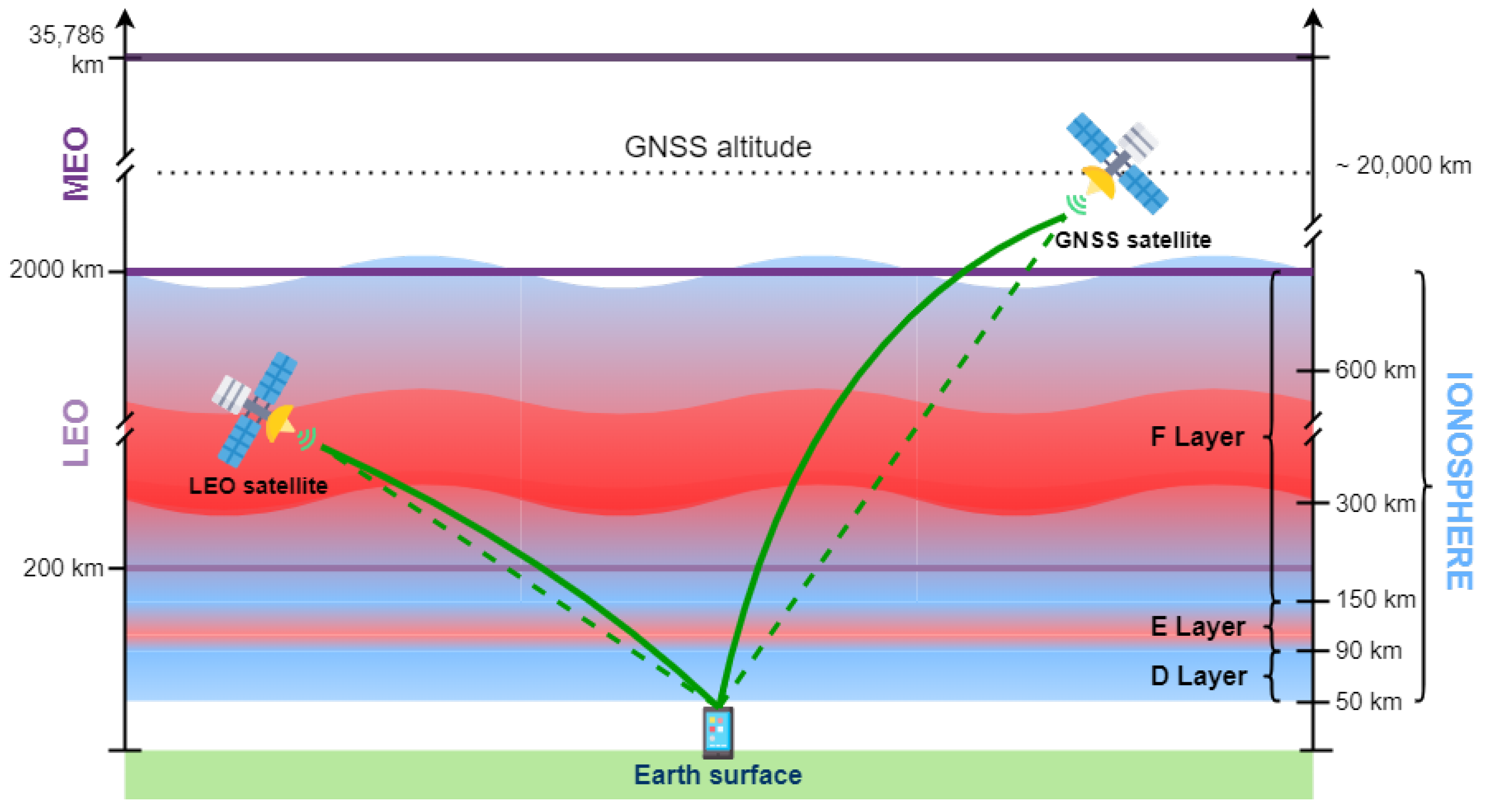
Amongst these multiple sources, ionospheric delay, which is the focus of our paper, stands out as the most significant error source [17,18], at least in all GNSS systems. This delay is induced by the “ionospheric layer”, or simply “ionosphere”, which is a part of the Earth’s atmosphere, ranging approximately from 50 km to 2000 km in altitude [19,20]. Figure 1 represents this region according to its layer description in [21] and with respect to LEO and MEO satellites. The figure also shows how atmospheric layers typically delay the signal by making them follow a path (green line) that is longer than the straight path (dotted green line). The ionospheric layer is typically divided into three sub-layers, D, E, and F, as shown in Figure 1. The most critical region for ionospheric activity is the F layer, shown in bright red in, which spreads from around 300 km to around 600 km above the Earth. The ionosphere can induce positioning errors of up to 100 m on passing signals [22]. Therefore, it is crucial to mitigate its impacts by modelling its effects.
There are several existing models in the literature that aim to mitigate ionospheric delays, such as the NeQuick, Klobuchar, BeiDou Global broadcast Ionospheric delay correction Model (BDGIM), and Quasi-4-Dimension Ionospheric Modeling (Q4DIM) models [23]. These models measure or predict the error induced by the ionosphere, depending on the user’s location, time of day, and day of the year [24,25]. However, all of these models are tailored for correcting errors for GNSS signals and, therefore, cannot be directly applied to signals from LEO satellites. The primary reason for this is the altitude difference between the orbits of the MEO and LEO.
As shown in Figure 1, signals from GNSS satellites penetrate the whole ionosphere, whereas signals from LEO satellites travel only through a portion of it. Furthermore, the topside ionosphere has a greater electron concentration than the bottomside ionosphere, which is around and of the total TEC for the topside and bottomside, respectively [20,26,27]. This indicates that LEO signals experience less interference than GNSS signals. In addition, according to researchers in [28], the topside ionosphere undergoes more significant changes in its electron content than the bottomside ionosphere during solar storms. Hence, the bottomside ionosphere can be considered more stable than the topside ionosphere. This distinction indicates that GNSS signals experience higher ionospheric delay than LEO signals.
1.3. Paper Goals, Research Questions, and Main Contributions
In this paper, we focus on improving the modelling of random ionospheric delays for PNT applications. Therefore, we develop a new model called the Interpolated and Averaged Memory Model (IAMM), which is derived from averaging ionospheric data spanning 11 years, relying on the fact that ionospheric variations have a typical periodicity of 11 years [6,21]. Our model gives us a 2D representation of the electron content inside the ionosphere worldwide based on the solar year, month, and time. In further sections, we give special attention to the LEO-PNT scenario and show the difference in modelling compared to GNSS signals.
The primary focus of our research is to address the following questions. Firstly, how can we develop an ionospheric model that can function offline without requiring correction coefficients to reduce the amount of correction data sent from satellites to ground receivers? Secondly, what is the accuracy gain (or loss) provided by such a model compared to the established ionospheric models that rely on online corrections, such as Klobuchar and IRI models? Finally, how can we expand the GNSS ionospheric models to LEO-PNT systems?
Our paper makes the following key contributions:
- We propose a novel IAMM for ionospheric delay compensation at the receiver;
- We validate the IAMM model by comparing it with current state-of-the-art models used today using real observation data from a variety of GNSS reference stations, as well as from Android mobile receivers;
- We discuss the proposed model’s challenges and possible improvements to the LEO-PNT context.
The rest of the paper is structured as follows: Section 2 gives a brief overview of the main ionospheric delay models in the current literature, with a main focus on GPS signals, which were chosen for our validation campaign. Section 3 describes our methodology and introduces the IAMM model. Section 4 validates the IAMM model with three types of measurement data: data collected by a professional receiver with a fixed roof antenna at our university campus, data available by open access from Finland GNSS reference stations of the FGI network, and data collected via the GNSSlogger app from various mobile devices in dynamic conditions across Europe. A total of 24 scenarios are used (8 per each of the three types mentioned above) for validation purposes. Section 5 discusses the results and how they could be expanded in the context of LEO-PNT, and Section 6 summarizes our findings.
2. Related Work
Current GNSS receivers rely on state-of-the-art models to estimate the ionospheric delay. These models have been developed and refined over time to assess the impact of the ionosphere on GNSS signals, and by utilizing them, GNSS receivers can improve their PNT solution accuracy. Ionospheric models can be categorized into four types: mathematical, empirical, physical, and data-driven. Mathematical models rely on pure mathematical or numerical solutions to provide theoretical values of ionospheric parameters [29,30]. Empirical models represent the ionosphere using equations derived from observational data [31]. Physical models are based on equations that simulate the chemical content and processes governing the ionosphere [31,32]. Data-driven models use multiple methods (e.g., linear regression, autocorrelation, machine learning, neural networks, etc.) to learn from previous observational data to model the ionosphere [33]. We start this section by introducing some key concepts of ionospheric effects before diving into the related work and describing some of the empirical state-of-the-art models.
2.1. Overview of the Ionospheric Delay Concept
The effect of the ionospheric layer on signals has been known for a long time. Even the first satellite-based positioning system included ways to mitigate its impact in their system’s designs. The easiest applicable solution for ionospheric delay compensation is to transmit signals on multiple Radio Frequency (RF) frequencies, as the ionosphere effect is a frequency-dependent delay [24]. Nowadays, high-grade GNSS receivers can track signals from two or more frequency bands and, more recently, some mass-market GNSS receivers are also multi-band receivers [34,35,36,37]. Such receivers are typically called Dual Frequency Receivers (DFRs).
From Equation (6), we can see that the ionospheric delay I is inversely proportional to the carrier frequency . Therefore, the two different frequencies i and j will experience two different delays. DFRs record pseudorange measurements and on the and frequencies, respectively, and then calculate the ionospheric delay corresponding to each frequency using the following formulas:
However, dual-frequency reception requires more advanced hardware (antenna and receiver), which makes it harder to embed DFRs in applications with limited size. Therefore, DFRs are typically used for high-precision receivers, whereas single Frequency Receivers (SFRs) are usually utilized for mass-market GNSS receivers. Note that nowadays, dual-frequency support has been reported even in smartphones [38], yet it still does not concern the majority of smartphones today.
Contrary to DFRs, SFRs rely on two widely used models to estimate ionospheric delay, namely the Klobuchar [23,24,25] and NeQuick [23,25] models. The first is typically used in GPS and BeiDou, while the latter is more encountered in Galileo signals. This is mostly due to how systems provide access to the corrections within their signals [24]. Additional ionospheric models also include IRI, NeQuick2, IGS, BDGIM, etc. [23,39]. Choosing an adequate ionospheric model generally depends on many factors, including real-time availability and computational complexity. In the following subsections, we will discuss the most promising models we found in the literature and their ways of correcting the errors induced by the ionosphere.
2.2. Klobuchar Model
The Klobuchar model was the first model developed to provide ionospheric correction through GPS signals. It is designed to be a computationally lightweight model while delivering a 50% decrease in the RootMean Square (RMS) of the positioning error [23,24,25]. The algorithm, which runs on GNSS receivers, determines the ionospheric delay based on several parameters, such as the user’s approximate geodetic latitude and longitude, elevation and azimuth angles of the visible satellites, and eight coefficients that represent atmospheric parameters and are transmitted within the satellite’s navigation message in GPS and BeiDou signals. It is to be remarked that the validity of these transmitted parameters is only a few hours, which is essentially different from our IAMM model, which has no expiration time. More information about the Klobuchar algorithm can be found in [18,40]. The Klobuchar model is one of the benchmark algorithms we will use in our validation results.
2.3. NeQuick Model
The NeQuick-G model uses empirical and climate-based parameters to represent the ionosphere. It is adopted by Galileo satellites and is designed to remove 70% of ionospheric errors. The NeQuick model has a 3D representation of the electron density inside the ionosphere, and it is able to predict the ionospheric error based on the user’s latitude, longitude, and altitude. This prediction is also based on the coefficients that are broadcast within the Galileo satellite’s navigational message. The NeQuick model is more computationally demanding than other models, such as Klobuchar, but it is also more accurate for Galileo signals [41]. More information about the NeQuick model can be found in [41,42,43]. As our experimental data focus on GPS signals (not on Galileo ones), we have not included the NeQuick model in our benchmark algorithms; addressing Galileo signals remains a topic of future research.
2.4. Neural Network Models
Some ionospheric models use neural networks and machine learning to model the ionosphere. These models are based on data-driven techniques that learn from the historical and observational data of the ionosphere. In [44,45], processing algorithms and measurements from reference stations were used to compute the ionospheric delay at a regional level with high accuracy but with a certain latency. Other research, such as [31], used reference stations along with Machine Learning (ML) algorithms and neural networks to establish accurate values of the ionospheric delay at a regional level. Since there are many neural network-based models in the literature, it has been hard to find a relevant benchmark among them, and therefore, they are not included in our comparisons.
2.5. IRI Model
The IRI is an empirical model designed to provide standardized specifications of plasmaspheric content in the ionosphere. The IRI relies on measurements from rockets, radiowave sounders, and a global network of incoherent scatter radars called “ionosondes” to generate values for the ionospheric composition (e.g., electron densities, temperatures, velocities, ion temperatures, and ion compositions) and Vertical Total Electron Content (VTEC) globally throughout the whole ionosphere and at an altitude range from 60 to 2000 km. One drawback of the IRI model is the irregular distribution of the ionosondes, which can decrease the accuracy of the measurements outside the coverage area of ionosondes, such as the areas over the oceans and across the poles [22]. We refer the readers to [20,46] for a deeper understanding of the model’s architecture and formulation. The IRI-2016 model is taken as one of the comparison benchmarks in our validation analysis.
2.6. IGS Model and Database
The IGS is an organization that has a goal of providing high-quality GNSS data and products. It depends on a collaborative effort of over 200 independent agencies, research facilities, and universities worldwide to provide high-precision data for research purposes. Since its launch in 1994, the IGS has continuously provided an open-access time series of various products with the help of a global network of 450 permanent stations. Such products include clocks and orbits for GNSS and ionospheric and tropospheric products. Several working groups in the IGS are responsible for delivering these products [7].
The Ionosphere Working Group (IWG) is one of these groups tasked with providing ionospheric products. It combines VTEC maps generated by various stations around the world into Global Ionospheric Maps (GIMs), which manifest a global VTEC content of the ionosphere. These maps are generated by analyzing dual-frequency measurements taken by their GNSS stations. According to [39], in 2021, there were eight such stations around the world, called analysis centers. In order to provide GIMs in a standardized format that is easy to exchange, IONosphere map EXchange format (IONEX) has been developed [7].
Currently, the GIMs in IONEX format provided by the IGS come in different types with different latencies depending on the data needed to compute the products:
- Final GIMs (11 days);
- A predicted solution (available 1–2 days in advance).
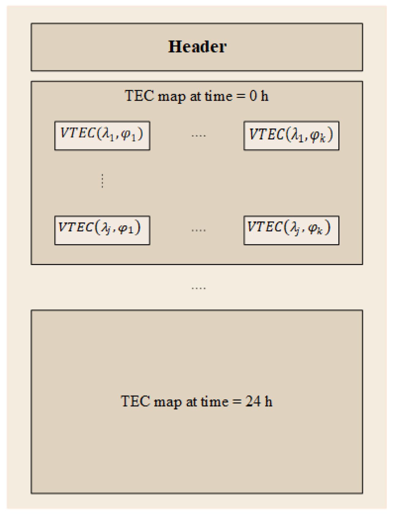
These maps contain, among other information, TEC maps for each epoch (see an explanation in Figure 2, where stands for longitudes and stand for latitudes at point i). These maps are captured at a discrete time every 2 h for 24 h from 00:00 h to 00:00 h the next day, yielding a total of 13 ionospheric maps, each containing TEC values for latitudes
between
and with a spatial resolution of and longitudes between and with a spatial resolution of [48].
Our proposed IAMM model is based on the IONEX data in the IGS database, as explained later in Section 3. Since our model is based on IGS, we did not include IGS as an additional benchmark in our validation results because we believed that this would not bring sufficient added value in the validation process. Instead, we used two external models unrelated to our model to validate the findings (namely, Klobuchar and IRI).
2.7. Ionospheric Models for LEO Satellites
LEO satellites do not have proprietary models to predict the ionospheric delay as GPS and GALILEO satellites have. Due to the orbital height difference between GNSS and LEO satellites, the ionospheric models used for terrestrial receivers need to be modified before they can be applied to LEO satellites. Researchers in [49] used ionospheric data from the IRI model and developed a scale factor to measure the ionospheric delay above an LEO satellite in order to model the ionospheric delay for a GNSS receiver on board an LEO satellite. The authors of [50] used the NeQuick model to calculate the ionospheric delay from a GNSS satellite to a GNSS receiver on board an LEO satellite after they used a scale factor to scale the result from a ground-based to a space-based result. The authors of [51] presented a new communication channel model between an LEO satellite and a ground receiver that takes into account the ionospheric scintillations to analyze the ionospheric effects on bit error rates or channel capacity for satellite communication purposes. However, to the best of the authors’ knowledge, no research so far has tackled the ionospheric delay problem between LEO satellites and the Earth for LEO-PNT applications.
2.8. Summary of State-of-the-Art and Our Proposed Model at a Glance
In Table 1, we present a summary of the reviewed ionospheric models. Our new model Interpolated and Averaged Memory Model (IAMM), to be discussed in Section 3, is also presented and compared in this table for the sake of compactness. The IAMM concept is based on the periodicity of the solar cycle. Assuming that a large part of the ionospheric-related errors are influenced by the solar cycle [19,21], it is possible to predict an averaged delay based on measurements from the previous solar cycle. Each solar cycle lasts for 11 years, and therefore, our model is based on 11 years worth of IONEX files from the IGS database, from the 1 January 2008 to the 31 December 2018. Details on the proposed IAMM methodology and creation will be reviewed in Section 3. The models in Table 1 are discussed based on their type (mathematical, empirical, or data-driven), whether they need broadcast parameters or not, what input data they need to operate, and what kind of output data they deliver.
3. Methodology
The ionosphere is home to atoms and molecules that are directly exposed to the sun’s intense radiation. When these atoms absorb the radiation, many of them lose electrons through a process called ionization [19,21], which causes them to become positively charged as follows:
where A is any molecule or atom in its initial (neutral) state, is the positively charged atom (or ion), and e is the free electron. The ionosphere is packed with these ions and free electrons, hence the term iono.
Fortunately, this absorption process protects humans and other living beings from harmful solar radiation. However, these free electrons inflict considerable delays that affect the propagation of radio waves [21]. That is why ionospheric delay is one of the most significant atmospheric errors that affect RF signals coming from satellites towards the Earth [24,41].
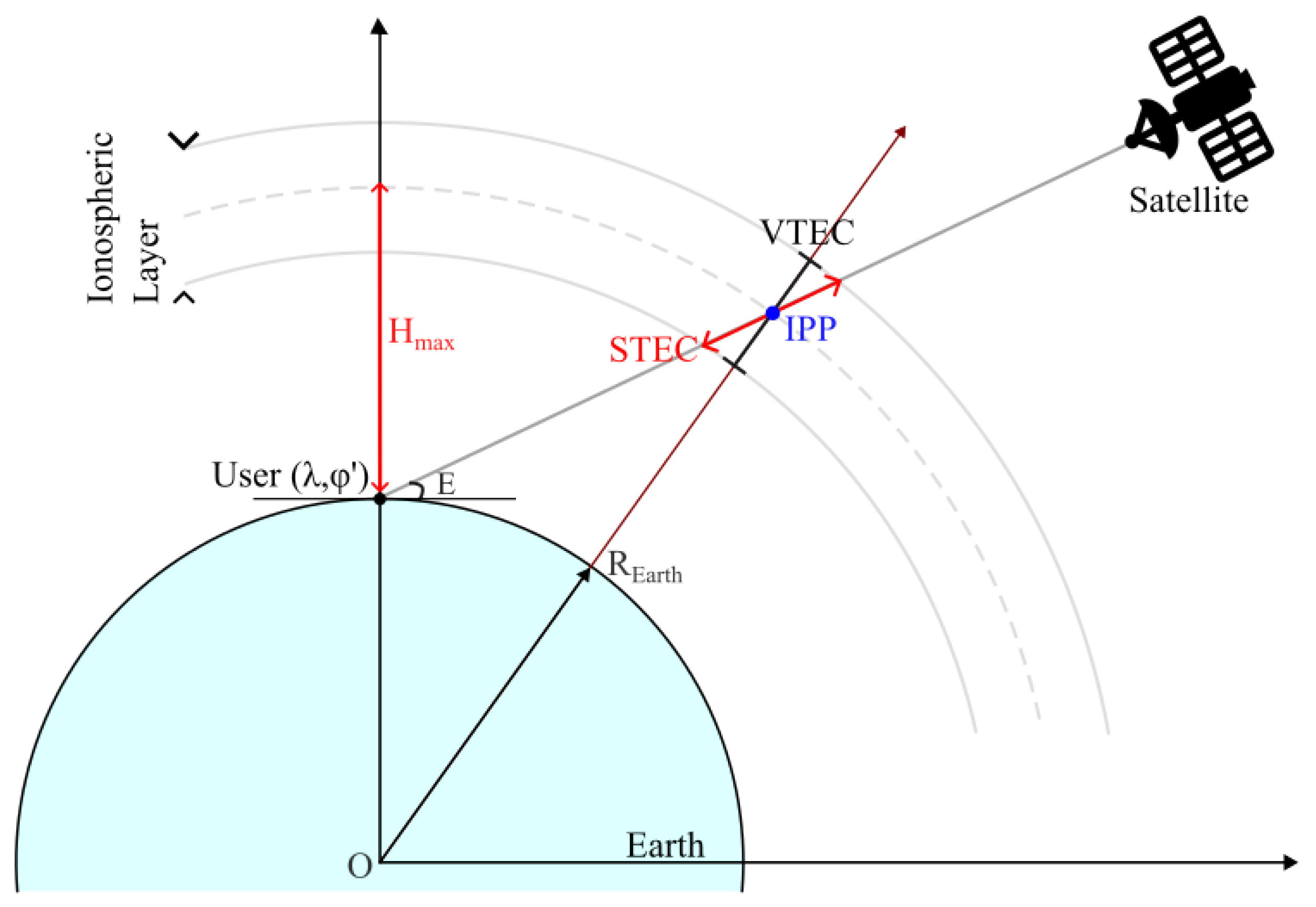
The amount of free electrons in the ionosphere is known as TEC, and it can be of two types: Slant Total Electron Content (STEC), which is the electron content measured along a slanted path, or VTEC, which is the electron content measured at the zenith. Figure 3 highlights the geometric relationship between the two, where are the latitude and longitude of the receiver and is the radius of the Earth. STEC is calculated using the following formula:
where is the number of electrons along path l. The mathematical relationship between STEC and VTEC is given by:
where is the mapping function or the obliquity factor and E is the satellite elevation angle in degrees. There are various mapping functions, but the most common one is the following:
where is the Earth’s radius and is the height of the maximum electron density. Both STEC and VTEC are often expressed in TEC units (TECU), where 1 TECU equals to .
The ionospheric delay corresponding to a satellite’s signal is based on STEC and can be expressed as:
where I is the ionospheric delay in meters, is a constant that is approximately equal to , and is the carrier frequency in Hz. The signal path within the ionosphere increases as the satellite’s elevation angle decreases. This leads to more free electrons intercepting the passing signal, increasing the ionospheric delay.
The ionospheric delay affects the quality of the final positioning solution because it introduces ambiguities to the range calculations that are made by the receiver, known as the pseudorange, which is calculated to determine the user’s position, as shown in Equation (7).
Above, denotes the pseudorange between the satellite and receiver, R represents the true range, I is the ionospheric delay, and represents other delays, such as tropospheric, clock, multipath, and hardware delays.
The main objective is to observe the impact of the ionosphere on an LEO-PNT scenario, so we created a simple ionospheric model that provides a close approximation to the actual ionospheric values using the techniques outlined in [54]. To validate our model, we conducted GPS measurements in various scenarios and compared outputs of the model based on precise measurements from both ground-based GNSS receivers and Android smartphones. In the following sections, we will describe the sources and techniques used to develop the new IAMM model.
3.1. Data Sources
There are several ionospheric models in the literature to choose from in order to simulate the impact of ionospheric delay in our software, as described in Section 2. However, unlike GNSS satellites, LEO satellites do not have designated ionospheric correction models. Therefore, we aimed to derive a model that is not based on transmitted atmospheric data from the satellites. Also, we wanted a model that could function offline without needing a constant connection to a server because this can add significant waiting time to the receiver processing, especially when dealing with thousands of measurements.
The NeQuick and Klobuchar models, while good as a benchmark, do not satisfy our target constraint of having an extensible, file-independent solution that could be used for any satellite constellation or scenario since they rely on broadcasted parameters in ephemeris messages. In our opinion, neural network models are also not highly suitable due to their complexity and regional limitations. The IRI model, which was selected as a second benchmark, has an open-access Matlab implementation. Still, it also requires an online connection to retrieve information about the electron density and TEC content from its server. However, the IONEX files provided by the IGS could fulfil our needs. The IGS was proven to be better than the Klobuchar and NeQuick models in resolving the ionospheric delay for single-frequency receivers [6], and many researchers have tested its accuracy and relied on it as a benchmark to test their model [45,55,56]. For these reasons, we chose to build our model upon the data extracted from the IGS IONEX files.
3.2. Data Collection
The Sun goes through a magnetic cycle every 11 years, influencing the quantity and size of sunspots, solar flares, and Coronal Mass Ejections (CMEs). These factors are indicators of solar activity, and they contribute to a rise in the electron content within the ionosphere [21,57]. The solar cycle commences and ends with a phase of low activity known as the solar minimum, during which the influence on the ionosphere is minimal. The Sun reaches its peak activity level, known as the solar maximum, in the middle of the cycle, during which the impact on the ionosphere increases.
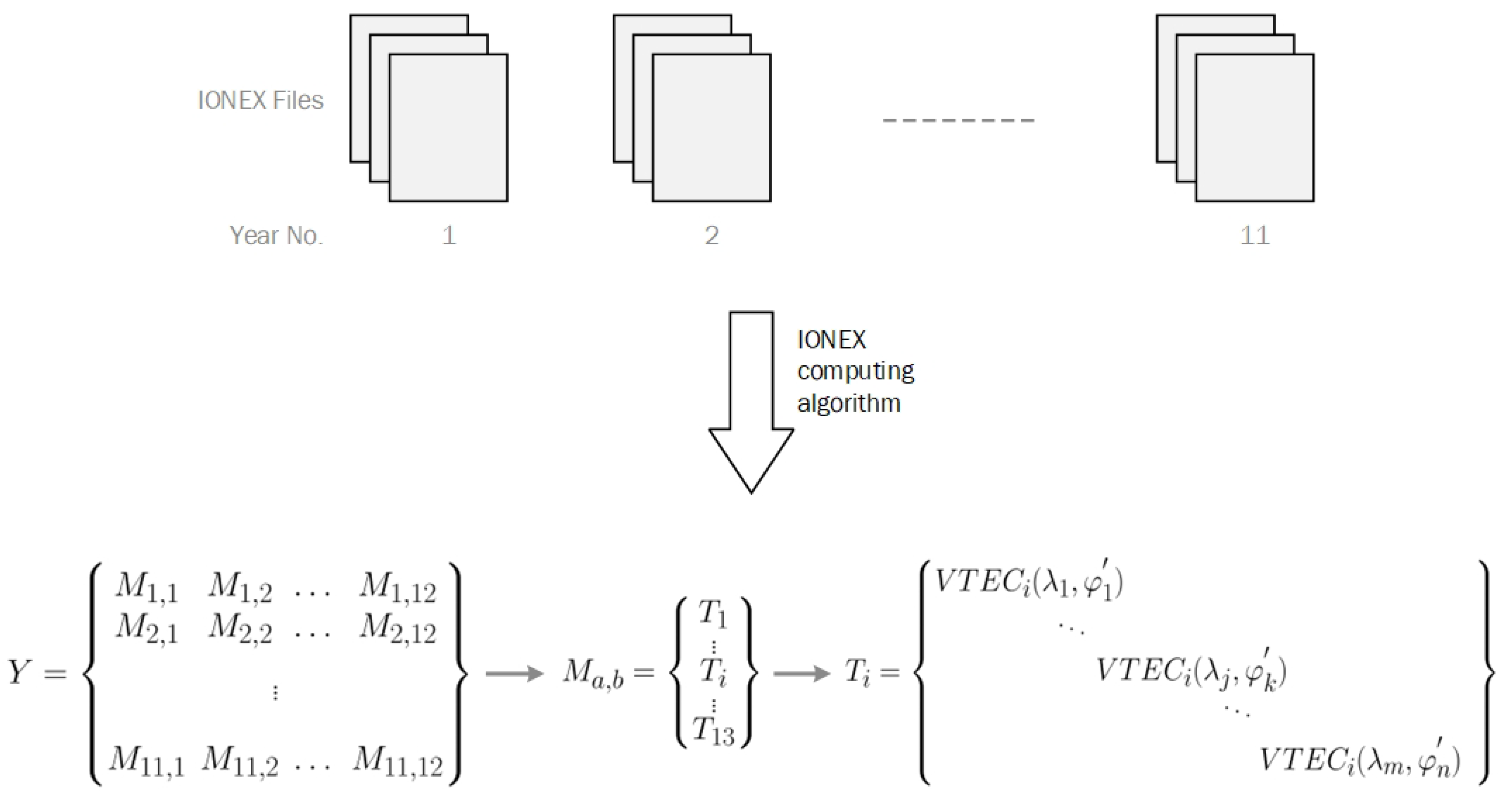
In order to encompass an entire 11-year solar cycle, we collected IONEX files spanning a length of 11 years (2008 to 2018) from the Crustal Dynamics Data Information System (CDDIS) database, which is a database managed by National Aeronautics and Space Administration (NASA) that houses space geodesy data from multiple organizations, such as the IGS. For each month in a year, we collected three IONEX files, giving us a total of 396 files. These files contained the final GIMs, which we chose over other maps for their accuracy.
Next, we used a Matlab code to read all the collected files and generate all the required TEC values, which were then stored in the Y matrix. The data collection and arrangement process is illustrated in Figure 4. The Y matrix has a total number of VTEC values, representing 11 years (one complete solar cycle), 12 months, 13 time instances, 71 latitude values, and 73 longitude values. The year and month data are divided into a set of matrices, where a and b correspond to the year and month, respectively. Every matrix is divided into 13 submatrices, where i represents the time index. These submatrices are arranged systematically, with a 2-h interval between adjacent submatrices. Lastly, every matrix contains a total of VTEC values, corresponding to 71 different latitude values and 73 different longitude values that span the entire Earth with a spatial resolution of degrees for latitudes and 5 degrees for longitudes. This systematic arrangement of data provides a comprehensive representation of VTEC values by latitude, longitude, time of day, month, and year.
It is to be remarked that such a number of parameters can be stored through some compression mechanisms and therefore could occupy below 1 MB of space, or even only a few tens of kB with adequate compression. In addition, as interpolation is further used to obtain exact values at any desired latitude–longitude pair, one can also investigate the situation when we have fewer parameters for the latitude and longitudes than the current 71 and 73 values. This remains a topic for further research.
3.3. IAMM Calculation Strategy
The proposed Interpolated and Averaged Memory Model (IAMM) model uses the averaged data from the Y matrix to generate TEC values. To obtain a TEC value for a specific user at a given date, time, and longitude–latitude location , the IAMM works by first mapping the year of the user into its corresponding solar year. To do that, the year of the user is divided by 11, and then the remainder R of the division is used to map the user’s year to the solar year according to Table 2.
The next step is to interpolate the VTEC values from the matrix. Bilinear interpolation is often used to interpolate values in 2D grids, so we chose bilinear interpolation for our model. It can be performed as follows [7]:
where i is the time index and j and k are the latitude and longitude indices, respectively. The coefficients p and q are calculated across the intervals and , where , being the user’s latitude, is bounded by , which are the surrounding grid points. Similarly, the user’s longitude is bounded by the surrounding grid points and .
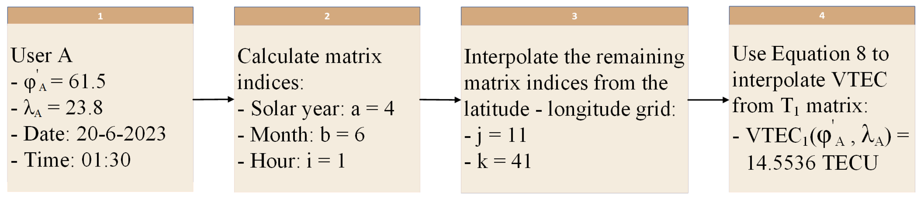
Figure 5 gives a step-by-step example of how the VTEC value of a user is calculated using IAMM. Step 1 tells us that the user is located at Tampere University on 20 June 2023 at 01:30 AM. In step 2, we calculate the solar year based on the user’s year and Table 2, and we calculate other matrix indices corresponding to the user’s date and time. Step 2 tells us that the VTEC value is located in matrix and sub-matrix . To interpolate the VTEC value from the latitude–longitude matrix, we calculate indices j and k based on linear interpolation from the latitude–longitude grid that is defined in the IONEX format datasheet in [7,48]. Finally, in step 4, we use Equation (8) to interpolate the VTEC value for user A from the sub-matrix.
4. Results
4.1. TEC Results
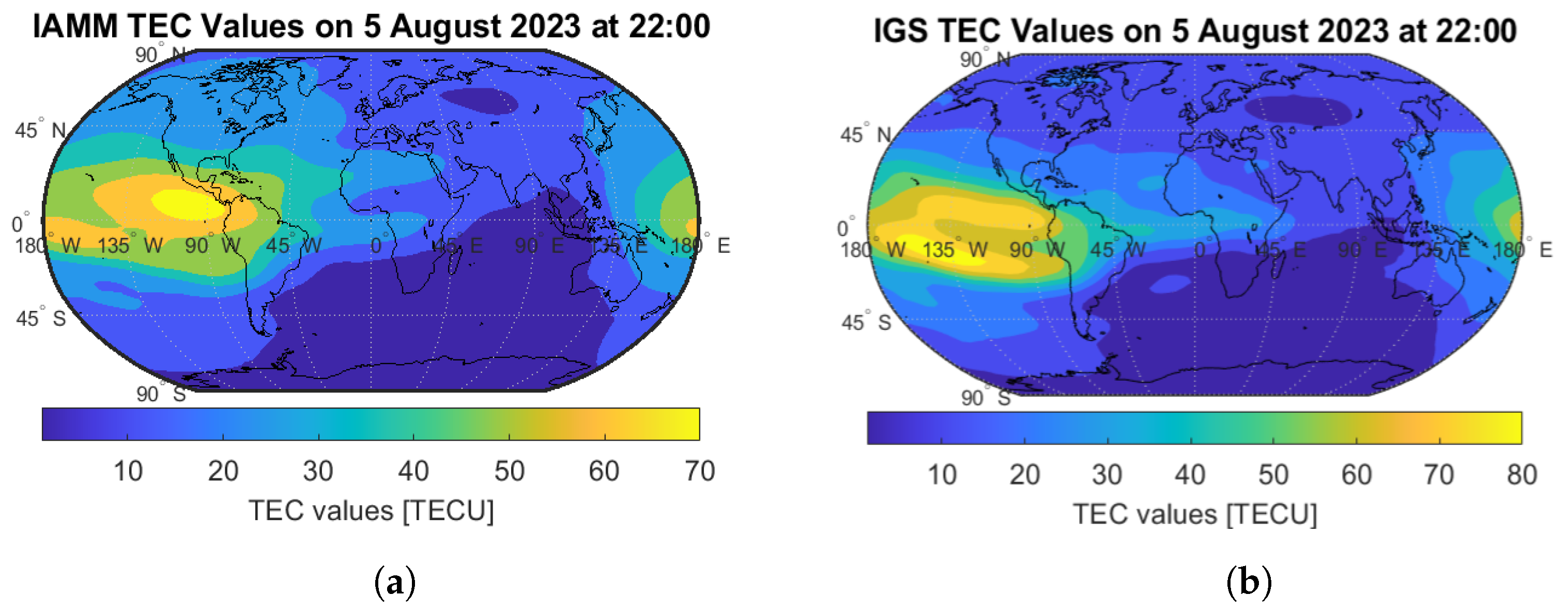
To confirm that our model produced reliable values for ionospheric electron content, we compared the TEC values generated by our IAMM model with those generated by IGS. A snapshot of this comparison is shown in Figure 6a (IAMM) and Figure 6b (IGS) for a period of high solar activity, which happened, for example, to be on 5 August 2023 at around 22:00, according to a report by the National Oceanic and Atmospheric Administration (NOAA) [58]. We chose this date as an illustrative example to show that our model is able to generate reliable TEC values even during periods of intense solar activity. As seen in Figure 6, there is a high similarity between the TEC values generated between the two models.
In order to further verify that our values are close to the real values produced by IGS, we also adopted a statistical approach over several points and computed the correlation coefficients between the two TEC maps, as well as the mean and standard deviation of errors between the two TEC maps (our model versus the IGS model). The results are presented in Table 3. Even with 31098 points, the correlation coefficient between the generated TEC values from the two models is around , which indicates that the TEC map produced by our model follows the same pattern as the TEC map from IGS. Further validation is carried out based on GPS raw measurements in Section 4.2.
4.2. Ionospheric Delay Results
After validating the IAMM model using TEC values, the next step was to verify that the model produces valid ionospheric delay predictions that can improve the positioning accuracy. Consequently, we acquired Receiver Independent Exchange format (RINEX) observation files at various random locations and times from fixed GNSS receivers and from GPS-enabled Android smartphones. Then, we calculated the 3D positioning errors (see Equation (9)) using the four methods below:
- Method 1: No ionospheric correction;
- Method 2: Klobuchar ionospheric correction;
- Method 3: IRI ionospheric correction;
- Method 4: IAMM ionospheric correction.
Methods 1–3 are benchmarks for our proposed model (Method 4).
4.2.1. Data from Reference Stations—Static Conditions
We acquired RINEX observation files from our reference base station at Tampere University (TAU). Note that the absolute location (or ground truth) of the TAU antenna was computed using a Precise Point Positioning (PPP) algorithm and based on five days of data collected from a Septentrio receiver, which is connected to a Talysman roof GNSS antenna.
First, RINEX observation files were acquired from the Septentrio receiver. Next, a Weighted Least Squares (WLS) algorithm following [59] was applied to the observation data. Then, ionospheric corrections were applied following Methods 1–4. Note that we also applied a tropospheric correction model in all four methods (i.e., the dry/hydrostatic Saastamoinen ionospheric model [36]). Finally, we calculated the mean and standard deviation of the 3D positioning error for each method mentioned earlier.
The mean and standard deviation of the 3D positioning error—denoted by and , respectively, with being the scenario index and being the number of scenarios—was computed in x, y, z coordinates in a WGS84 coordinate system via
where are the estimated x, y, z coordinates after the atmospheric delay removal with a weighted least squares approach (following [59]) and are the highly accurate reference positions (obtained via PPP) of the actual roof antenna’s position. The results are presented in Table 4a.
In order to diversify our data origins and further test the models, we also used FINPOS, a service provided by the National Land Survey of Finland (NLS). FINPOS offers various data, including raw observation files from several GNSS base stations across Finland. We collected data from different FINPOS stations at random dates and times and repeated the same process of calculating the 3D positioning error. The results are in Table 4b.
The positioning error means and standard deviations were computed over all tracks of each scenario, where is the total number of measurements for scenario i. The number of scenarios for each of the three cases (i.e., measurements from TAU’s base station, open-access measurements from FINPOS, and measurements collected with the GNSSLogger app from Android phones) was 8 per case, giving us a total of 24 scenarios. The total number of track points per scenario varied, with an average of 28,800, 2883, and 13,699 track points from TAU data, FINPOS data, and Android data, respectively.
is the mean 3D positioning error per scenario i over all tracks and is given by
where
with being the reference (or ground-truth) coordinates and being the estimated coordinates.
is the standard deviation of the 3D positioning error per scenario i over all tracks, defined as 1- (i.e., 68%) of a normal distribution and given by
The final statistics are taken as means and standard deviations averaged over all scenarios :
and
As shown in Table 4, our model performs best when it comes to decreasing the mean of the positioning error induced by the ionosphere for high-grade GNSS receivers (Table 4a,b). The green percentages shown in Table 4 represent the value change for each model with respect to Method 1 (no ionospheric correction).
4.2.2. Data from Android Devices—Dynamic Conditions
Due to the rapid development of GNSS chipsets, Android devices have been extensively used in positioning-related studies in recent years. In 2016, GNSS-equipped Android smartphones made GNSS raw observations available to the public; such raw data can be used to study and interpret positioning accuracy and atmospheric effects. As previously, we collected RINEX observations from these phones in dynamic conditions (phone placed in a moving car, mostly on highways) at various locations (8 locations in Europe) and calculated the resulting positioning errors by applying the same Equations (10) and (12). However, since the exact ground-truth location is no longer available in dynamic conditions, the reference coordinates , and from Equation (11) were taken from National Marine Electronics Association (NMEA) data. NMEA data are estimates produced by the smartphone using its own proprietary algorithms and typically based on GNSS, cellular, and sensor-aided data to generate the best available estimate of the phone’s true position. The statistics were calculated for 8 scenarios collected via the GNSSlogger app from a Nokia XR20 phone in Poland (5 scenarios) and Latvia (2 scenarios) and from a Xiaomi Redmi phone in France (1 scenario).
As shown in Table 4c, the results based on the Android measurements differ from the results based on fixed reference stations, and they show that the Klobuchar model has the best performance, followed by our IAMM model and then the IRI model. The Klobuchar model decreased the positioning error mean and standard deviation by and , respectively. Our model came next in reducing the error mean by and error standard deviation by . Finally, the IRI model reduced the error mean and standard deviation by and , respectively, with respect to the no-correction case.
It is evident that the positioning errors of Android devices from all models are considerably worse than those obtained from GNSS reference stations (Table 4a,b). Several things can explain this increased inaccuracy. First of all, there are many fluctuations and biases in the smartphone’s components [38]. Secondly, dynamic conditions of Android-based measurements may suffer more errors compared to static acquisition. Finally,) the ground-truth position was not available in Android phones; the reference track in there was the NMEA track, which is itself prone to errors (see additional explanations concerning Figure 7 in the next section). We remark that when it comes to positioning, a device explicitly designed for GNSS monitoring will provide much greater accuracy than a smartphone.
4.3. Results Extended to an LEO-PNT System
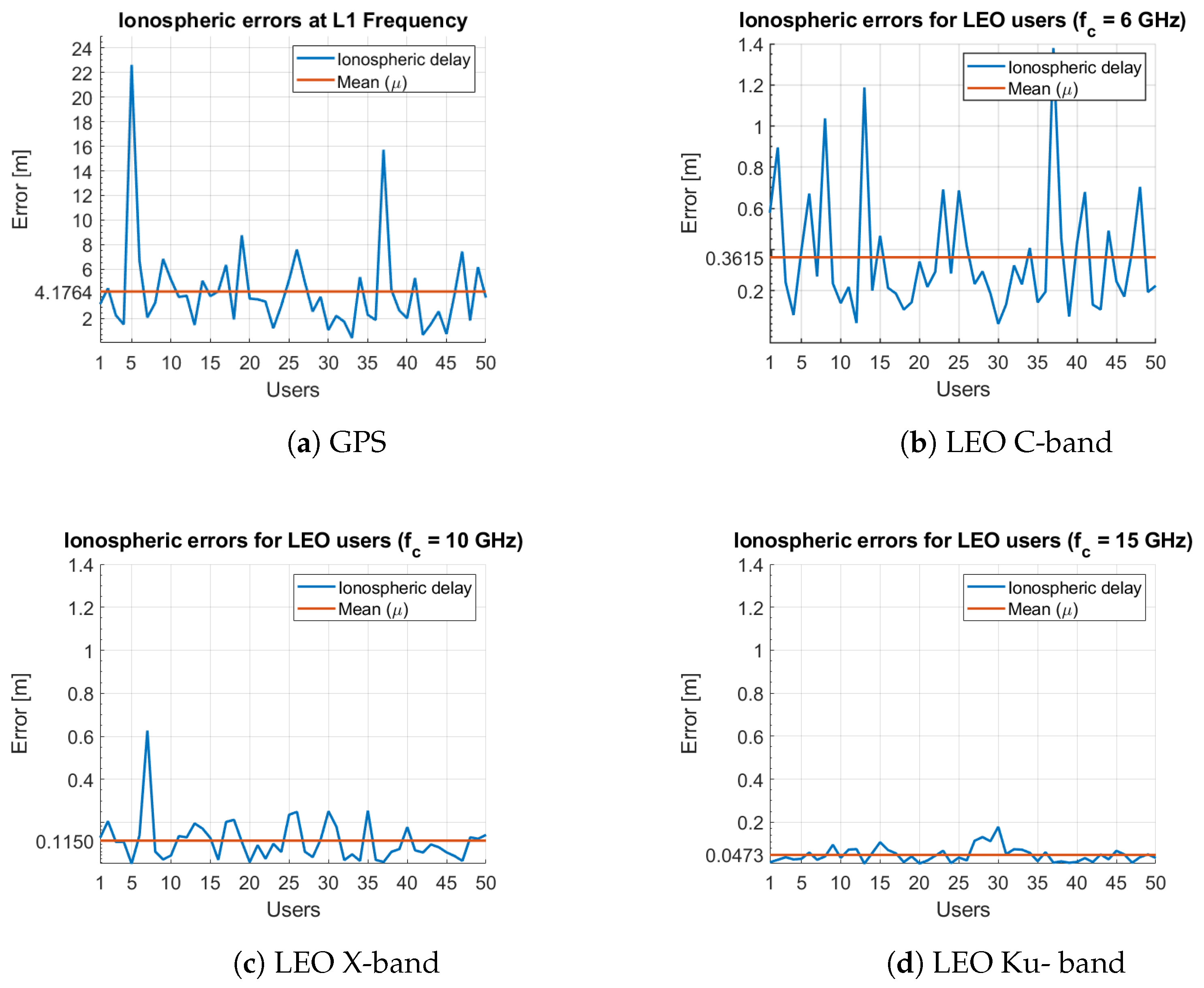
To analyze the effects of the ionospheric delay on LEO satellites, we ran four simulations using the IAMM model for 50 different users at random locations, dates, and times. We remark that the IAMM model does not depend on the satellite’s orbital height. However, we will observe how the frequencies of different satellite constellations influence the ionospheric delay.
The first run (Figure 8a) shows the ionospheric delay for users receiving signals from GPS satellites having an frequency. The second through fourth runs (Figure 8b–d) show the ionospheric delay for users receiving signals from LEO satellites having C-band, X-band, and Ku-band frequencies, respectively. It is worth noting that the figure corresponding to GPS has a different scale than the LEO figures.
The mean ionospheric delay decreased by , respectively, for C-band, X-band, and Ku-band frequencies compared to the GPS frequency. It is clear that the ionospheric delay for LEO satellites is significantly less than that of GPS satellites. This finding is based on a simple extension of the IAMM model to LEO-PNT, which was supported by the fact that IAMM is a generic and correction-independent model, which, once it is generated, remains valid indefinitely. Nevertheless, as the discussion in the next section shows, there are still several open challenges to be considered when extending a GNSS ionospheric model to LEO-PNT applications.
5. Discussion and Future Works
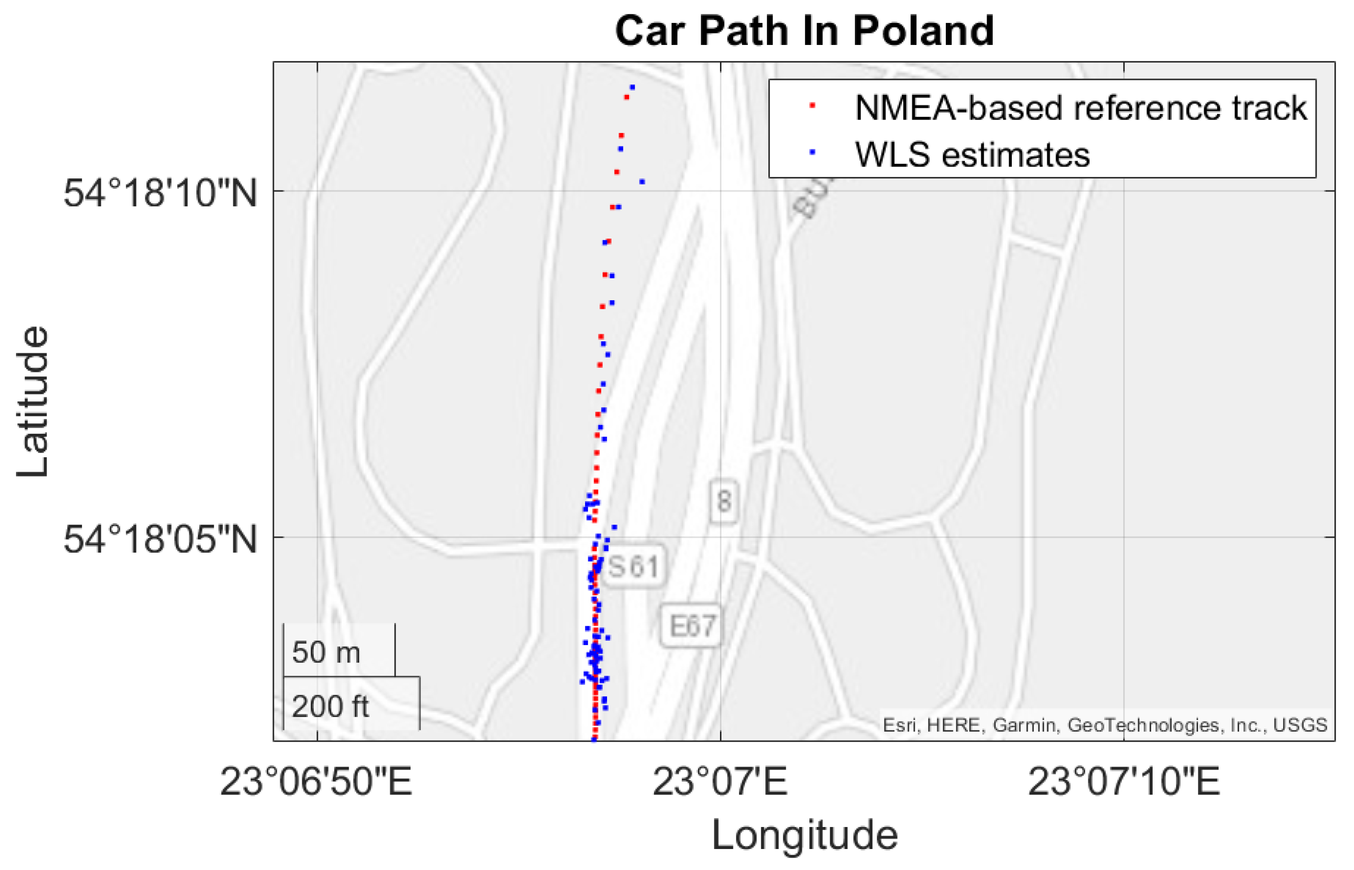
The results presented in the previous section showed that our proposed model (IAMM) accurately predicts the ionospheric delay for a given time and location and can even outperform the IRI and Klobuchar models when comparing the positioning errors of GNSS reference stations. However, the Klobuchar model showed the best performance for Android smartphones. As previously discussed, one possible explanation could be that a GNSS station’s exact position is calculated thoroughly, with high precision, before it is used as a reference to calculate the positioning error. In contrast, a smartphone’s exact position (used as a reference) is based on its NMEA estimates. Although these estimates are close to the actual position, they are still prone to errors. For example, in the data collected while driving on a highway in Poland, shown in Figure 7, the NMEA estimates showed that the phone’s position was outside of the road (white line) for a while, and the positioning errors of the WLS estimates made by IAMM were being calculated as a reference to the NMEA estimates. This proves we cannot entirely rely on Android data to validate our model. Future research will also focus on acquiring higher-accuracy reference tracks in dynamic conditions, using, for example, differential GNSS with the TAU GNSS roof antenna as a reference and a professional mobile GNSS receiver in a backpack to acquire more accurate reference data.
The results for LEO simulations showed a significant decrease in ionospheric delay for higher carrier frequencies. Fortunately, such higher frequencies are expected to be more present for LEO satellites, as they are preferred for communication services, which will be the prime usage of LEO satellites in the future. These higher frequencies will reduce the impact of the ionospheric delay (Equation (6)). On the other hand, lower frequencies from the L-bands are used for GNSS systems, resulting in a higher value for the ionospheric delay. Moreover, unlike GNSS, LEO satellites operate within the ionosphere (Figure 1), so their signals are affected only by the bottomside ionosphere, defined as the region below the F2 peak layer (hmF2). We can deduce from this unique distinction that LEO signals are not affected by the ionosphere as much as GNSS signals.
To enhance the accuracy of the IAMM, future research should focus on including anomalous data, such as ionospheric parameters under extreme space weather scenarios, to improve the robustness and responsiveness of the model. Moreover, to improve the quality of the positioning solution, the user’s environment should be considered; for example, one should look at whether the user is in an urban area (or an area with low signal quality) or an area with strong signal quality, and this remains a topic of future investigations. Future research should also work on finding and applying better mapping functions to scale the generated STEC value to suit the orbital height of the desired satellite. The scale factor should depend on the difference between the bottomside and topside ionosphere with respect to the time of day and day of year. The IAMM model can also be improved by applying compression algorithms to reduce the size of the Y matrix, making it easier to store in the memory of any device. Further improvements will also investigate more accurate modelling of the bottomside ionosphere, which is more relevant in LEO cases than the topside.
Overall, these steps should enhance the precision of the TEC estimation from an LEO satellite to a ground receiver and provide a more detailed description of the ionospheric behaviour for LEO satellite communications.
6. Conclusions
In this paper, we presented a detailed discussion of various state-of-the-art ionospheric models. Additionally, we introduced IAMM, a new ionospheric model based on interpolation from averaged data collected over 11 years. Our analysis indicates that the model we have developed exhibits a high level of accuracy in correcting errors caused by the ionosphere, especially in static conditions. The results obtained from our experiments clearly show that the model can effectively identify and rectify these errors, resulting in a significantly improved performance compared with traditional IRI and Klobuchar models in static receivers and a more moderate improvement in some of the tested dynamic scenarios. In addition to improving the positioning accuracy, our IAMM model has an advantage in relying solely on the matrix as a fixed input, making it a generic model that can work offline. This matrix can be conveniently stored in a device’s memory, making it easily accessible, especially for real-time applications. Another essential feature of the model is that it does not require atmospheric or any other external parameters to be available periodically, making it particularly useful for ionospheric studies on satellites that do not broadcast special parameters for ionospheric mitigation, which is the case for most of the LEO satellites in operation today.
Author Contributions
Conceptualization, M.I. and E.S.L.; methodology, M.I. and E.S.L.; software, M.I., A.G. and X.Z.; validation, M.I.; formal analysis, M.I. and E.S.L.; investigation, M.I., X.Z. and E.S.L.; writing—original draft preparation, M.I.; writing—review and editing, A.G., X.Z. and J.N. and E.S.L.; visualization, M.I.; supervision, J.N. and E.S.L.; project administration, J.N. and E.S.L.; funding acquisition, J.N. and E.S.L. All authors have read and agreed to the published version of the manuscript.
Funding
This research was funded by the INdoor navigation from CUBesAT Technology (INCUBATE) project under a grant from the Technology Industries of Finland Centennial Foundation and the Jane and Aatos Erkko Foundation (JAES), by the LEDSOL project funded within the LEAP-RE programme by the European Union’s Horizon 2020 Research and Innovation Program under Grant Agreement 963530 and the Academy of Finland grant agreement 352364, and by the APROPOS project funded within the Horizon 2020 Marie Skłodowska-Curie program grant agreement 956090.
Data Availability Statement
The data are available at: https://zenodo.org/records/10058636, DOI 10.5281/zenodo.10058635 (accessed on 10 December 2023).
Conflicts of Interest
The authors declare no conflicts of interest.
Correction Statement
This article has been republished with a minor correction to resolve spelling and grammatical errors. This change does not affect the scientific content of the article.
Abbreviations
The following abbreviations are used in this manuscript:
| AWGN | Additive white Gaussian noise |
| BDGIM | BeiDou Global Broadcast Ionospheric Delay Correction Model |
| CDDIS | Crustal Dynamics Data Information System |
| CMEs | Coronal mass ejections |
| COSPAR | Committee on Space Research |
| DFRs | Dual-frequency receivers |
| ED | Electron density |
| FFT | Fast Fourier transform |
| GEO | Geo-stationary orbit |
| GIMs | Global ionospheric maps |
| GNSS | Global Navigation Satellite Systems |
| GPS | Global Positioning System |
| IAMM | Interpolated and Averaged Memory Model |
| ID | Ionopsheric delay |
| IGS | International GNSS Service |
| IONEX | IONosphere map EXchange format |
| IoT | Internet of Things |
| IRI | International Reference Ionosphere |
| ISR | Incoherent scattered radar |
| IWG | Ionosphere Working Group |
| LEO | Low Earth orbit |
| LOS | Line of sight |
| MEO | Medium Earth orbit |
| ML | Machine learning |
| NASA | National Aeronautics and Space Administration |
| NLOS | Non-line-of-sight |
| NLS | National Land Survey of Finland |
| NMEA | National Marine Electronics Association |
| NOAA | National Oceanic and Atmospheric Administration |
| PNT | Position, Navigation, and Timing |
| PPP | Precise point positioning |
| QZSS | Quasi-Zenith Satellite System |
| Q4DIM | Quasi-4-Dimension Ionospheric Modeling |
| RF | Radio frequency |
| RIM | Regional ionospheric map |
| RINEX | Receiver-independent exchange format |
| RMS | Root mean square |
| RSS | Received signal strength |
| RT-GIMs | Real-time global ionospheric maps |
| SLM-MF | Single-layer model mapping function |
| SFRs | Single-frequency receivers |
| SPP | Single-point positioning |
| STEC | Slant total electron content |
| TDL | Tapped delay line |
| TEC | Total electron content |
| TECU | TEC units |
| ToA | Time of arrival |
| URSI | Union of Radio Science |
| VTEC | Vertical total electron content |
| WLS | Weighted least squares |
References
- Reid, T.G.; Neish, A.M.; Walter, T.; Enge, P.K. Broadband LEO Constellations for Navigation. Navigation 2018, 65, 205–220. [Google Scholar] [CrossRef]
- Shi, C.; Zhang, Y.; Li, Z. Revisiting Doppler positioning performance with LEO satellites. GPS Solut. 2023, 27, 126. [Google Scholar] [CrossRef]
- Kassas, Z.Z.M. Navigation from Low-Earth Orbit. In Position, Navigation, and Timing Technologies in the 21st Century; John Wiley & Sons, Ltd.: Hoboken, NJ, USA, 2020; Chapter 43; pp. 1381–1412. [Google Scholar] [CrossRef]
- Prol, F.S.; Ferre, R.M.; Saleem, Z.; Välisuo, P.; Pinell, C.; Lohan, E.S.; Elsanhoury, M.; Elmusrati, M.; Islam, S.; Çelikbilek, K.; et al. Position, Navigation, and Timing (PNT) Through Low Earth Orbit (LEO) Satellites: A Survey on Current Status, Challenges, and Opportunities. IEEE Access 2022, 10, 83971–84002. [Google Scholar] [CrossRef]
- Morales-Ferre, R.; Lohan, E.S.; Falco, G.; Falletti, E. GDOP-based analysis of suitability of LEO constellations for future satellite-based positioning. In Proceedings of the 2020 IEEE International Conference on Wireless for Space and Extreme Environments (WiSEE), Virtual, 12–14 October 2020. [Google Scholar]
- Johnston, G.; Riddell, A.; Hausler, G. The International GNSS Service. In Springer Handbook of Global Navigation Satellite Systems; Springer International Publishing: Cham, Switzerland, 2017; pp. 967–982. [Google Scholar] [CrossRef]
- Teunissen, P.; Montenbruck, O. Springer Handbook of Global Navigation Satellite Systems, 1st ed.; Springer Handbooks; Springer International Publishing: Cham, Switzerland, 2017. [Google Scholar]
- Morales-Ferre, R.; Richter, P.; Falletti, E.; de la Fuente, A.; Lohan, E.S. A Survey on Coping With Intentional Interference in Satellite Navigation for Manned and Unmanned Aircraft. IEEE Commun. Surv. Tutorials 2020, 22, 249–291. [Google Scholar] [CrossRef]
- Menzione, F.; Paonni, M. LEO-PNT Mega-Constellations: A New Design Driver for the Next Generation MEO GNSS Space Service Volume and Spaceborne Receivers. In Proceedings of the 2023 IEEE/ION Position, Location and Navigation Symposium (PLANS), Monterey, CA, USA, 24–27 April 2023; pp. 1196–1207. [Google Scholar] [CrossRef]
- Gutierrez, P. ESA LEO PNT Program Getting Underway. Inside GNSS Journal. 2023. Available online: https://insidegnss.com/esa-leo-pnt-program-getting-underway/ (accessed on 10 December 2023).
- Industry Invited to Bid for Ow-Earth Orbit Satnav Demo. Newsletters. Available online: https://www.esa.int/Applications/Navigation/Industry_invited_to_bid_for_low-Earth_orbit_satnav_demo (accessed on 10 December 2023).
- Janssen, T.; Koppert, A.; Berkvens, R.; Weyn, M. A Survey on IoT Positioning Leveraging LPWAN, GNSS, and LEO-PNT. IEEE Internet Things J. 2023, 10, 11135–11159. [Google Scholar] [CrossRef]
- PNT from and for Space: What Are the Steps Necessary to Make LEO Positioning a Eality? Novatel Webinar. 2023. Available online: https://novatel.com/tech-talk/webinars/pnt-from-and-for-space-leo-positioning (accessed on 10 December 2023).
- Joerger, M.; Gratton, L.; Pervan, B.; Cohen, C.E. Analysis of Iridium-Augmented GPS for Floating Carrier Phase Positioning. Navigation 2010, 57, 137–160. [Google Scholar] [CrossRef]
- Su, M.; Su, X.; Zhao, Q.; Liu, J. BeiDou Augmented Navigation from Low Earth Orbit Satellites. Sensors 2019, 19, 198. [Google Scholar] [CrossRef]
- Guan, M.; Xu, T.; Gao, F.; Nie, W.; Yang, H. Optimal Walker Constellation Design of LEO-Based Global Navigation and Augmentation System. Remote Sens. 2020, 12, 1845. [Google Scholar] [CrossRef]
- Li, T.; Wang, L.; Fu, W.; Han, Y.; Zhou, H.; Chen, R. Bottomside ionospheric snapshot modeling using the LEO navigation augmentation signal from the Luojia-1A satellite. GPS Solut. 2022, 26, 6. [Google Scholar] [CrossRef]
- Sedeek, A. Ionosphere delay remote sensing during geomagnetic storms over Egypt using GPS phase observations. Arab. J. Geosci. 2020, 13, 811. [Google Scholar] [CrossRef]
- Goodman, J.M. Space Weather Telecommunications; Springer Science & Business Media: Cham, Switzerland, 2005. [Google Scholar] [CrossRef]
- Bilitza, D.; Altadill, D.; Zhang, Y.; Mertens, C.; Truhlik, V.; Richards, P.; McKinnell, L.A.; Reinisch, B. The International Reference Ionosphere 2012—A model of international collaboration. J. Space Weather Space Clim. 2014, 4, A07. [Google Scholar] [CrossRef]
- Davies, K. Ionospheric Radio Propagation. 1965. Available online: https://digital.library.unt.edu/ark:/67531/metadc13264/ (accessed on 10 December 2023).
- Jakowski, N.; Mayer, C.; Hoque, M.M.; Wilken, V. Total electron content models and their use in ionosphere monitoring. Radio Sci. 2011, 46, RS0D18. [Google Scholar] [CrossRef]
- Yasyukevich, Y.V.; Zatolokin, D.; Padokhin, A.; Wang, N.; Nava, B.; Li, Z.; Yuan, Y.; Yasyukevich, A.; Chen, C.; Vesnin, A. Klobuchar, NeQuickG, BDGIM, GLONASS, IRI-2016, IRI-2012, IRI-Plas, NeQuick2, and GEMTEC Ionospheric Models: A Comparison in Total Electron Content and Positioning Domains. Sensors 2023, 23, 4773. [Google Scholar] [CrossRef] [PubMed]
- Kaplan, E.D.; Hegarty, C.J. Understanding GPS, Principles and Applications, 3rd ed.; Artech House: London, UK, 2017. [Google Scholar]
- Grunwald, G.; Ciećko, A.; Kozakiewicz, T.; Krasuski, K. Analysis of GPS/EGNOS Positioning Quality Using Different Ionospheric Models in UAV Navigation. Sensors 2023, 23, 1112. [Google Scholar] [CrossRef] [PubMed]
- Panda, S.K.; Haralambous, H.; Kavutarapu, V. Global Longitudinal Behavior of IRI Bottomside Profile Parameters From FORMOSAT-3/COSMIC Ionospheric Occultations. J. Geophys. Res. Space Phys. 2018, 123, 7011–7028. [Google Scholar] [CrossRef]
- Smirnov, A.; Shprits, Y.; Prol, F.; Lühr, H.; Berrendorf, M.; Zhelavskaya, I.; Xiong, C. A novel neural network model of Earth’s topside ionosphere. Sci. Rep. 2023, 13, 1303. [Google Scholar] [CrossRef] [PubMed]
- Lei, J.; Zhu, Q.; Wang, W.; Burns, A.G.; Zhao, B.; Luan, X.; Zhong, J.; Dou, X. Response of the topside and bottomside ionosphere at low and middle latitudes to the October 2003 superstorms. J. Geophys. Res. Space Phys. 2015, 120, 6974–6986. [Google Scholar] [CrossRef]
- Jarmołowski, W.; Ren, X.; Wielgosz, P.; Krypiak-Gregorczyk, A. On the advantage of stochastic methods in the modeling of ionospheric total electron content: Southeast Asia case study. Meas. Sci. Technol. 2019, 30, 044008. [Google Scholar] [CrossRef]
- Alizadeh, M.M.; Schuh, H.; Schmidt, M. Ray tracing technique for global 3-D modeling of ionospheric electron density using GNSS measurements. Radio Sci. 2015, 50, 539–553. [Google Scholar] [CrossRef]
- Natras, R.; Goss, A.; Halilovic, D.; Magnet, N.; Mulic, M.; Schmidt, M.; Weber, R. Regional Ionosphere Delay Models Based on CORS Data and Machine Learning. Navig. J. Inst. Navig. 2023, 70, navi.577. [Google Scholar] [CrossRef]
- Farzaneh, S.; Forootan, E. Reconstructing Regional Ionospheric Electron Density: A Combined Spherical Slepian Function and Empirical Orthogonal Function Approach. Surv. Geophys. 2017, 39, 289–309. [Google Scholar] [CrossRef]
- Zhu, F.; Zhi, N.; Fu, H. A Data-Driven Forecast Model of Ionospheric Slant Total Electron Content Based on Decision Trees. In Proceedings of the 2023 International Applied Computational Electromagnetics Society Symposium (ACES), Monterey/Seaside, CA, USA, 26–30 March 2023. [Google Scholar] [CrossRef]
- Massarweh, L.; Fortunato, M.; Gioia, C. Assessment of Real-time Multipath Detection with Android Raw GNSS Measurements by Using a Xiaomi Mi 8 Smartphone. In Proceedings of the 2020 IEEE/ION Position, Location and Navigation Symposium (PLANS), Portland, OR, USA, 20–23 April 2020; pp. 1111–1122. [Google Scholar] [CrossRef]
- Lohan, E.S.; Bierwirth, K.; Kodom, T.; Ganciu, M.; Lebik, H.; Elhadi, R.; Cramariuc, O.; Mocanu, I. Standalone Solutions for Clean and Sustainable Water Access in Africa Through Smart UV/LED Disinfection, Solar Energy Utilization, and Wireless Positioning Support. IEEE Access 2023, 11, 81882–81899. [Google Scholar] [CrossRef]
- Lohan, E.S.; Kodom, T.; Lebik, H.; Grenier, A.; Zhang, X.; Cramariuc, O.; Mocanu, I.; Bierwirth, K.; Nurmi, J. Raw GNSS Data Analysis for the LEDSOL Project—Preliminary Results and Way Ahead. In Proceedings of the WiP in Hardware and Software for Location Computation (WIPHAL 2023), Castellon, Spain, 6–8 June 2023; 3434. [Google Scholar]
- Hamza, V.; Stopar, B.; Sterle, O.; Pavlovčič-Prešeren, P. Low-Cost Dual-Frequency GNSS Receivers and Antennas for Surveying in Urban Areas. Sensors 2023, 23, 2861. [Google Scholar] [CrossRef] [PubMed]
- Liu, Q.; Gao, C.; Peng, Z.; Zhang, R.; Shang, R. Smartphone Positioning and Accuracy Analysis Based on Real-Time Regional Ionospheric Correction Model. Sensors 2021, 21, 3879. [Google Scholar] [CrossRef] [PubMed]
- Panda a, S.K.; Harikaa, B.; Vineetha, P.; Kumar Dabbakutib, J.R.K.; Akhila, S.; Srujanaa, G. Validity of Different Global Ionospheric TEC Maps over Indian Region. In Proceedings of the 2021 3rd International Conference on Advances in Computing, Communication Control and Networking (ICAC3N), Greater Noida, India, 17–18 December 2021; pp. 1749–1755. [Google Scholar] [CrossRef]
- Klobuchar, J. Ionospheric Time-Delay Algorithm for Single-Frequency GPS Users. IEEE Trans. Aerosp. Electron. Syst. 1987, AES-23, 325–331. [Google Scholar] [CrossRef]
- Mäkelä, M.K.K. Comparison and Development of Ionospheric Correction Methods in GNSS. Master’s Thesis, Tampere University, Tampere, Finland, 2016. Available online: https://trepo.tuni.fi/handle/123456789/24484 (accessed on 10 December 2023).
- European GNSS Open Service. Ionospheric Correction Algorithm for Galileo Single Frequency Users. 2016. Available online: https://www.gsc-europa.eu/sites/default/files/sites/all/files/Galileo_Ionospheric_Model.pdf (accessed on 30 October 2023).
- Sanz Subirana, J.; Juan Zornoza, J.M.; Hernández-Pajares, M. NeQuick Ionospheric Model—Navipedia. 2017. Available online: https://gssc.esa.int/navipedia/index.php?title=NeQuick_Ionospheric_Model (accessed on 13 October 2023).
- Mallika, I.L.; Ratnam, D.V.; Ostuka, Y.; Sivavaraprasad, G.; Raman, S. Implementation of Hybrid Ionospheric TEC Forecasting Algorithm Using PCA-NN Method. IEEE J. Sel. Top. Appl. Earth Obs. Remote Sens. 2019, 12, 371–381. [Google Scholar] [CrossRef]
- Boisits, J.; Glaner, M.; Weber, R. Regiomontan: A Regional High Precision Ionosphere Delay Model and Its Application in Precise Point Positioning. Sensors 2020, 20, 2845. [Google Scholar] [CrossRef] [PubMed]
- Froń, A.; Galkin, I.; Krankowski, A.; Bilitza, D.; Hernández-Pajares, M.; Reinisch, B.; Li, Z.; Kotulak, K.; Zakharenkova, I.; Cherniak, I.; et al. Towards Cooperative Global Mapping of the Ionosphere: Fusion Feasibility for IGS and IRI with Global Climate VTEC Maps. Remote Sens. 2020, 12, 3531. [Google Scholar] [CrossRef]
- Liu, Q.; Hernández-Pajares, M.; Yang, H.; Monte-Moreno, E.; Roma-Dollase, D.; García-Rigo, A.; Li, Z.; Wang, N.; Laurichesse, D.; Blot, A.; et al. The cooperative IGS RT-GIMs: A reliable estimation of the global ionospheric electron content distribution in real time. Earth Syst. Sci. Data 2021, 13, 4567–4582. [Google Scholar] [CrossRef]
- Schaer, S.; Gurtner, W.; Feltens, J. IONEX: The IONosphere Map EXchange Format Version 1.1. 1998. Available online: https://www.aiub.unibe.ch/download/ionex/ionex1.pdf (accessed on 10 December 2023).
- Kim, J.; Kim, M. Determination of Ionospheric Delay Scale Factor for Low Earth Orbit using the International Reference Ionosphere Model. Korean J. Remote Sens. 2014, 30, 331–339. [Google Scholar] [CrossRef]
- Kim, J.; Kim, M. NeQuick G model based scale factor determination for using SBAS ionosphere corrections at low earth orbit. Adv. Space Res. 2020, 65, 1414–1423. [Google Scholar] [CrossRef]
- Li, S.Y.; Liu, C. Modeling the effects of ionospheric scintillations on LEO Satellite communications. IEEE Commun. Lett. 2004, 8, 147–149. [Google Scholar] [CrossRef]
- Bilitza, D.; Pezzopane, M.; Truhlik, V.; Altadill, D.; Reinisch, B.W.; Pignalberi, A. The International Reference Ionosphere Model: A Review and Description of an Ionospheric Benchmark. Rev. Geophys. 2022, 60, e2022RG000792. [Google Scholar] [CrossRef]
- Jin, X.; Song, S. Near real-time global ionospheric total electron content modeling and nowcasting based on GNSS observations. J. Geod. 2023, 97, 27. [Google Scholar] [CrossRef]
- Maria, A. Introduction To Modeling and Simulation. In Proceedings of the Winter Simulation Conference Proceedings, Atlanta, GA, USA, 7–10 December 1997; pp. 7–13. [Google Scholar] [CrossRef]
- Hernández-Pajares, M.; Juan, J.M.; Sanz, J.; Orus, R.; Garcia-Rigo, A.; Feltens, J.; Komjathy, A.; Schaer, S.C.; Krankowski, A. The IGS VTEC maps: A reliable source of ionospheric information since 1998. J. Geod. 2009, 83, 263–275. [Google Scholar] [CrossRef]
- Li, W.; Chen, Y. Establishment of polynomial regional ionospheric delay model by using GNSS dual-frequency combined observations. J. Phys. Conf. Ser. 2020, 1550, 042057. [Google Scholar] [CrossRef]
- Marshall, J.; Plumb, R.A. Introduction to Ionospheric Physics; International Geophysics Series; Academic Press: Cambridge, MA, USA, 1969. [Google Scholar]
- Solar and Geophysical Event Reports. National Oceanic and Atmospheric Administration (NOAA), Space Weather Prediction Center. 2023. Available online: ftp://ftp.swpc.noaa.gov/pub/indices/events/20230805events.txt (accessed on 10 December 2023).
- Grenier, A. Development of a GNSS Positioning Application under Android OS Using GALILEO Signals. Master’s Thesis, Ecole Nationale de Sciences Geographiques, Champs-sur-Marne, France, 2019. [Google Scholar]
Figure 1.
Ionosphere layer representation w.r.t. to satellite altitudes.

Figure 2.
Illustration of IONEX file content.

Figure 3.
Illustration of VTEC and STEC corresponding to a satellite signal.

Figure 4.
The process of collecting and organizing data from IONEX files.

Figure 5.
Example for VTEC calculation using IAMM for User A located at Tampere University.

Figure 6.
A snapshot world TEC map as predicted by the two models for 5 August 2023 at 22:00 UTC. (a) Data from our IAMM model. (b) Data from IGS.
Figure 6.
A snapshot world TEC map as predicted by the two models for 5 August 2023 at 22:00 UTC. (a) Data from our IAMM model. (b) Data from IGS.

Figure 7.
Map of the car path predicted by NMEA and WLS estimates.

Figure 8.
Ionospheric delays for GPS and LEO users at random times and locations. Note that the scale of the y-axis for plot (a) is different from that of the other three plots (b–d).
Figure 8.
Ionospheric delays for GPS and LEO users at random times and locations. Note that the scale of the y-axis for plot (a) is different from that of the other three plots (b–d).


Table 1.
Summary of ionospheric models reviewed (ED: electron density, ID: ionospheric delay, ISR: incoherent scatter radar).
Table 1.
Summary of ionospheric models reviewed (ED: electron density, ID: ionospheric delay, ISR: incoherent scatter radar).
| Ref. | Model | Type | Broadcast | Input Data | Direct Output Data |
|---|---|---|---|---|---|
| [40] | Klobuchar | Empirical | Yes | Atmospheric coef., approx. receiver position | ID |
| [42] | NeQuick | Empirical | Yes | Atmospheric coef., approx. user position | ED, ID |
| [31,33,44,45] | Neural networks | Data-driven | No | Data from other models/stations | TEC, ID |
| [52] | IRI | Empirical | No | Ionosondes, ISRs, in situ data (satellites) | ED, ID, ionosphere detailed composition (see Section 2.5) |
| [53] | IGS (GIMs) | Mathematical | No | Dual-frequency measurements from GNSS stations | IONEX files |
| This work | IAMM | Data-driven | No | Approx. receiver position, Y matrix (see Section 3.2) | TEC, ID |
Table 2.
Solar year mapping table.
| R | 0 | 1 | 2 | 3 | 4 | 5 | 6 | 7 | 8 | 9 | 10 |
| Solar Year | 5 | 6 | 7 | 8 | 9 | 10 | 11 | 1 | 2 | 3 | 4 |
Table 3.
Correlation coefficients between TEC values generated by IAMM and IGS.
| Number of Points Used in Statistics | Correlation Coefficient |
|---|---|
| 5183 | 0.9283 |
| 15,549 | 0.9574 |
| 31,098 | 0.9589 |
Table 4.
3D positioning errors from GNSS receivers using different ionospheric correction models.
| AVG [m] | No Correction | Klobuchar | IRI | IAMM (Proposed) |
|---|---|---|---|---|
| Mean | 5.390 | 3.244 | 3.159 | 1.976 |
| – | (−39.7%) | (−41.4%) | (−63.3%) | |
| StD (1-) | 1.277 | 1.051 | 1.0682 | 0.848 |
| – | (−17.7%) | (−16.4%) | (−33.6%) | |
| a Using observations from Tampere University (high-grade) | ||||
| AVG [m] | No Correction | Klobuchar | IRI | IAMM (Proposed) |
| Mean | 6.209 | 4.252 | 4.397 | 4.1708 |
| – | (−31.5%) | (−29.2%) | (−32.8%) | |
| StD (1-) | 3.470 | 3.219 | 3.141 | 3.164 |
| – | (−7.2%) | (−9.5%) | (−8.8%) | |
| b Using observations from the FinnRef network (high-grade) | ||||
| AVG [m] | No Correction | Klobuchar | IRI | IAMM (Proposed) |
| Mean | 42.815 | 34.052 | 38.884 | 36.388 |
| – | (−20.5%) | (−9.2%) | (−15%) | |
| StD (1-) | 18.710 | 18.103 | 18.397 | 18.211 |
| – | (−3.2%) | (−1.7%) | (−2.7%) | |
| c Using observations from Android smartphones (low-power) | ||||
Disclaimer/Publisher’s Note: The statements, opinions and data contained in all publications are solely those of the individual author(s) and contributor(s) and not of MDPI and/or the editor(s). MDPI and/or the editor(s) disclaim responsibility for any injury to people or property resulting from any ideas, methods, instructions or products referred to in the content. |
© 2023 by the authors. Licensee MDPI, Basel, Switzerland. This article is an open access article distributed under the terms and conditions of the Creative Commons Attribution (CC BY) license (https://creativecommons.org/licenses/by/4.0/).
Share and Cite
MDPI and ACS Style
Imad, M.; Grenier, A.; Zhang, X.; Nurmi, J.; Lohan, E.S. Ionospheric Error Models for Satellite-Based Navigation—Paving the Road towards LEO-PNT Solutions. Computers 2024, 13, 4. https://doi.org/10.3390/computers13010004
AMA Style
Imad M, Grenier A, Zhang X, Nurmi J, Lohan ES. Ionospheric Error Models for Satellite-Based Navigation—Paving the Road towards LEO-PNT Solutions. Computers. 2024; 13(1):4. https://doi.org/10.3390/computers13010004
Chicago/Turabian StyleImad, Majed, Antoine Grenier, Xiaolong Zhang, Jari Nurmi, and Elena Simona Lohan. 2024. "Ionospheric Error Models for Satellite-Based Navigation—Paving the Road towards LEO-PNT Solutions" Computers 13, no. 1: 4. https://doi.org/10.3390/computers13010004
Note that from the first issue of 2016, this journal uses article numbers instead of page numbers. See further details here.