
Requirement Change Prediction Model for Small Software Systems
by
 , , and
Rida Fatima
1, 
Furkh Zeshan
1,
Adnan Ahmad
1,
Muhamamd Hamid
2,
Imen Filali
3,*,
Amel Ali Alhussan
3 and
Hanaa A. Abdallah
4 1
Department of Computer Science, COMSATS University Islamabad, Lahore Campus, Lahore 54000, Pakistan
2
Department of Computer Science, Government College Women University, Sialkot 51310, Pakistan
3
Department of Computer Sciences, College of Computer and Information Sciences, Princess Nourah Bint Abdulrahman University, P.O. Box 84428, Riyadh 11671, Saudi Arabia
4
Department of Information Technology, College of Computer and Information Sciences, Princess Nourah Bint Abdulrahman University, P.O. Box 84428, Riyadh 84428, Saudi Arabia
*
Author to whom correspondence should be addressed.
Computers 2023, 12(8), 164; https://doi.org/10.3390/computers12080164
Submission received: 10 July 2023
/
Revised: 1 August 2023
/
Accepted: 10 August 2023
/
Published: 14 August 2023
(This article belongs to the Special Issue Best Practices, Challenges and Opportunities in Software Engineering)
Abstract
:The software industry plays a vital role in driving technological advancements. Software projects are complex and consist of many components, so change is unavoidable in these projects. The change in software requirements must be predicted early to preserve resources, since it can lead to project failures. This work focuses on small-scale software systems in which requirements are changed gradually. The work provides a probabilistic prediction model, which predicts the probability of changes in software requirement specifications. The first part of the work considers analyzing the changes in software requirements due to certain variables with the help of stakeholders, developers, and experts by the questionnaire method. Then, the proposed model incorporates their knowledge in the Bayesian network as conditional probabilities of independent and dependent variables. The proposed approach utilizes the variable elimination method to obtain the posterior probability of the revisions in the software requirement document. The model was evaluated by sensitivity analysis and comparison methods. For a given dataset, the proposed model computed the low state revisions probability to 0.42, and the high state revisions probability to 0.45. Thus, the results proved that the proposed approach can predict the change in the requirements document accurately by outperforming existing models.
1. Introduction
The software industry plays a significant role in improving human life, ranging from businesses, communication, entertainment, education, and a lot more. Software is an integral part of devices, applications, and systems on which people rely for various daily tasks [1]. Besides their numerous benefits, faulty software applications also have negative effects on human life; for example, in the case of a fault in a safety critical system, software can create life-threatening situations. Similarly, in the case of business applications, software faults can derail software productivity or operations resulting in an increased cost and time. To cater to these conditions, the software industry encompasses various activities, during software development, testing, deployment, maintenance, and support. As a result of these activities, software is becoming technologically advanced, struggling to address the ever-expanding business requirements, along with the preferences of various stakeholders [2]. Similarly, software engineers also face challenges in adapting to new circumstances [3]. In order to quantify the efforts of a change in software under development, a few works have been proposed for small-scale software systems [4,5]. Small-scale software systems have attracted much attention recently because most of the small software companies do not have properly defined procedures to face these challenges, which leads to failures. As the software requirements can change at any phase of the software development because of a change in stakeholder needs resulting in an increased cost, tightening of the schedule, and issues of scalability [6]. Therefore, there is a need to predict the change in software requirements at the early stages of development. Studies have illustrated that an error occurring in the development phase takes approximately 8 h to be resolved, whereas if it occurs in the requirement phase, it might take only 15 min to be resolved [7,8]. In software development, requirement gathering is the first step, where artificial intelligence (AI) tools, along with expert judgment, can be used to predict changes in software requirements [9]. In this regard, researchers have focused on how to also incorporate human experience into AI to predict change accurately [9,10]. Currently, most prediction models only utilize expert knowledge and consider a limited set of software metrics that represent different aspects of software, such as ambiguity, coupling, completeness, etc., to develop change prediction models [10]. The core requirement metrics with the knowledge of all the domain experts, including stakeholders and developers, are included in the prediction models. In this case, the probability of software requirement changes can be decreased, and the results can be improved [11]. The stakeholders describe the user requirements, use cases, and events; thus, they can have a vital role in defining the system requirements functions and operations. Moreover, the developers could provide a detailed system design and implementation description [12]. In contrast, in the AI field which is based on classification, learning, and prediction, certain authors [11,12] have proposed models for the prediction of changes in requirements. In this regard, a probabilistic AI technique such as Bayesian probabilistic reasoning can be used that is closely related to software engineering.
This work proposes a probabilistic prediction model to predict the probability of changes in software requirement specifications. This work extends that of [13] by considering new features like specificity, requirement completeness, degree of revision, and degree of commitment, etc., by using a Bayesian network to predict changes in the requirement specification. The features have enhanced the effectiveness of the prediction of the proposed approach. The main contributions of the work are summarized as follows.
- -
- Performing a detailed literature review and deriving the requirement variables that support the prediction model for acquiring the probability of changes.
- -
- Defining the core requirement variables with the consultation of experts and weighting techniques.
- -
- Developing a refined dataset with the help of a questionnaire. This questionnaire was given to stakeholders, developers, and experts to acquire their knowledge of the set of requirements.
- -
- Developing a prediction model in the Bayesian network with nodes and arcs to predict the probability of changes in software requirements. Nodes are the core variables with the conditional probabilities acquired by the dataset.
- -
- The proposed algorithm includes a variable elimination method for predicting requirement changes in the specification document. This algorithm takes the Bayesian network conditional probabilities as an input and provides the probability of revisions in the requirement document.
- -
- Evaluation of the proposed model by comparing it with the existing models in terms of the accuracy and validity of this model.
2. Related Work
This section reviews the latest approaches in which requirement change prediction models are proposed.
According to the literature, Park et al. [14] mined the required attributes of a large software project that can be used to obtain the requirement-relevant faults. The authors conducted a survey indicating that ambiguous and faulty requirements cause relevant deficiencies. Hein et al. [15] proposed an automatic requirement prediction tool in which the part of speech elements of the requirements statement are given as inputs. These data are taken as relators to design relations between requirements.
Arora et al. [16] investigated the impact of changes in the requirements of natural language processing. The developed model used the requirements of natural language processing as inputs. The user then updates the requirement document after the system has identified the required statement phrases and calculated the token pairwise similarity scores. In an early stage of software development, the fault density was predicted by Yadav et al. [17] using fuzzy logic. Three software metrics were incorporated for each requirement design and development stage.
In the model described in [13], del Sagrado et al. merged the software engineering field into AI techniques. The developed model used expert knowledge to predict the requirement specification document. A Bayesian network named “requisites” was induced in a tool that predicts the degree of modifications of the requirement document. Zhang et al. [18] suggested an inference algorithm in Bayesian networks, which helps to trace the cause and impacts of the variables in the system. This is also supportive of making wise decisions in intelligent systems.
Literature studies lack a consideration of the sophisticated variables (e.g., developer skills, stakeholder expertise, technological needs, verification, consistency, ambiguity, and quality). These variables were collected from the literature by using weighting techniques and shortlisted using expert opinion. The experts categorized these variables into two groups: project estimation and management. Table 1 provides the details of the variables and their descriptions.
The project estimation variables are less well studied in the prediction methods as compared to the management group. There is a great need for an advanced prediction model that should include the knowledge of experts, developers, and stakeholders to predict the changes in requirement specifications and quantify their effects while including all necessary variables [19].

Table 1.
Core variables with descriptions.
| Group | Variables | Description |
|---|---|---|
| Project/Estimation Group | Ambiguity | Sometimes the requirements are not understandable and provide double meanings that may cause changes [20]. |
| Cost and schedule | Project cost is the money needed to complete the project [21]. The schedule is the time allocated by the project managers for managing requirements [22]. | |
| Specificity | Specificity deals with the meanings of the requirement. It demonstrates that all of the people have the same interpretation of the requirement statement [23]. | |
| Quality | Requirement changes affect the quality. It is necessary to ensure that the system’s quality meets the standards [24]. | |
| Technological needs | Sometimes the consideration of new technology for the software development may cause changes [25]. | |
| Consistency | It describes that the requirements are presented in a detailed way and serve the intended purpose [26]. | |
| Dependencies | It interprets the unexpected relationships between requirements. The requirement may depend on another variable not specified in the requirements document [27]. | |
| Reusability | It interprets whether the particular requirement can be reused. If it is reused from repository, then the number of repetitions will be counted [28]. | |
| Management Group | Completeness | It describes that the requirement carry comprehensive meanings, and no information is left behind [23]. |
| Commitment | It interprets that requirement needs further communication for acceptance [29]. | |
| Developer skills | Developer skills play an important role in the timely completion of software. If the developers are skilled, then when changes occur during the development phase, they can easily manage them [30]. | |
| Variability | Requirement changes are natural processes and can occur at any project phase. These are necessary to manage because it affects the complete development process, cost, schedule design, and implementation [31]. | |
| Verification | When requirement changes occur, it is necessary to verify whether these changes reflect the intended purpose or not [32]. | |
| Expert knowledge | After a requirement change, experts are needed to decide on how the changes will be integrated into the system [33]. | |
| SRS document revisions | The SRS document provides an overall description of the system, its purpose, revisions, and its requirement specifications [34]. | |
| Stakeholder expertise | Requirement changes frequently occur due to the incompetentency of stakeholders because they provide the system’s requirements [35]. |
In this work, a Bayesian network model is constructed by considering comprehensive variables (limitations of existing models) along with the algorithms to measure the probability of a change in requirements.
3. Proposed Approach
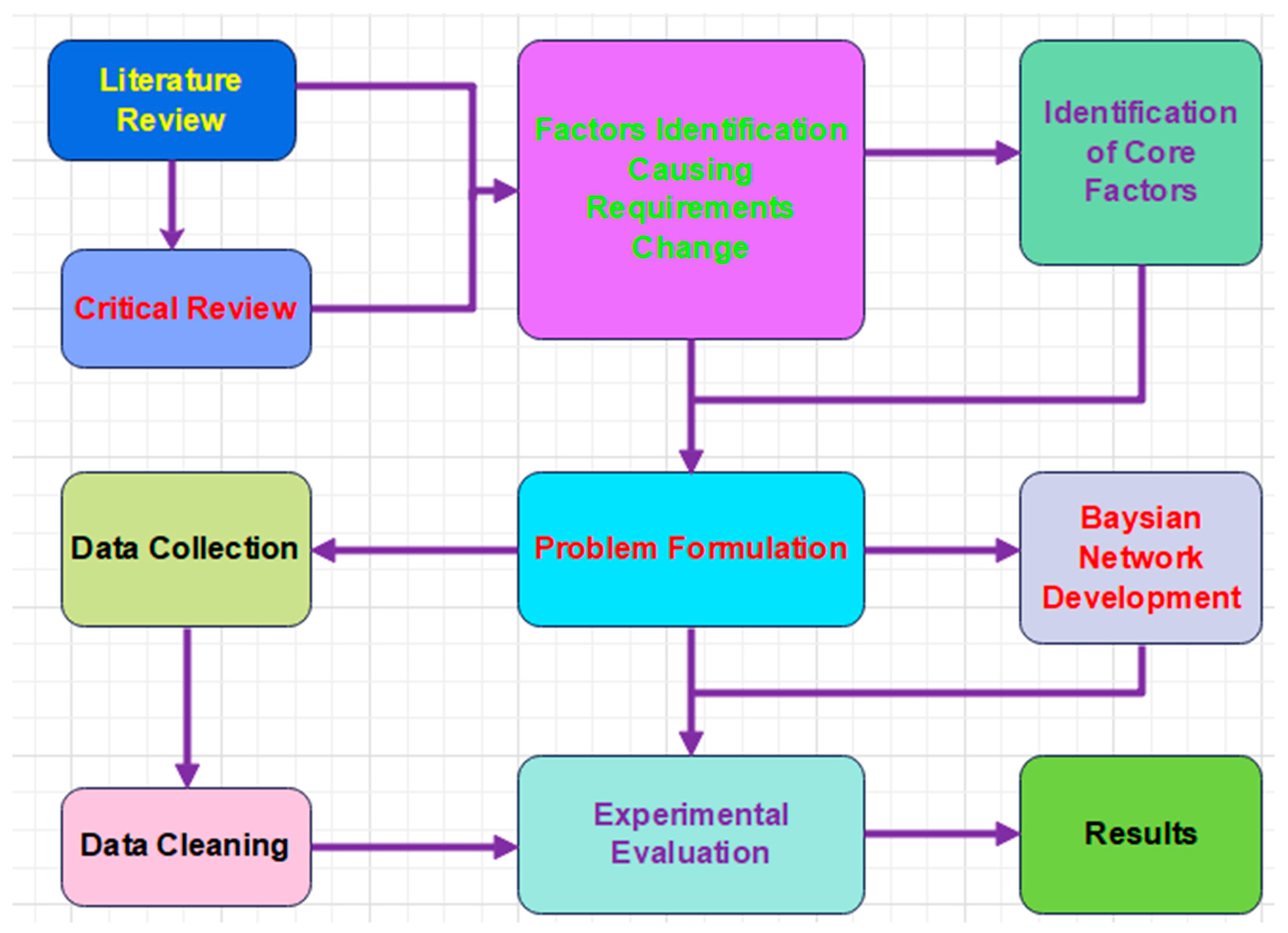
The methodology of the proposed approach is presented in Figure 1. After the detailed literature review, the core factors/variables that led to the research problem were introduced. According to the problem, the study presents a probabilistic Bayesian model for variable change predictions. We gathered data against these variables and integrated them into the model.
3.1. Data Collection
To evaluate the proposed system, a questionnaire was used for data collection. Certain software requirements were framed on the questionnaire and distributed online to experts for rating. Data were collected from the system analysts, stakeholders, quality assurance experts, and developers. As criteria, experts must have at least two years of experience in software engineering; likewise, developers should have at least one year of experience in software development, and system analysts should have one year of experience in requirement engineering.
The questionnaire’s first section describes the aims and objectives of data collection and the variables on which the requirement probability will be measured. In the second section, the directions about the questionnaire are given, and in the third section, requirements are given along with the questions related to each variable. The respondents have to respond on the scale along with each question. The scale was organized as follows: 1: very low, 2: low, 3: high, and 4: very high. The scale was used for rating the particular requirements, which shows the probability value estimated by respondents. The dataset comprises the responses of the system analysts, developers, and quality assurance experts on the requirements of the online registration system. The dataset ensures a minimum of three hundred responses.
After obtaining responses, the probability of each variable is calculated. We assign weights to each person’s response according to their knowledge and expertise. As the experts have a high experience and knowledge in the domain, we assigned a 50% weightage to their responses. Likewise, we assigned a 30% weight to the system analysts and a 20% weightage to the developers.
3.2. Data Analysis
The information was gathered in an Excel spreadsheet; whereas for data analysis, IBM SPSS Statistics Version 27.0.0.0 was used to clean and analyze the data. The data’s mean, median, mode, variance, standard deviation range, and missing values were examined using descriptive analysis.
Table 2 presents the results of descriptive analysis. It shows the mean, median, mode, variance, standard deviation, and missing values of the variables.
We applied a normalization test to determine whether the data were normally distributed. The findings are statistically significant since all alpha values (p-value) were less than 0.05 (there is a less than 5% chance that the data being tested have an error). Moreover, we also analyzed the relationship between the dependent and independent variables by determining their correlation and regression.
Table 3 demonstrates how close the proposed model is to the regression line, as the values are between 0 and 100%; thus, these are best fitted to the model. The table shows that the values are significant, as they are below the alpha value (0.05). As the regression values validate the fitness of the model and the relation between variables, we will utilize them in calculating the conditional probabilities between variables.
3.3. Bayesian Network Construction with Netica
Data collected from experts, stakeholders, and developers aided in developing the Bayesian network. In a Bayesian network, each node represents a separate variable (v1, v2, …, vn), and the graph itself is a directed acyclic graph. Relationships between these variables are represented by the arcs that connect them. The joint probability distribution is found by multiplying the individual conditional probabilities associated with each variable.
In a Bayesian network, the posterior probability of a particular variable is calculated using the inference process. The conditional probability of variables was obtained from experts, stakeholders, and developers by defining the probability scale and taking the averages.
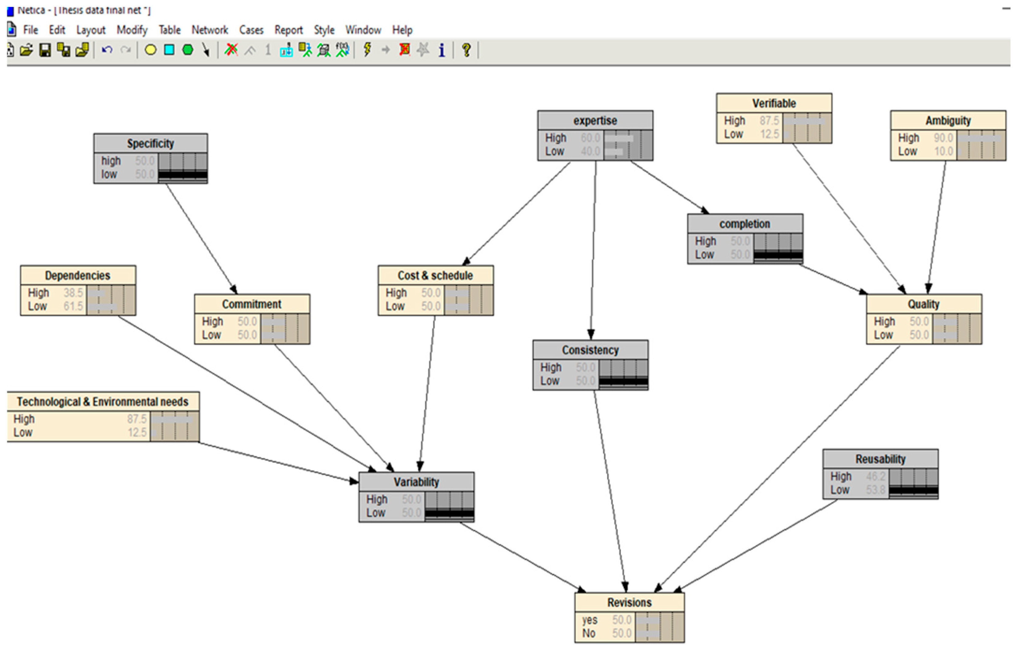
The proposed Bayesian network is constructed using the Netica tool. The Netica tool develops the considered Bayesian network by incorporating expert knowledge to obtain the conditional probabilities. By inputting the variables’ prior probabilities and running the tool, Netica determines the variables’ posterior probabilities. The model can learn the Excel data file to perform the inference in Netica. Figure 2 presents the construction of the Bayesian network over Netica.
In this network, the dependent variables are commitment, cost and schedule, quality, consistency, variability, and revisions. Furthermore, the independent variables are specificity, dependencies, technological needs, expertise, verifiable, ambiguity, completion, and reusability. The initial probability values of nodes are set to low, and high. By selecting the states, the dialog box is settled to discrete variables. The probability is measured in percentage for each variable. To perform the inference, the model is made capable of learning. For this purpose, an Excel data sheet is incorporated into Netica, which has the same name as the nodes and the frequency associated with the nodes. When the file is added into Netica, it will set the conditional probabilities in tables by reading the file. The data of the high and low states of the node variables are incorporated from the case file. Compiling and incorporating the different case files will provide the results for different states.
3.4. Proposed Prediction Model
Referencing the literature, algorithm-based research works are more effective in requirement change prediction. Thus, we measured the existing algorithm performance by incorporating our proposed dataset. Certain case studies have used a variable elimination algorithm to determine the variables’ posterior probabilities. For example, Zhang et al. [36] proposed this method to calculate the posterior marginal probabilities of the variables. As the Bayesian network comprises the factorization of joint probability into a product set of conditional probabilities, they convert the independence relation to or sum and or max by variable elimination. This algorithm provides the probability values of the queried variable.
Variable Elimination Algorithm
The variable elimination algorithm takes the joint probability of all of the variables and sums out all of the variables to obtain the marginal probability of a single queried variable. In this method, two procedures are used: describing the order of variables and eliminating a single variable from the group.
The first procedure is to describe the order of variables. At this stage, the variables present in the Bayesian network are listed in order of elimination.
The second procedure eliminates a single variable from the group of factors and returns a single factor. All algebraic operations are performed in the second phase to eliminate the variables. Algorithm 1 presents the pseudocode of the variable elimination.
| Algorithm 1 | Variable elimination algorithm | |||
| Input data: | ||||
| φ: Set of factors. | ||||
| F: Stack having an active list of factors. | ||||
| Z: Set of variables to be eliminated. | ||||
| K: Number of selected routes. | ||||
| Step 1. | Zi to Zk shows the order of variables. | |||
| For (i = 1; i ≤ k; i++) | ||||
| F←Sum-Product Eliminate Var (F, Zi); | ||||
| End for | ||||
| Step 2. | Subroutine sum over the product of all variable factors to eliminate and return the new factor. | |||
| φ * ← ∏ φ ∈ F (φ) | ||||
| Return φ * | ||||
| Procedure Sum-product eliminate Var () | ||||
| F′ = define all terms having argument Zi (variable to be eliminated) | ||||
| F′ ← {φ ∈ F: Z ∈ scope[φ]} | ||||
| F″ = remaining stack elements | ||||
| F″ = F-F’ | ||||
| Step 3. | Take the product of all factors in F′. | |||
| ψ ← ∏φ ∈ F′ φ | ||||
| Step 4. | Take the sum of products by eliminating Z. | |||
| T = new factor | ||||
| T ← ∑Z ψ | ||||
| Step 5. | Join the T with the remaining stack F″. | |||
| return F″ ∪ {T} | ||||
| Step 6. | End. | |||
The algorithm takes conditional probabilities as an input and then performs the factorization process. The second step includes the multiplication and marginalization of the factors, and in the next phase, the sum-out operation is performed to eliminate the variables from the set of factors. In the sum-out operation, the algorithm first marginalizes the variables by multiplying all factors, then draws a variable from a factor group and returns the factor with the remaining variables. We have incorporated the Bayesian network variables into the variable elimination algorithm to determine the posterior probability of revisions in the Bayesian network. We have taken the online registration system’s requirements and the defined variables reflecting the requirements’ nature. The Bayesian network is integrated into the algorithm by adding the conditional probabilities of each variable node with its parent. The algorithm takes the values and performs all of the necessary operations.
3.5. Proposed Prediction Algorithm
The proposed algorithm for predicting queried variables is introduced in Algorithm 2. The proposed prediction model utilizes the variable elimination method.
All elements’ probabilities are obtained by merging and taking averages of the stakeholders’, experts’, and developers’ data values. The first while loop takes all elements in the algorithm and calculates the conditional probability values. It checks whether the variable belongs to a stakeholder, developer, or expert, and it checks the regression R square value between the data. If the values are between 1 and 100, then it calculates the final value of conditional probability by multiplying it with the regression values and the weights assigned to each person. We assigned a 30% weightage to stakeholders’ data, 20% to developers’ data, and 50% to experts’ data. The second loop takes the conditional probability values of all of the variables and builds factors, and the variable elimination code returns the final probability value for the goal variable.
| Algorithm 2 | Proposed prediction algorithm | ||
| Step 1. | Def Proposed Algorithm (cond_Prob) | ||
| { | |||
| Vi = initial variable | |||
| Vn = Total number of variables | |||
| While (Vi ≤ Vn) | |||
| { | |||
| Step 2. | If (Vi € Stakeholder. Dataset & Vi. RSquare Value > 1 & ≤100) | ||
| Cond_Prob1 = VI. Data*0.3*RSquare Value | |||
| Else | |||
| if (Vi € Developer. Dataset & Vi. RSquare Value >1 & ≤100) | |||
| Cond_Prob2= Vi. Data*0.2*RSquare Value | |||
| Else (Vi € Expert. Dataset & Vi. RSquare Value >1 & ≤100) | |||
| Cond_Prob3= Vi. Data*0.5*RSquare Value | |||
| FinalCond_Prob = merge (Cond_Prob1, Cond_Prob2, Cond_Prob3) | |||
| Step 3. | While (FinalCond_Probi ≤ FinalCond_Prob n) | ||
| { | |||
| F = Make Factors (FinalCond_Probi) | |||
| { | |||
| Step 4. | Variable Elimination (F, Vi); | ||
| Step 5. | Return cond_Prob; | ||
| Step 6. | End. | ||
3.6. Process Model
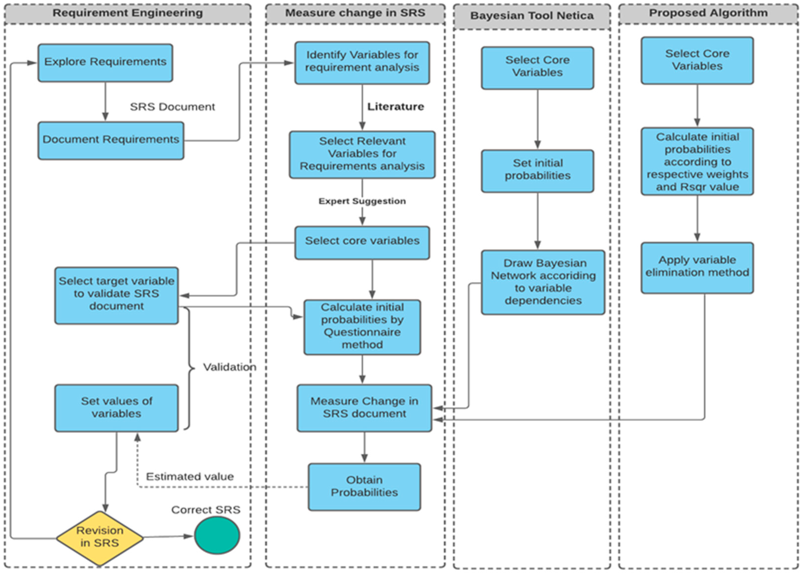
The requirements for the student’s management software were gathered and documented. The Software Requirement Specification (SRS) document should be complete and defined so that the actual requirements of the software can be fulfilled. The biggest issue in software development is a change in the SRS document and, to tackle this problem, we performed certain processes on each module. A complete process model of the proposed approach is presented in Figure 3.
Requirements are repeatedly passed from the complete cycle to measure the change in the requirement specification document. First, the requirements were gathered and explored for students’ management software. The requirements were listed in a document called the SRS document. After that, we identified the variables for analyzing the requirements. We analyzed the variables that support change predictions in the requirements document from the literature. We derived the core productive variables from experts’ suggestions and requirements engineers from relevant variables. The selected core variables measure the probability of change as follows.
- Measuring the posterior probability of target variables, e.g., revisions upon the effect of all of the core variables in the network.
- Measuring the posterior probability of the target variable in different scenarios, e.g., by making the individual variable evidence value high or low.
The initial probability was calculated by collecting data with the questionnaire method, as discussed above. In this regard, a Bayesian tool (Netica) was utilized, in which the network is constructed according to the variables’ dependencies, and measured the target variable’s posterior probability. The posterior probability was also measured by an algorithmic method utilizing the variable elimination method. The initial probability was calculated by multiplying the probabilities by the regression value of the variables and by the opinion weights of the developers, stakeholders, and experts discussed in the data collection section. After measuring the posterior probability, if there is a high probability of change, the revision in the requirements document will be high, and it is again fed back to the requirement-gathering phase.
4. Evaluation Measures
For the evaluation of the proposed methodology, we have used different evaluation measures. Detail is given in the following subsections.
4.1. Performance Evaluation
To measure the performance of the proposed work, algorithms were implemented in the Python language. Where all major functions were performed in the Net and Factor classes inherited in the main class. To compute the joint probability of all variables, a Bayesian network was constructed. Conditional probability values were given as a dataset in the form of a Jason file and on the run time. High and low evidence values were queried to compute the results of the desired variables along with the computation of the posterior probability.
4.1.1. Bayesian Network of Proposed Work
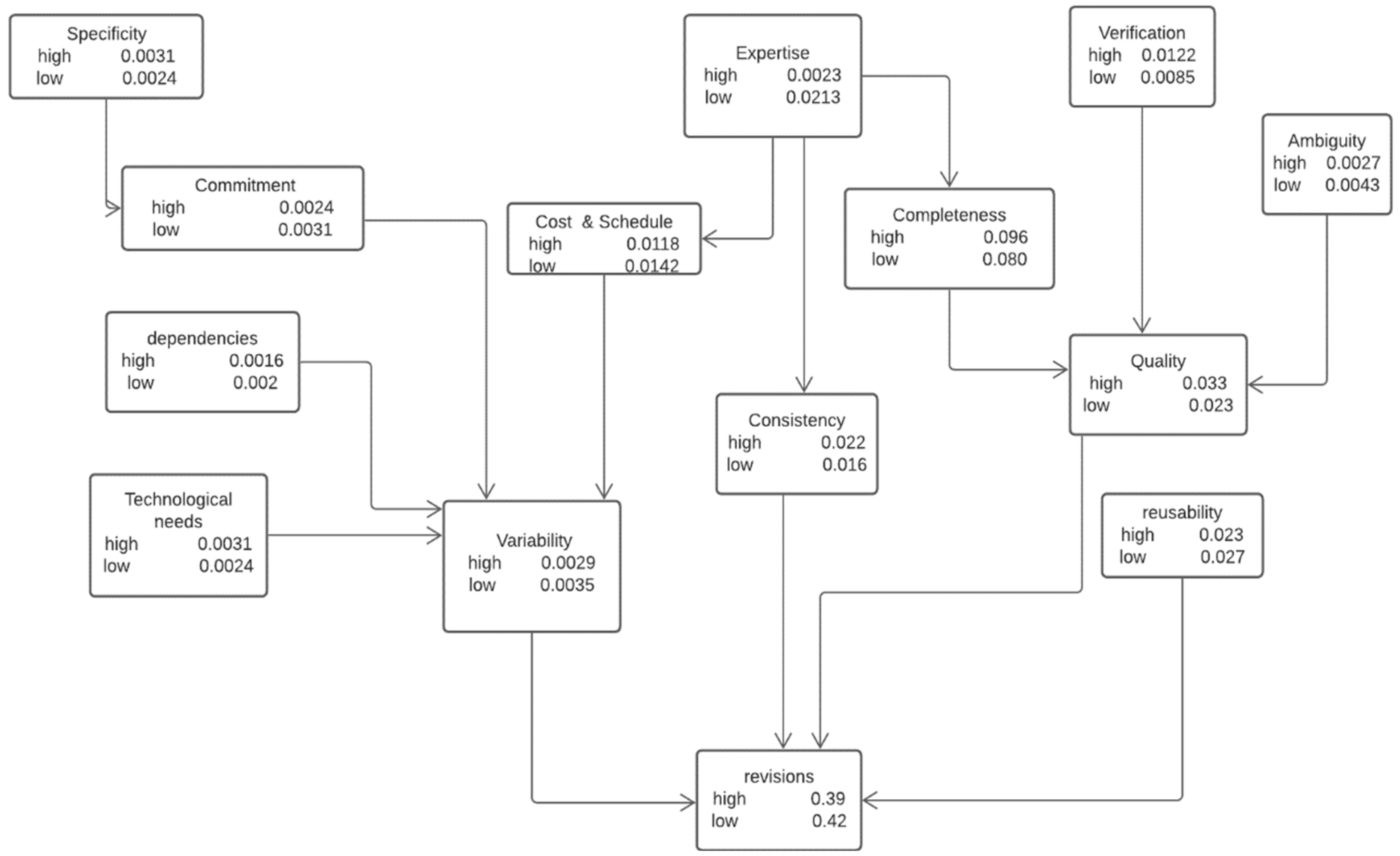
The variables represent the network’s degree of revisions; therefore, the posterior probability of each variable was computed in different cases and each time, and the results were recorded. The final form of the Bayesian network is presented in Figure 4. In this network, the proposed algorithm calculates the conditional probabilities of all of the variables and the posterior probability of revisions.
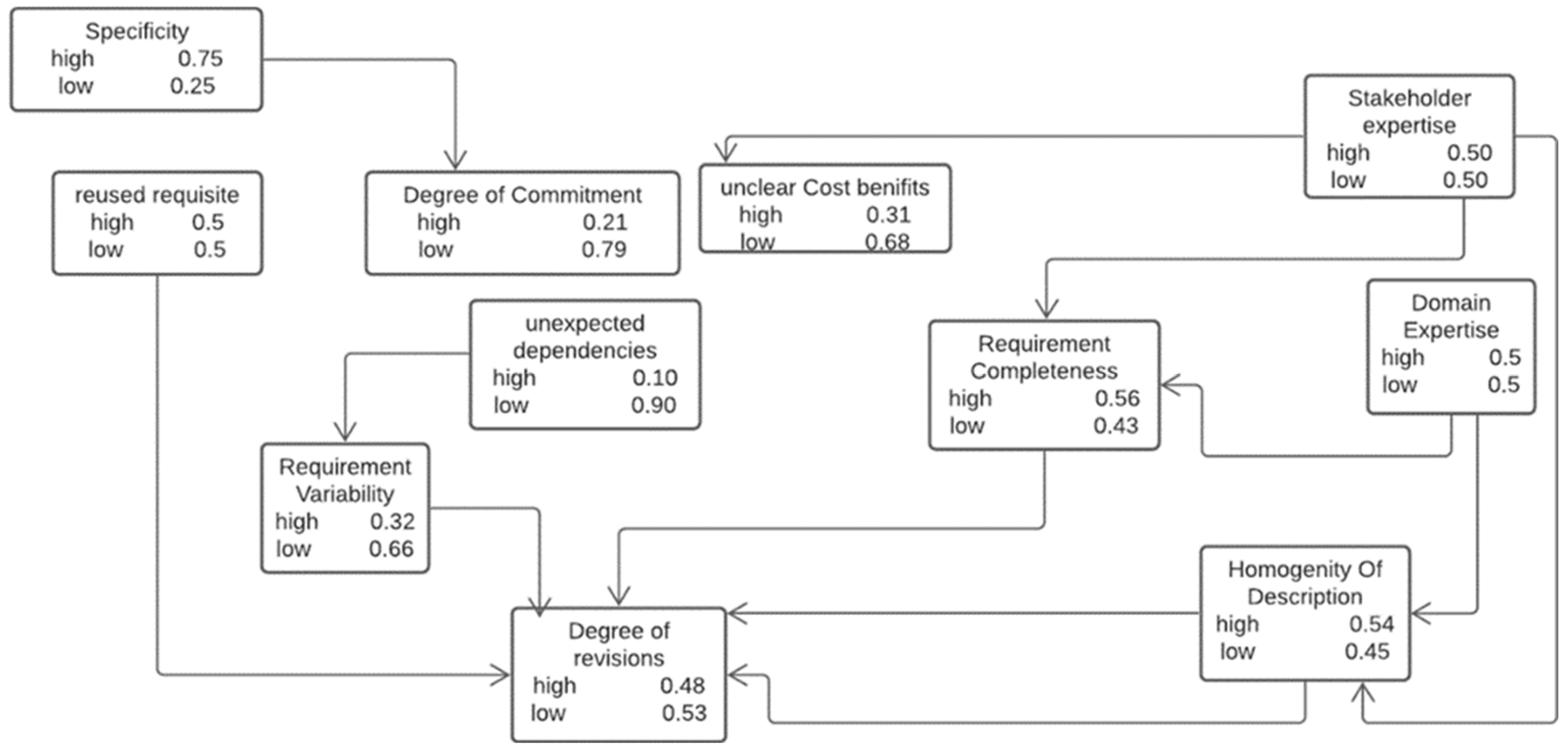
4.1.2. Bayesian Network of del Sagrado et al. [13]
To compare the results of the proposed model with a state-of-the-art method, the network model of del Sagrado et al. [13] was also constructed. In this regard, we compared the results of both models by incorporating the same dataset values. The del Sagrado et al. [13] model is described in Figure 5.
The results demonstrate a clear difference in the results of both networks. The del Sagrado et al. [13] network produced a 0.48 probability for the “high” state and a 0.53 probability for the “low” state regarding the data gathered from experts. Likewise, the results of the proposed network were a 0.39 probability for the “high” state and a 0.42 probability for the “low” state using the same dataset.
4.1.3. Sensitivity Analysis
We calculated the posterior probability of the target variable by increasing the values of the prior probabilities of the variables in the network. We increased the conditional probabilities of the variables dependent on the target node and analyzed the value of the target variable. The formula for the sensitivity analysis is given as:
where D (Pr, Pr’) is the distance between the old and new conditional probability values. While is a ratio of the old and new conditional probabilities of the low state probability, is the ratio of the old and new conditional probabilities of the high state probability.
D (Pr, Pr’) = ln min (Pr’x/v)/(Pr x/v) − ln max (Pr’x/v)/(Pr x/v)
P𝑒^(−𝑑)/P𝑒^(−𝑑) − P +1 <= Pr’(ą/ß) <= P𝑒^(𝑑)/P𝑒^(𝑑) − P + 1
Equation (2) shows the range of new probabilities of revisions where Pr’(ą/ß) is a new probability of revisions after changing the conditional probability values of the variable in the network. P𝑒^(−𝑑)/P𝑒^(−𝑑) − P + 1 is the low probability state of revisions and d is the distance calculated by Equation (1). Similarly, P𝑒^(−𝑑)/P𝑒^(−𝑑) − P + 1 is the low probability state of revisions, and d is the distance calculated by Equation (1).
The probabilities (before and after the increase) of variables (quality, reusability, variability, and consistency) are presented in Table 4. The distance between the old probability values of the variables is calculated by Equation (1) and the new probability of revision is calculated by Equation (2).
The revisions in the Bayesian network are dependent on the quality, reusability, variability, and consistency. To analyze the effect of the revisions, the conditional probabilities were increased by 5% (suggested by experts). Table 4 shows the results of the posterior probability of revisions as a result of increasing the probability of the given variables. The results demonstrate that there is little effect on the posterior probability, except in the variability values of 0.38 for the low state and 0.62 for the high state.
4.2. Accuracy Measurement
In this section, the accuracy values of the del Sagrado et al. [13] model and the proposed model are computed by the mean magnitude error (Equation (3)) and root mean square error (Equation (4)).
where n is the sample size, yi represents the actual results, and yi’ represents the estimated results.
MRE = 1/n │∑Actual Revisions − Estimated Revision/Actual Revisions│= 1/n │∑ yi − yi’/yi│
MSE = 1/n √(Actual Revisions − Estimated Revision)^2
The computed values are presented in Table 5 for comparison.
Low values of the root mean square error and mean magnitude relative error mean a higher accuracy of predictions. The lower the number of revisions, the higher the reliability of the requirement specification document. The values of the MMRE and RMSE of the proposed model are 0.0042 and 0.0026, while the MMRE and RMSE values of del Sagrado et al. [13] are 0.0052 and 0.0032. As the proposed model MMRE and RMSE values are lower than the del Sagrado et al. [13] model, the proposed model achieved a higher performance than the existing model.
4.3. Experimental Results and Discussion
In this section, the results of the experiment are listed in Table 6. These results are obtained by the variable elimination algorithm which takes the Bayesian network conditional probability values as its input. The Bayesian network is constructed to predict the revisions in the requirement specification document. Thus, the output results show the probability value of revisions. It has two values: “high” and “low”. Thus, it calculates the total probability on the basis of the conditional probabilities of the variables in the network. We also have shown the effects of the queried variables’ results on the individual variable values. Table 6 provides the results of the proposed approach.
We also analyzed the effects on the revision probability by varying the values of individual variables. We also applied this method to the del Sagrado et al. [13] prediction model and analyzed the results by comparing them with our proposed model results. We derived the results from the proposed model by making each variable probability high and low. The main purpose was to analyze the effect on the probability of revisions by varying each variable probability value. The results of the del Sagrado et al. [13] model on their proposed variables and acquired data are presented in Table 7.
The results obtained from both models by varying the values of each variable depict that the probability of revisions remains low in the proposed model as compared to the del Sagrado et al. [13] model. We also proposed two scenarios with experts’ suggestions for the prediction of revisions in the SRS document and recorded the results. The scenarios are as follows:
- Scenario 1: Specificity = High, Expertise = High, Verification = High, Ambiguity = Low, Dependency = Low, Technology = High, Completeness = High, Reusability = High, Commitment = High, Cost and Schedule = Low, Consistency = High, Quality = High, Variability = Low, Revisions = Low.
- Scenario 2: Specificity = Low, Expertise = Low, verification = Low, Ambiguity = High, Dependency = High, Technology = Low, completeness = Low, Reusability = Low, Commitment = Low, Cost and Schedule = High, Consistency = High, Quality = High, Variability = High, Revisions = High.
The results of the proposed model and the del Sagrado et al. [13] model after applying both scenarios are presented in Table 8.
After comparing the results of both tables, we concluded that when the variability value is high, our proposed model calculated a 0.42 and 0.45 probability of revisions for both scenarios. Likewise, in the del Sagrado et al. [13] model results table, when the requirement variability is high, it calculated a 0.51 probability of revisions; when it is low, it calculated a 0.44 probability of revisions. From the results, it is observed that there is a minor difference in the values of both models. However, the proposed model’s results are lower in each scenario, which means that the proposed model is better than that of del Sagrado et al. [13].
In this section, the proposed model is evaluated by (i) comparing results, (ii) sensitivity analysis, and (iii) accuracy calculation. We performed a sensitivity analysis by using four variables to measure the effects on the posterior probability of revisions. The accuracy of the proposed model is calculated through two methods: (i) mean magnitude relative error and (ii) root mean square error. The MMRE and RMSE values of the proposed model are 0.0042 and 0.0026, while the MMRE and RMSE values of del Sagrado et al. [13] are 0.0052 and 0.0032, respectively. As lower values are better, it is concluded that the proposed model has a better accuracy.
5. Conclusions and Future Work
Requirement change is a big challenge in the software industry. The change in requirements document at the design and implementation level is a major cause of increases in the project cost and time, and low quality which leads to software failures. Thus, this issue should be resolved in the early stages. In this work, we have focused on predicting the change in the requirement specification document. We performed a detailed systematic literature review to find the variables that can be used for the accurate prediction of changes in requirements. We observed that existing approaches use a few variables for change predictions resulting in compromised accuracy, whereas relatively few approaches consider expert knowledge and requirements matrices. Thus, in this work, we discovered the core factors from the literature that are the most influential on the revision of requirement specifications and utilized them in the construction of the Bayesian network. We incorporated artificial intelligent techniques into software engineering for making decisions based upon stakeholders’, developers’, and experts’ knowledge in the Bayesian network. We collected data by the questionnaire method to take the responses of all of the persons concerned. Their responses were compiled in an Excel file. After that, the dataset was used to perform a detailed quantitative analysis. We constructed a Bayesian network with the help of the Netica tool and examined the posterior probability of revisions by a variable elimination algorithm. Later on, the Bayesian network was incorporated into the variable elimination algorithm. The Bayesian network contains the conditional probabilities of the independent and dependent variables. We evaluated the Bayesian network by the comparison method, sensitivity analysis, and accuracy calculation. The results show that the del Sagrado et al. [13] model obtained a 0.44 probability for low-state revisions and a 0.51 probability value for high-state revisions, whereas the proposed model’s low-state revisions probability is decreased to 0.42, and the high-state revisions probability decreased to 0.45. This means, that the proposed method has computed significant results. Hence, we can conclude that if the proposed method is applied to the requirement specification document, the requirement change can be predicted, which may direct the project manager to take corrective or preventive measures. In the future, we want to repeat the same experiment using a consistent dataset. Presently, we utilized one algorithm for obtaining the posterior probability. In the future, we will use other methods and algorithms for computing the change probability and analyzing the performance. Finally, we also want to test the proposed model in a real scenario.
Author Contributions
Conceptualization, R.F., F.Z., M.H., I.F., A.A.A. and H.A.A.; data curation, R.F., F.Z., A.A., M.H., I.F., A.A.A. and H.A.A.; formal analysis, R.F., F.Z., A.A., I.F., A.A.A. and H.A.A.; funding acquisition, I.F., A.A.A. and H.A.A.; investigation, R.F., F.Z., A.A., M.H., I.F., A.A.A. and H.A.A.; methodology, R.F., F.Z., A.A., M.H., I.F., A.A.A. and H.A.A.; project administration, R.F., F.Z., A.A., M.H., A.A.A. and H.A.A.; resources, R.F., F.Z., A.A., M.H., I.F., A.A.A. and H.A.A.; software, R.F., F.Z., A.A., M.H., I.F., A.A.A. and H.A.A.; supervision, R.F., F.Z., A.A., M.H., I.F., A.A.A. and H.A.A.; validation R.F., F.Z., A.A., M.H., I.F., A.A.A. and H.A.A.; visualization, R.F., F.Z., A.A., M.H., I.F., A.A.A. and H.A.A.; writing—original draft, R.F., F.Z., A.A., M.H., I.F., A.A.A. and H.A.A.; writing—review and editing, R.F., F.Z., A.A., M.H., I.F., A.A.A. and H.A.A. All authors have read and agreed to the published version of the manuscript.
Funding
This work was supported by the Princess Nourah bint Abdulrahman University Researchers Supporting Project, number (PNURSP2023R 308), Princess Nourah bint Abdulrahman University, Riyadh, Saudi Arabia.
Data Availability Statement
Not applicable.
Acknowledgments
The authors extend their appreciation to the Princess Nourah bint Abdulrahman University Researchers Supporting Project, number (PNURSP2023R 308), Princess Nourah bint Abdulrahman University, Riyadh, Saudi Arabia.
Conflicts of Interest
The authors declare no conflict of interest.
References
- Ciancarini, P.; Farina, M.; Okonicha, O.; Smirnova, M.; Succi, G. Software as Storytelling: A Systematic Literature Review. Comput. Sci. Rev. 2023, 47, 100517. [Google Scholar] [CrossRef]
- Shwetha, A.N.; Sumathi, R.; Prabodh, C.P. A Survey on Mobile Application Development Models. In Mobile Application Development: Practice and Experience; Springer Nature Singapore: Singapore, 2023; pp. 1–9. ISBN 9789811968921. [Google Scholar]
- Lin, B.; Cassee, N.; Serebrenik, A.; Bavota, G.; Novielli, N.; Lanza, M. Opinion Mining for Software Development: A Systematic Literature Review. ACM Trans. Softw. Eng. Methodol. 2022, 31, 1–41. [Google Scholar] [CrossRef]
- Mihelič, A.; Vrhovec, S.; Hovelja, T. Agile Development of Secure Software for Small and Medium-Sized Enterprises. Sustainability 2023, 15, 801. [Google Scholar] [CrossRef]
- Thota, M.K.; Shajin, F.H.; Rajesh, P. Survey on Software Defect Prediction Techniques. Int. J. Appl. Sci. Eng. 2020, 17, 331–344. [Google Scholar]
- Yang, Y.; Xia, X.; Lo, D.; Bi, T.; Grundy, J.; Yang, X. Predictive Models in Software Engineering: Challenges and Opportunities. ACM Trans. Softw. Eng. Methodol. 2022, 31, 1–72. [Google Scholar] [CrossRef]
- Baham, C.; Hirschheim, R. Issues, Challenges, and a Proposed Theoretical Core of Agile Software Development Research. Inf. Syst. J. 2022, 32, 103–129. [Google Scholar] [CrossRef]
- Karagiannis, D. Conceptual Modelling Methods: The AMME Agile Engineering Approach. In Domain-Specific Conceptual Modeling; Springer International Publishing: Cham, Switzerland, 2018; pp. 3–21. ISBN 9783030935467. [Google Scholar]
- Yang, Y.; Xia, X.; Lo, D.; Grundy, J. A Survey on Deep Learning for Software Engineering. ACM Comput. Surv. 2022, 54, 1–73. [Google Scholar] [CrossRef]
- Khaliq, Z.; Farooq, S.U.; Khan, D.A. Artificial Intelligence in Software Testing: Impact, Problems, Challenges and Prospect. arXiv 2022, arXiv:2201.05371. [Google Scholar]
- Huang, Y.-S.; Chiu, K.-C.; Chen, W.-M. A Software Reliability Growth Model for Imperfect Debugging. J. Syst. Softw. 2022, 188, 111267. [Google Scholar] [CrossRef]
- Zhao, Z.; Zhang, L.; Lian, X.; Gao, X.; Lv, H.; Shi, L. ReqGen: Keywords-Driven Software Requirements Generation. Mathematics 2023, 11, 332. [Google Scholar] [CrossRef]
- del Sagrado, J.; del Águila, I.M. Stability Prediction of the Software Requirements Specification. Softw. Qual. J. 2018, 26, 585–605. [Google Scholar] [CrossRef]
- Park, S.; Maurer, F.; Eberlein, A.; Fung, T.-S. Requirements Attributes to Predict Requirements Related Defects. In Proceedings of the 2010 Conference of the Center for Advanced Studies on Collaborative Research—CASCON ’10, Toronto, ON, Canada, 1–4 November 2010; ACM Press: New York, NY, USA, 2010. [Google Scholar]
- Hein, P.H.; Voris, N.; Morkos, B. Predicting Requirement Change Propagation through Investigation of Physical and Functional Domains. Res. Eng. Des. 2018, 29, 309–328. [Google Scholar] [CrossRef]
- Arora, C.; Sabetzadeh, M.; Goknil, A.; Briand, L.C.; Zimmer, F. Change Impact Analysis for Natural Language Requirements: An NLP Approach. In Proceedings of the 2015 IEEE 23rd International Requirements Engineering Conference (RE), Ottawa, ON, Canada, 24–28 August 2015; IEEE: New York, NY, USA, 2015; pp. 6–15. [Google Scholar]
- Yadav, H.B.; Yadav, D.K. Early Software Reliability Analysis Using Reliability Relevant Software Metrics. Int. J. Syst. Assur. Eng. Manag. 2017, 8, 2097–2108. [Google Scholar] [CrossRef]
- Bano, M. Addressing the Challenges of Requirements Ambiguity: A Review of Empirical Literature. In Proceedings of the 2015 IEEE Fifth International Workshop on Empirical Requirements Engineering (EmpiRE), Ottawa, ON, Canada, 24 August 2015; IEEE: New York, NY, USA, 2015; pp. 21–24. [Google Scholar]
- Zheng, W.; Shen, T.; Chen, X.; Deng, P. Interpretability Application of the Just-in-Time Software Defect Prediction Model. J. Syst. Softw. 2022, 188, 111245. [Google Scholar] [CrossRef]
- Wakimoto, M.; Morisaki, S. Goal-Oriented Software Design Reviews. IEEE Access 2022, 10, 32584–32594. [Google Scholar] [CrossRef]
- Butt, S.A.; Khalid, A.; Ercan, T.; Ariza-Colpas, P.P.; Melisa, A.-C.; Piñeres-Espitia, G.; De-La-Hoz-Franco, E.; Melo, M.A.P.; Ortega, R.M. A Software-Based Cost Estimation Technique in Scrum Using a Developer’s Expertise. Adv. Eng. Softw. 2022, 171, 103159. [Google Scholar] [CrossRef]
- Rath, A.K. Fundamentals of Software Engineering: Designed to Provide an Insight into the Software Engineering Concepts (English Edition); BPB Publications: New Delhi, India, 2020; ISBN 9789388511773. [Google Scholar]
- Devanbu, P.; Dwyer, M.; Elbaum, S.; Lowry, M.; Moran, K.; Poshyvanyk, D.; Ray, B.; Singh, R.; Zhang, X. Deep Learning & Software Engineering: State of Research and Future Directions. arXiv 2020, arXiv:2009.08525. [Google Scholar]
- Bibiano, A.C.; Uchôa, A.; Assunção, W.K.G.; Tenório, D.; Colanzi, T.E.; Vergilio, S.R.; Garcia, A. Composite Refactoring: Representations, Characteristics and Effects on Software Projects. Inf. Softw. Technol. 2023, 156, 107134. [Google Scholar] [CrossRef]
- Zorzetti, M.; Signoretti, I.; Salerno, L.; Marczak, S.; Bastos, R. Improving Agile Software Development Using User-Centered Design and Lean Startup. Inf. Softw. Technol. 2022, 141, 106718. [Google Scholar] [CrossRef]
- Laplante, P.A.; Kassab, M. Requirements Engineering for Software and Systems, 4th ed.; Auerbach: London, UK, 2022; ISBN 9781000593792. [Google Scholar]
- Hou, F.; Jansen, S. A Systematic Literature Review on Trust in the Software Ecosystem. Empir. Softw. Eng. 2023, 28, 8. [Google Scholar] [CrossRef]
- Kadebu, P.; Sikka, S.; Tyagi, R.K.; Chiurunge, P. A Classification Approach for Software Requirements towards Maintainable Security. Sci. Afr. 2023, 19, e01496. [Google Scholar] [CrossRef]
- Sur, T.; Jaisswal, A.; Vinayakarao, V. Mathematical Expressions in Software Engineering Artifacts. In Proceedings of the Proceedings of the 6th Joint International Conference on Data Science & Management of Data (10th ACM IKDD CODS and 28th COMAD), Mumbai, India, 4–7 January 2023; ACM: New York, NY, USA, 2023. [Google Scholar]
- Laato, S.; Mäntymäki, M.; Islam, A.K.M.N.; Hyrynsalmi, S.; Birkstedt, T. Trends and Trajectories in the Software Industry: Implications for the Future of Work. Inf. Syst. Front. 2022, 25, 929–944. [Google Scholar] [CrossRef]
- Horcas, J.M.; Pinto, M.; Fuentes, L. Empirical Analysis of the Tool Support for Software Product Lines. Softw. Syst. Model. 2023, 22, 377–414. [Google Scholar] [CrossRef]
- Weder, B.; Barzen, J.; Leymann, F.; Vietz, D. Quantum Software Development Lifecycle. In Quantum Software Engineering; Springer International Publishing: Cham, Switzerland, 2022; pp. 61–83. ISBN 9783031053238. [Google Scholar]
- Akbar, M.A.; Smolander, K.; Mahmood, S.; Alsanad, A. Toward Successful DevSecOps in Software Development Organizations: A Decision-Making Framework. Inf. Softw. Technol. 2022, 147, 106894. [Google Scholar] [CrossRef]
- Nandakumar, R. Quantitative Quality Score for Software. In Proceedings of the 15th Innovations in Software Engineering Conference, Gandhinagar, India, 24–26 February 2022; ACM: New York, NY, USA, 2022. [Google Scholar]
- Gutfleisch, M.; Klemmer, J.H.; Busch, N.; Acar, Y.; Sasse, M.A.; Fahl, S. How Does Usable Security (Not) End up in Software Products? Results from a Qualitative Interview Study. In Proceedings of the 2022 IEEE Symposium on Security and Privacy (SP), San Francisco, CA, USA, 23–25 May 2022; IEEE: New York, NY, USA, 2022; pp. 893–910. [Google Scholar]
- Xiang, Y.; Loker, D. Trans-Causalizing NAT-Modeled Bayesian Networks. IEEE Trans. Cybern. 2022, 52, 3553–3566. [Google Scholar] [CrossRef] [PubMed]
Figure 1.
Graphical representation of the proposed methodology.

Figure 2.
Bayesian network constructed in Netica.

Figure 3.
Process model of change prediction.

Figure 4.
Proposed Bayesian network.

Figure 5.
Bayesian network results of the del Sagrado et al. [13] model.
Figure 5.
Bayesian network results of the del Sagrado et al. [13] model.

Table 2.
Descriptive analysis of variables.
| Variables | Missing Values | Mean | Median | Mode | Standard Deviation | Variance | Range |
|---|---|---|---|---|---|---|---|
| Specificity | 1 | 2.7061 | 2.8 | 2.45 | 0.62 | 0.387 | 2.45 |
| Consistency | 2 | 2.7595 | 2.9 | 3.27 | 0.70 | 0.501 | 3.00 |
| Completion | 3 | 2.7965 | 2.8 | 2.00 | 0.66 | 0.448 | 2.45 |
| Ambiguity | 3 | 2.6476 | 2.60 | 2.00 | 0.71 | 0.509 | 2.82 |
| Commitment | 1 | 2.727 | 2.70 | 2.73 | 0.50 | 0.374 | 2.09 |
| Expertise | 3 | 2.7993 | 2.95 | 3.00 | 0.62 | 0.448 | 2.36 |
| Quality | 2 | 2.8282 | 2.90 | 2.09 | 0.61 | 0.359 | 2.19 |
| Reusability | 3 | 2.7730 | 2.79 | 3.36 | 0.66 | 0.380 | 2.36 |
| Dependency | 0 | 2.5329 | 2.58 | 2.00 | 0.59 | 0.343 | 2.55 |
| Variability | 2 | 2.5620 | 2.54 | 2.00 | 0.61 | 0.383 | 2.18 |
| Cost and schedule | 4 | 2.6354 | 2.8 | 2.00 | 0.66 | 0.340 | 2.82 |
| Verification | 2 | 2.7694 | 2.74 | 3.00 | 0.69 | 0.486 | 2.82 |
| Technological needs | 2 | 2.7830 | 2.75 | 3.09 | 0.66 | 0.445 | 2.55 |
Table 3.
Variables regression results.
| Independent Variables | Dependent Variables | R Square | Adjusted R Square | Co-Variance | Significant Value |
|---|---|---|---|---|---|
| Specificity | Commitment | 0.037 | 0.022 | 0.006 | 0.001 |
| Expertise | Consistency | 0.097 | 0.084 | 0.006 | 0.001 |
| Completeness | Quality | 0.067 | 0.054 | 0.010 | 0.001 |
| Ambiguity | Quality | 0.018 | 0.003 | 0.010 | 0.001 |
| Verification | Quality | 0.098 | 0.085 | 0.010 | 0.001 |
| Dependency | Variability | 0.010 | 0.014 | 0.016 | 0.001 |
| Technology | Variability | 0.016 | 0.001 | 0.024 | 0.001 |
| Expertise | Cost and schedule | 0.075 | 0.061 | 0.012 | 0.004 |
| Expertise | Completeness | 0.462 | 0.454 | 0.009 | 0.013 |
Table 4.
Posterior probability of revisions with respect to the sensitivity analysis.
| Variables | Low State Old Conditional Probability of Revisions | Low State New Conditional Probability of Revisions | High State Old ConditionalProbability of Revisions | High State New Conditional Probability of Revisions |
|---|---|---|---|---|
| Quality | 0.42 | 0.41 | 0.45 | 0.45 |
| Reusability | 0.42 | 0.41 | 0.45 | 0.46 |
| Consistency | 0.42 | 0.41 | 0.45 | 0.45 |
| Variability | 0.42 | 0.38 | 0.45 | 0.62 |
Table 5.
Results comparison between the proposed model and the del Sagrado et al. [13] model.
Table 5.
Results comparison between the proposed model and the del Sagrado et al. [13] model.
| Models | Mean Values of Estimated Results | Mean Magnitude Relative Error (MMRE) | Root Mean Square Error (RMSE) |
|---|---|---|---|
| Proposed model | 0.465 | 0.0042 | 0.026 |
| del Sagrado et al. [13] model | 0.435 | 0.0052 | 0.032 |
Table 6.
Results of the proposed model of individual variable effects on revisions.
| Variables | Probability Value | Probability (Revisions) | Probability Value | Probability (Revisions) |
|---|---|---|---|---|
| Specificity | High | 0.44 | Low | 0.45 |
| Expertise | High | 0.44 | Low | 0.45 |
| Verifiable | High | 0.44 | Low | 0.45 |
| Ambiguity | High | 0.45 | Low | 0.44 |
| Dependency | High | 0.45 | Low | 0.44 |
| Technology | High | 0.44 | Low | 0.45 |
| Completeness | High | 0.44 | Low | 0.45 |
| Reusability | High | 0.44 | Low | 0.45 |
| Commitment | High | 0.45 | Low | 0.44 |
| Cost and schedule | High | 0.45 | Low | 0.44 |
| Consistency | High | 0.44 | Low | 0.45 |
| Quality | High | 0.43 | Low | 0.44 |
| Variability | High | 0.42 | Low | 0.45 |
Table 7.
Results of the del Sagrado et al. [13] model individual variable effects on revisions.
Table 7.
Results of the del Sagrado et al. [13] model individual variable effects on revisions.
| Variables | Probability Value | Probability (Revision) | Probability Value | Probability (Revisions) |
|---|---|---|---|---|
| Specificity | High | 0.49 | Low | 0.52 |
| Stakeholder expertise | High | 0.49 | Low | 0.52 |
| Unexpected dependencies | High | 0.52 | Low | 0.49 |
| Requirement completeness | High | 0.49 | Low | 0.52 |
| Reused requisite | High | 0.49 | Low | 0.52 |
| Degree of commitment | High | 0.52 | Low | 0.49 |
| Unclear cost and benefits | High | 0.52 | Low | 0.49 |
| Homogeneity | High | 0.49 | Low | 0.52 |
| Requirement variability | High | 0.43 | Low | 0.49 |
Table 8.
Scenario results of the proposed model and the del Sagrado et al. [13] model.
Disclaimer/Publisher’s Note: The statements, opinions and data contained in all publications are solely those of the individual author(s) and contributor(s) and not of MDPI and/or the editor(s). MDPI and/or the editor(s) disclaim responsibility for any injury to people or property resulting from any ideas, methods, instructions or products referred to in the content. |
© 2023 by the authors. Licensee MDPI, Basel, Switzerland. This article is an open access article distributed under the terms and conditions of the Creative Commons Attribution (CC BY) license (https://creativecommons.org/licenses/by/4.0/).
Share and Cite
MDPI and ACS Style
Fatima, R.; Zeshan, F.; Ahmad, A.; Hamid, M.; Filali, I.; Alhussan, A.A.; Abdallah, H.A. Requirement Change Prediction Model for Small Software Systems. Computers 2023, 12, 164. https://doi.org/10.3390/computers12080164
AMA Style
Fatima R, Zeshan F, Ahmad A, Hamid M, Filali I, Alhussan AA, Abdallah HA. Requirement Change Prediction Model for Small Software Systems. Computers. 2023; 12(8):164. https://doi.org/10.3390/computers12080164
Chicago/Turabian StyleFatima, Rida, Furkh Zeshan, Adnan Ahmad, Muhamamd Hamid, Imen Filali, Amel Ali Alhussan, and Hanaa A. Abdallah. 2023. "Requirement Change Prediction Model for Small Software Systems" Computers 12, no. 8: 164. https://doi.org/10.3390/computers12080164
Note that from the first issue of 2016, this journal uses article numbers instead of page numbers. See further details here.