

Bound the Parameters of Neural Networks Using Particle Swarm Optimization


1
Department of Informatics and Telecommunications, University of Ioannina, 45110 Ioannina, Greece
2
Department of Engineering Informatics and Telecommunications, University of Western Macedonia, 50100 Kozani, Greece
*
Author to whom correspondence should be addressed.
Computers 2023, 12(4), 82; https://doi.org/10.3390/computers12040082
Submission received: 24 March 2023
/
Revised: 10 April 2023
/
Accepted: 15 April 2023
/
Published: 17 April 2023
(This article belongs to the Special Issue Uncertainty-Aware Artificial Intelligence)
Abstract
:Artificial neural networks are machine learning models widely used in many sciences as well as in practical applications. The basic element of these models is a vector of parameters; the values of these parameters should be estimated using some computational method, and this process is called training. For effective training of the network, computational methods from the field of global minimization are often used. However, for global minimization techniques to be effective, the bounds of the objective function should also be clearly defined. In this paper, a two-stage global optimization technique is presented for efficient training of artificial neural networks. In the first stage, the bounds for the neural network parameters are estimated using Particle Swarm Optimization and, in the following phase, the parameters of the network are optimized within the bounds of the first phase using global optimization techniques. The suggested method was used on a series of well-known problems in the literature and the experimental results were more than encouraging.
1. Introduction
Artificial neural networks (ANNs) are parametric machine learning models [1,2] which have been widely used during the last decades in a series of practical problems from scientific fields such as physics problems [3,4,5], chemistry problems [6,7,8], problems related to medicine [9,10], economic problems [11,12,13], etc. In addition, ANNs have recently been applied to models solving differential equations [14,15], agricultural problems [16,17], facial expression recognition [18], wind speed prediction [19], the gas consumption problem [20], intrusion detection [21], etc. Usually, neural networks are defined as a function , provided that the vector is the input pattern to the network and the vector stands for the weight vector. To estimate the weight vector, the so-called training error is minimized, which is defined as the sum:
In Equation (1), the values t define the training set for the neural network. The values denote the expected output for the pattern .
To minimize the quantity in Equation (1), several techniques have been proposed in the relevant literature such as the Back Propagation method [22,23], the RPROP method [24,25,26], Quasi Newton methods [27,28], Simulated Annealing [29,30], genetic algorithms [31,32], Particle Swarm Optimization [33,34], Differential Optimization methods [35], Evolutionary Computation [36], the Whale optimization algorithm [37], the Butterfly optimization algorithm [38], etc. In addition, many researchers have focused their attention on techniques for initializing the parameters of artificial neural networks, such as the usage of decision trees to initialize neural networks [39], a method based on Cachy’s inequality [40], usage of genetic algorithms [41], initialization based on discriminant learning [42], etc. In addition, many researchers were also concerned with the construction of artificial neural network architectures, such as the usage of Cross Validation to propose the architecture of neural networks [43], incorporation of the Grammatical Evolution technique [44] to construct the architecture of neural networks as well as to estimate the values of the weights [45], evolution of neural networks using a method based on cellular automata [46], etc. In addition, since there has been a leap forward in the development of parallel architectures in recent years, a number of works have been presented that take advantage of such computational techniques [47,48].
However, in many cases, the training methods of artificial neural networks suffer from the problem of overfitting, i.e., although they succeed in significantly reducing the training error of Equation (1), they do not perform similarly on unknown data that were not present during training. These unknown datasets are commonly called test sets. The overfitting problem is usually handled using a a variety of methods, such as weight sharing [49,50], pruning of parameters, i.e., reducing the size of the network [51,52,53], the dropout technique [54,55], weight decaying [56,57], the Sarporp method [58], positive correlation methods [59], etc. The overfitting problem is thoroughly discussed in Geman et al. [60] and in the article by Hawkins [61].
A key reason why the problem of overtraining in artificial neural networks is present is that there is no well-defined interval of values in which the network parameters are initialized and trained by the optimization methods. This, in practice, means that the values of the parameters are changed indiscriminately in order to reduce the value of the Equation (1). In this work, it is proposed to use the Particle Swarm Optimization (PSO) technique [62] for the reliable calculation of the value interval of the parameters of an artificial neural network. The PSO method was chosen since it is a fairly fast global optimization method, easily adaptable to any optimization problem, and does not require many execution parameters to be defined by the user. The PSO method was applied with success to many difficult problems, such as problems that arise in physics [63,64], chemistry [65,66], medicine [67,68], economics [69], etc. In the proposed method, the PSO technique is used to minimize Equation (1), to which a penalty factor has been added, so as not to allow the parameters of artificial neural networks to vary uncontrollably. After the minimization of the modified function is done, the parameters of the neural network are initialized in an interval of values around the optimal value located by the PSO method. Then, the original form of Equation (1) is minimized without a penalty factor.
Other tasks in a similar direction include, for example, the work of Hwang and Ding [70], which suggests prediction intervals for the weights of neural networks; the work of Kasiviswanathan et al. [71], which constructs prediction intervals for neural networks applied on rainfall runoff models; the work of Sodhi and Chandra [72], which proposes an interval based method for weight initialization of neural networks, etc. In addition, a review for weight initialization strategies can be found in the paper of Narkhede et al. [73].
The following sections are organized as follows: in Section 2, the suggested technique is fully analyzed and discussed; in Section 3, the experimental datasets as well as the experimental results are described and discussed; and in Section 4, the conclusions from the application of current work are discussed.
2. The Proposed Method
2.1. Preliminaries
Suppose a neural network with a hidden processing layer is available that uses the so—called sigmoid function as activation function. The sigmoid function is defined as
The equation for every hidden node of the neural network is defined as
The vector represents the weight vector and the value denotes the bias of node i. Hence, the total equation for a neural network with H hidden has as follows:
The value denotes the output weight for node i. Therefore, writing the overall equation by using one vector to hold both the weights and the biases of the networks and using the previous equations Equations (3) and (4) has as follows:
The value d stands for the dimension of the input vector . Observing Equation (5), it is obvious that in many cases, the sigmoid function is driven to 1 or 0 and as a consequence that the training error of the neural network can get trapped in local minima. In this case, the neural network will lose its generalization abilities. Therefore, a technique in which the values of the sigmoid will be restricted to some interval of values should be devised. In the present work, the limitation of the neural network parameters to a range of values is carried out using the Particle Swarm Optimization method.
2.2. The Bounding Algorithm
In the case of the sigmoid function of Equation (2), if the parameter x is large, the function will very quickly tend to 1. If it is very small, it will very quickly tend to 0. This means that the function will very quickly lose any generalizing abilities it has. Therefore, the parameter x should somehow be in some interval of values such that there are no generalization problems. For this reason, the quantity is estimated, where L is a limit for the absolute value of the parameter x of the sigmoid function. The steps for this calculation are shown in Algorithm 1. This function will eventually return the average of the overruns made for the x parameter of the sigmoid function. The higher this average is, the more likely it is that the artificial neural network will not be able to generalize satisfactorily.
2.3. The PSO Algorithm
The Particle Swarm Optimization method is based on a swarm of vectors that are commonly called particles. These particles can also be considered potential values of the total minimum of the objective function. Each particle is associated with two vectors: the current position denoted as and the corresponding speed at which they are moving towards the global minimum. In addition, each particle maintains, in the vector , the best position in which it has been so far. The total population, maintains in the vector , the best position that any of the particles have found in the past. The purpose of the method is to move the total population toward the global minimum through a series of iterations. In each iteration, the velocity of each particle is calculated based on its current position, its best position in the past, and the best located position of the population.
| Algorithm 1 A function in pseudocode to calculate the quantity for a given parameter The parameter M represents the number of patterns for the neural network |
| 1. Function |
| 2. Define |
| 3. For Do |
| (a) For Do |
| i. If then |
| (b) EndFor |
| 4. EndFor |
| 5. Return |
| 6. End Function |
In this work, the PSO technique is used to train artificial neural networks by minimizing the error function as defined in Equation (3), along with a penalty factor depending on the function defined in Section 2.2. Hence, the PSO technique will minimize the equation:
where is a penalty factor with . Hence, the main steps of a PSO algorithm are shown in Algorithm 2.
| Algorithm 2 The base PSO algorithm executed in one processing unit. |
| 1. Initialization Step. |
| (a) Set , as the iteration number. |
| (b) Set H the hidden nodes for the neural network. |
| (c) Set m as the total number of particles. Each particle corresponds to a randomly selected set of parameters for the neural network |
| (d) Set as the maximum number of iterations allowed. |
| (e) Initialize velocities randomly. |
| (f) For do . The vector corresponds to the best located position of particle i. |
| (g) Set |
| 2. If , then terminate. |
| 3. For Do |
| (a) Compute the velocity using the vectors and |
| (b) Set the new position |
| (c) Calculate the for particle using the Equation (6) as |
| (d) If then |
| 4. End For |
| 5. Set |
| 6. Set . |
| 7. Goto Step 2 |
The velocity of every particle usually is calculated as
where
- The variables are numbers defined randomly in
- The constants are defined in .
- The variable is called inertia, proposed in [74].
2.4. Application of Local Optimization
After the Particle Swarm Optimization is completed, the vector stores the optimal set of parameters for the artificial neural network. From this set, a local optimization method can be started in order to achieve an even lower value for the neural network error. In addition, the optimal set of weights can be used to calculate an interval for the parameters of the neural network. The error function of Equation (3) will be minimized inside this interval. The interval for the parameter vector w of the neural network is calculated through the next steps:
- Fordo
- (a)
- Set
- (b)
- Set
- EndFor
3. Experiments
The efficiency of the suggested method was measured using a set of well-known problems from the relevant literature. The experimental results from the application of the proposed method was compared with other artificial neural network training techniques. In addition, experiments were carried out to show the dependence of the method on its basic parameters. The classification datasets incorporated in the relevant experiments can be found at
- UCI dataset repository, https://archive.ics.uci.edu/ml/index.php (accessed on 16 April 2023)
- Keel repository, https://sci2s.ugr.es/keel/datasets.php (accessed on 16 April 2023) [80].
The majority of regression datasets was found in the Statlib URL ftp://lib.stat.cmu.edu/datasets/index.html (accessed on 14 April 2023).
3.1. Experimental Datasets
The dataset used as classification problems are the following:
- Appendictis a medical dataset, found in [81].
- Australian dataset [82]. It is a dataset related to bank applications.
- Balance dataset [83], a cognitive dataset.
- Bands dataset, a dataset related to printing problems.
- Dermatology dataset [86], a medical dataset.
- Heart dataset [87], a dataset about heart diseases.
- Hayes roth dataset. [88].
- HouseVotes dataset [89].
- Liverdisorder dataset [92], a medical dataset.
- Mammographic dataset [93], a medical dataset.
- Page Blocks dataset [94], related to documents.
- Parkinsons dataset [95], a dataset related to Parkinson’s decease.
- Pima dataset [96], a medical dataset.
- Popfailures dataset [97], a dataset related to climate.
- Regions2 dataset, a medical dataset used in liver biopsy images of patients with hepatitis C [98].
- Saheart dataset [99], a medical dataset about heart disease.
- Segment dataset [100].
- Wdbc dataset [101], a dataset about breast tumors.
- Eeg datasets [17], medical datasets about EEG signals. The three distinct cases used here are named Z_F_S, ZO_NF_S and ZONF_S, respectively.
- Zoo dataset [104].
The regression datasets used in the conducted experiments were as follows:
- Abalone dataset, for the predictioon of age of abalone [105].
- Airfoil dataset, a dataset provided by NASA [106].
- Baseball dataset, a dataset used to calculate the salary of baseball players.
- BK dataset [107], used for prediction of points in a basketball game.
- BL dataset, used in machine problems.
- MB dataset [107].
- Concrete dataset [108], a civil engineering dataset.
- Dee dataset, used to estimate the price of the electricity.
- Diabetes dataset, a medical dataset.
- Housing dataset [109].
- FA dataset, used to fit body fat to other measurements.
- MORTGAGE dataset, holding economic data from USA.
- PY dataset, (Pyrimidines problem) [110].
- Quake dataset, used to approximate the strength of a earthquake.
- Treasure dataset, which contains economic data information of USA.
- Wankara dataset, a weather dataset.
3.2. Experimental Results
To make a reliable estimate of the efficiency of the method, the ten-fold validation method was used and 30 experiments were conducted. In every experiment, different random values were used. The neural network used in the experiments has 1 hidden layer with 10 neurons. The selected activation function was the sigmoid function. The average classification or regression error on the test set is reported in the experimental tables. The parameters used in the experiments are shown in Table 1. The proposed method is compared against some other methods from the relevant literature:
- A simple genetic algorithm using m chromosomes, denoted by GENETIC in the experimental tables. In addition, in order to achieve a better solution, the local optimization method BFGS is applied to the best chromosome of the population when the genetic algorithm terminates.
- The Radial Basis Function (RBF) neural network [111], where the number of weights was set to 10.
- The optimization method Adam [112] as provided by the OptimLib. This library can be downloaded freely from https://github.com/kthohr/optim (accessed on 4 April 2023).
- The NEAT method (NeuroEvolution of Augmenting Topologies) [114]. The method is implemented in the EvolutionNet programming package downloaded from https://github.com/BiagioFesta/EvolutionNet (accessed on 4 April 2023).
The experimental parameters for the methods Adam, Rprop, and NEAT are proposed in the corresponding software. The experimental results for the classification data are shown in the Table 2 and the corresponding results for the regression datasets are shown in Table 3. In both tables, the last row, denoted as AVERAGE, indicates the average classification or regression error for the associated datasets. All the experiments were conducted on AMD Epyc 7552 equipped with 32 GB of RAM. The operating system was the Ubuntu 20.04 operating system. For the conducted experiments, the Optimus programming library, available from https://github.com/itsoulos/OPTIMUS (accessed on 4 April 2023), was used. In Table 2, the column NCLASS denotes the number of classes for every dataset. In Table 3, the regression error is shown, with the column RANGE denoting the range of targets for every dataset.
The proposed two-phase technique is shown to outperform the others in both classification and regression problems in terms of accuracy on the test set. In many datasets, the difference in accuracy provided by the proposed technique can reach or even exceed 70%. This is more evident in regression dataset, where the average gain from the next best method is 54%. In the case of the classification data, the most effective method before the proposed one appears to be the genetic algorithm; the difference in accuracy between them is on the order of 23%. On the other hand, for the regression datasets, the radial basis network is the next most effective after the proposed technique; the average difference in accuracy between them is on the order of 47%. In addition, a comparison in terms of precision and recall between the proposed method and the genetic algorithm is shown in Table 4 for a series of select classification datasets. In this table, the proposed technique shows higher accuracy than the genetic algorithm method.
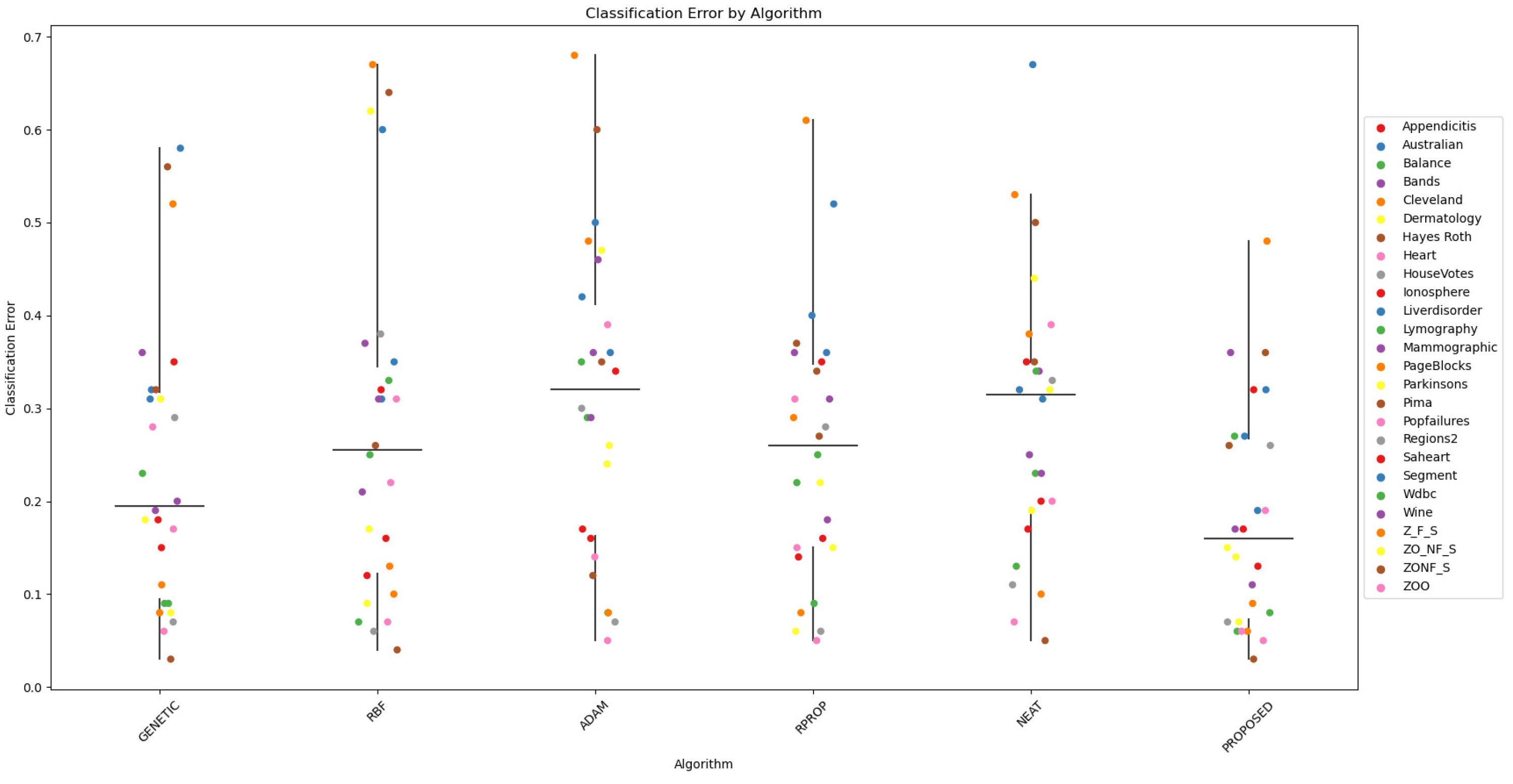
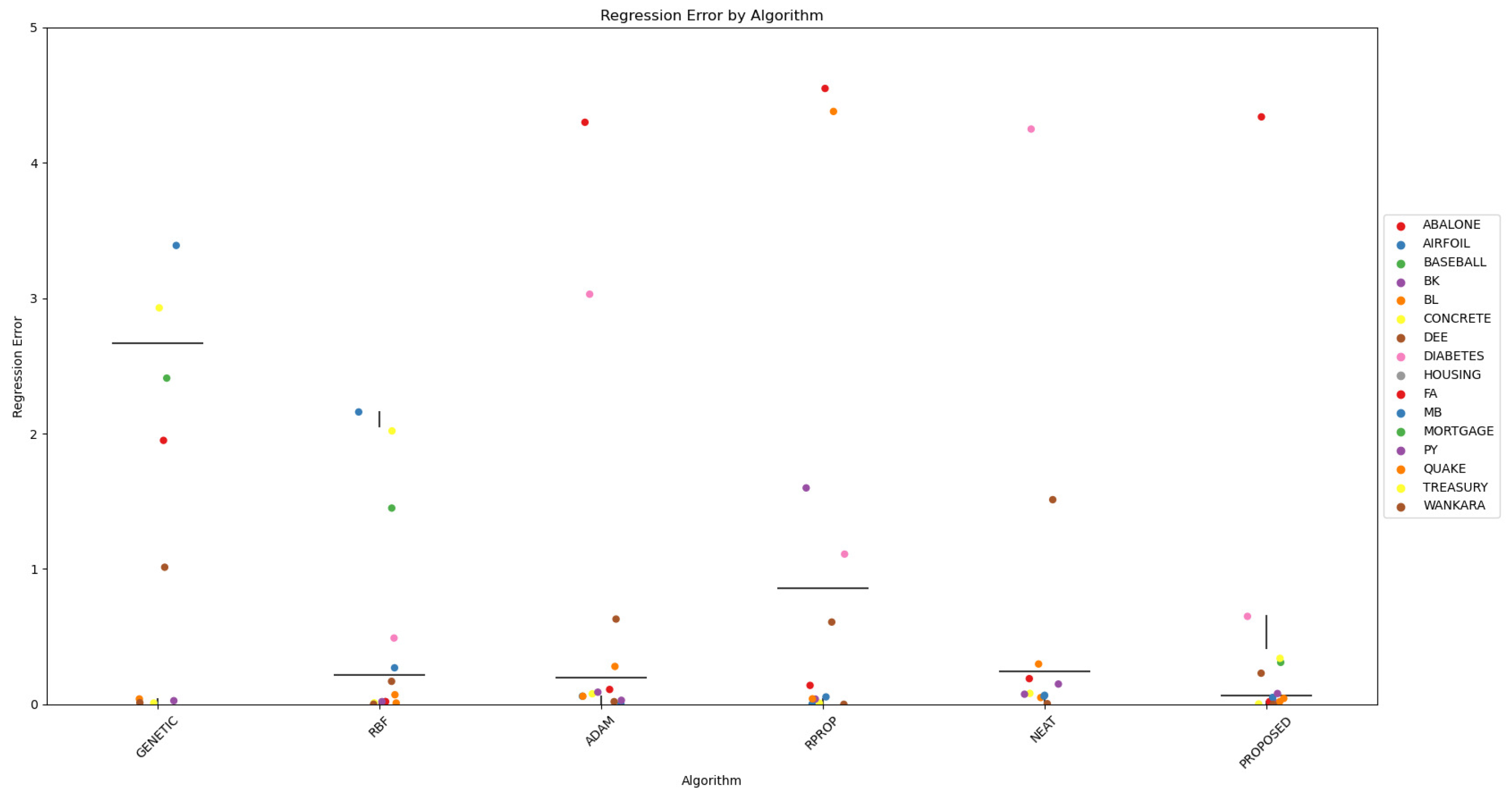
Furthermore, scatter plots that indicate the performance of all mentioned methods are shown in Figure 1 and Figure 2.
In addition, the effectiveness of the usage of the BFGS local search method is measured in an additional experiment, where the local search method for the proposed technique is replaced by the ADAM optimizer. The results for the classification datasets are shown in Table 5 and the corresponding results for the regression datasets in Table 6. In both tables, the column PROPOSED_BFGS denotes the application of the proposed method using the BFGS local search as the procedure of the second phase, and the column PROPOSED_ADAM denotes the incorporation of the ADAM optimizer during the second phase instead of the BFGS.
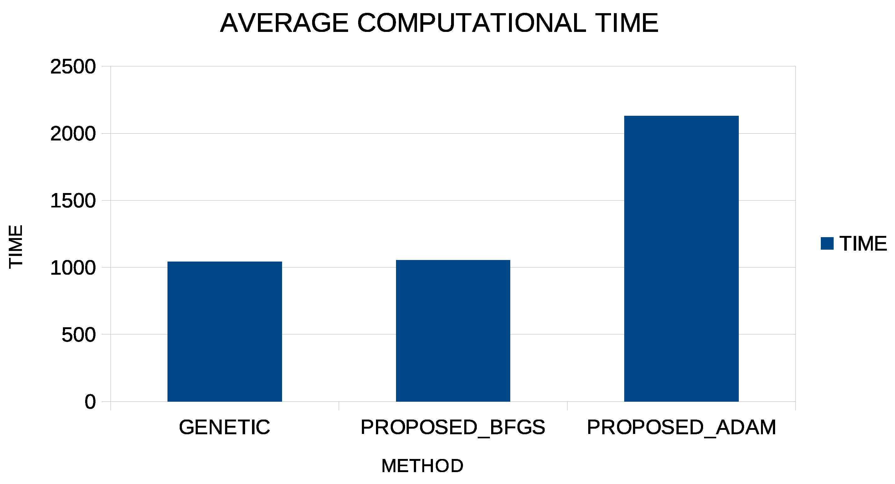
The experimental results demonstrate that the proposed methodology can give excellent results in learning categories or in learning functions, even if the Adam method is used as a local minimization method. However, the Adam method requires a much longer execution time than the BFGS method, and this is shown graphically in Figure 3.
This graph shows the running time for the Abalone dataset, which is a time-consuming problem. The first column shows the execution time for the simple genetic algorithm; the second column shows the execution time for the proposed method using the BFGS local optimization method in the second phase; and the third column shows the execution time for the proposed method using the Adam method in the second stage. Although, as shown in the previous tables, the Adam method can have similar levels of success as the BFGS method, it nevertheless requires significant computing time for its completion.
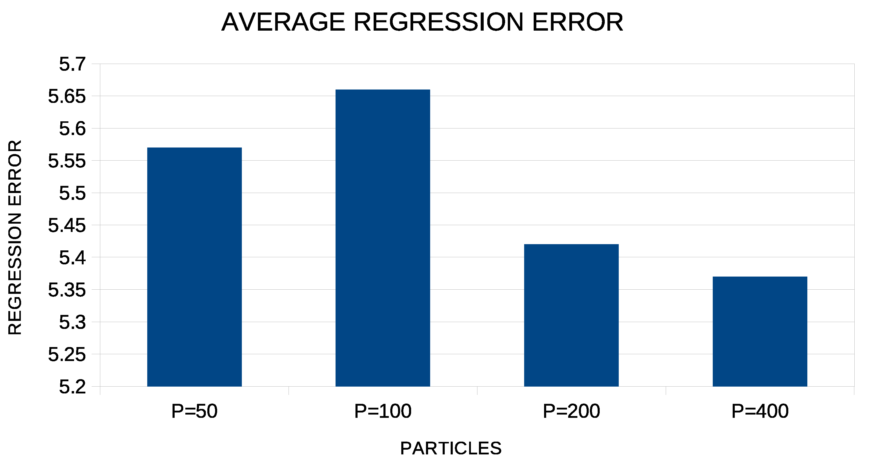
In addition, the average regression error for the proposed method when the number of particles increases from 50 to 400 is graphically outlined in Figure 4.
The proposed technique achieves the best results when the number of particles in the particle swarm optimization exceeds 100. However, the average error is about the same for 200 and 400 particles, and therefore, choosing 200 particles to run experiments appears to be more effective, since it will require less computing time.
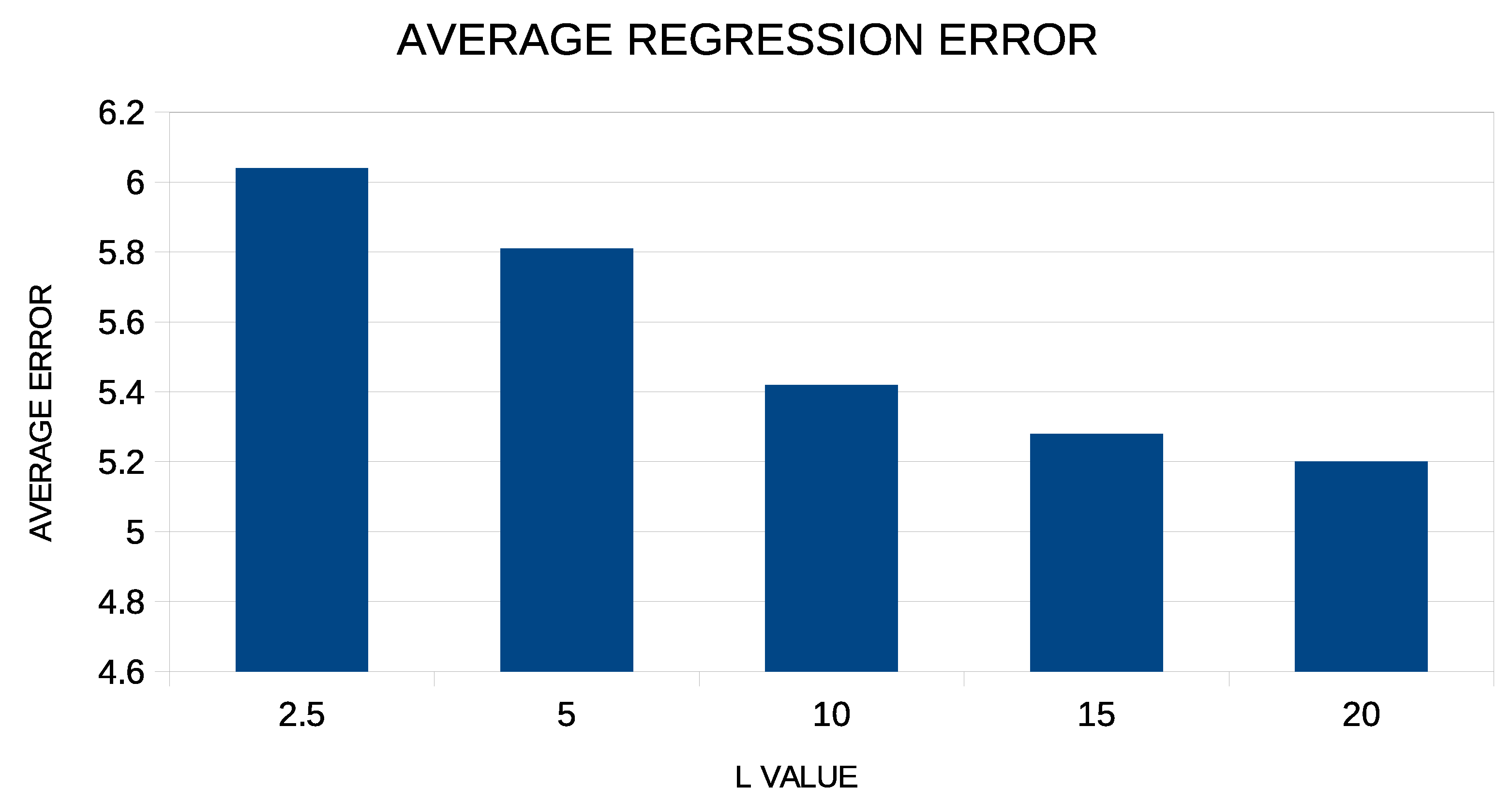
In addition, in order to see if there is a dependence of the results on the critical parameters L and F of the proposed method, a series of additional experiments were carried out in which these parameters were varied. In the first phase, the proposed technique was applied to the regression datasets for different values of the coefficient L varying from 2.5 to 20.0, and the average regression error is graphically shown in Figure 5.
From the experimental results, it is clear that the increase in the value of the coefficient positively affects the performance of the method. However, after the value , this effect decreases drastically. For low values of this coefficient, the parameters of the artificial neural network are limited to low values, and therefore, a lag in the accuracy of the neural network is expected.
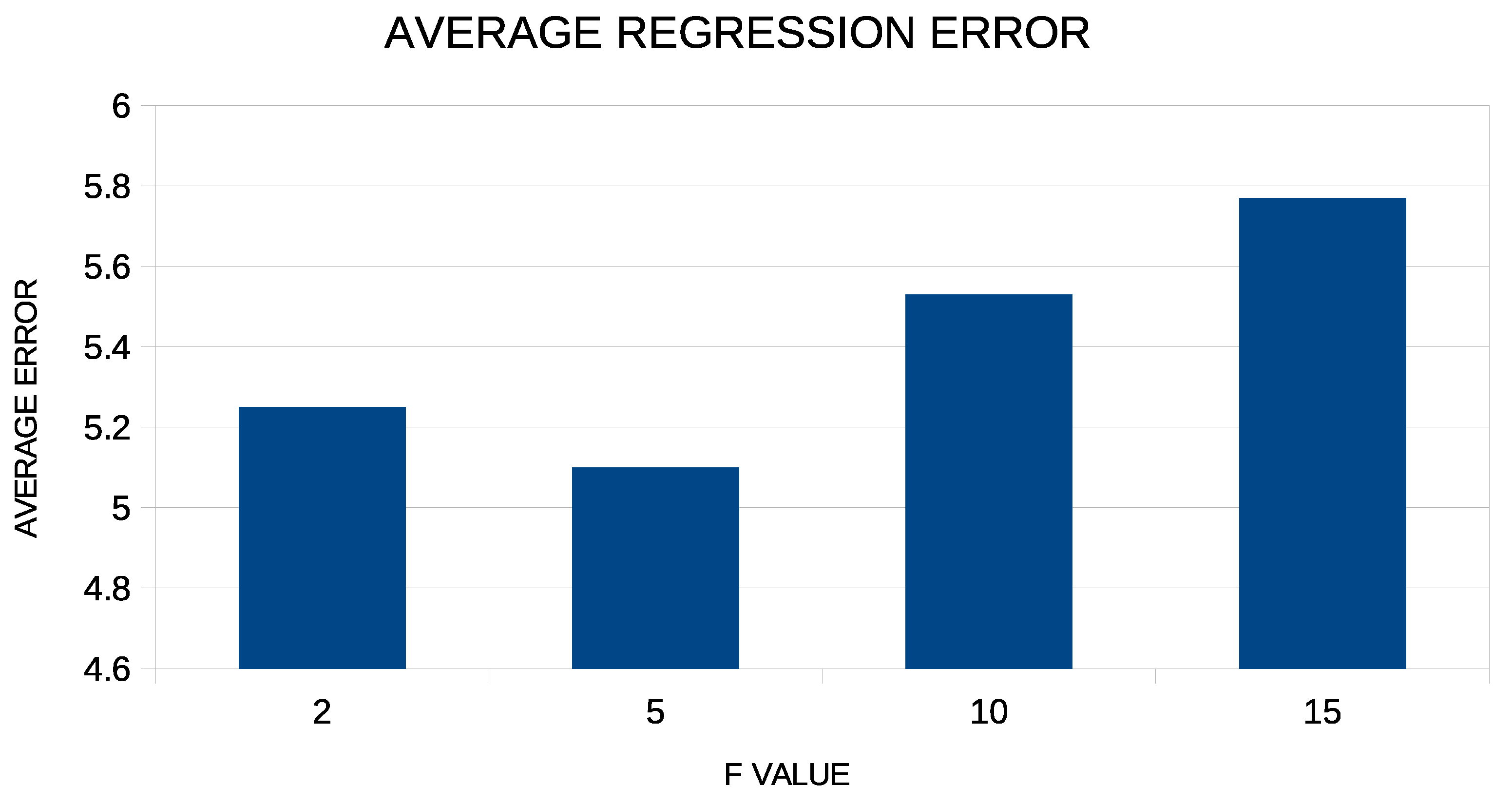
In addition, corresponding experiments were performed with the value of the coefficient F increasing from 2 to 15, and these are graphically illustrated in Figure 6.
For the experiments with the coefficient F, one can see that the gain from any variation of this coefficient is limited, although the lowest values of the average error are achieved when the coefficient has a value close to five.
4. Conclusions
In this paper, a two-stage technique for efficient training of artificial neural networks problems found in many scientific fields was presented. During the first phase, a widely used global optimization technique such as the Particle Swarm Optimization, to which a penalty factor had been added, was used to minimize the training error of the artificial neural network. This penalty factor is incorporated to maintain the effectiveness of the artificial neural network in generalizing to unknown data as well. The calculation of the penalty factor is based on the observation that the artificial neural network can lose its generalization abilities when the input values in the sigmoid activation function exceed some predetermined threshold. After the particle optimization technique is performed in the second phase, the best particle is used both as an initializer of a local optimization method and as a basis for calculating bounds on the parameters of the artificial neural network.
The suggested method was applied to a wide range of classification and regression problems found in the recent literature, and the experimental results were more than encouraging. In addition, when comparing the proposed technique with other widely used methods from the relevant literature, it seems that the proposed technique significantly outperforms them, especially in the case of regression problems. In relevant experiments carried out regarding the sensitivity of the proposed technique on its critical parameters, it was found to be quite robust without large error fluctuations.
Future extensions of the technique may include its application to other network cases such as Radial Basis Function artificial neural networks (RBFs), as well as the use of global optimization methods in the second stage of the proposed technique or even the creation of appropriate termination techniques.
Author Contributions
A.T. and I.G.T. conducted the experiments, employing several datasets and provided the comparative experiments. D.T. and E.K. performed the statistical analysis and prepared the manuscript. All authors have read and agreed to the published version of the manuscript.
Funding
This research received no external funding.
Institutional Review Board Statement
Not applicable.
Informed Consent Statement
Not applicable.
Data Availability Statement
Not applicable.
Acknowledgments
The experiments of this research work were performed at the high performance computing system established at Knowledge and Intelligent Computing Laboratory, Department of Informatics and Telecommunications, University of Ioannina, acquired with the project “Educational Laboratory equipment of TEI of Epirus” with MIS 5007094 funded by the Operational Programme “Epirus” 2014–2020, by ERDF and national funds.
Conflicts of Interest
The authors declare no conflict of interest.
Sample Availability
Not applicable.
References
- Bishop, C. Neural Networks for Pattern Recognition; Oxford University Press: Oxford, UK, 1995. [Google Scholar]
- Cybenko, G. Approximation by superpositions of a sigmoidal function. Math. Control. Signals Syst. 1989, 2, 303–314. [Google Scholar] [CrossRef]
- Baldi, P.; Cranmer, K.; Faucett, T.; Sadowski, P.; Whiteson, D. Parameterized neural networks for high-energy physics. Eur. Phys. J. C 2016, 76, 1–7. [Google Scholar] [CrossRef]
- Valdas, J.J.; Bonham-Carter, G. Time dependent neural network models for detecting changes of state in complex processes: Applications in earth sciences and astronomy. Neural Netw. 2006, 19, 196–207. [Google Scholar] [CrossRef]
- Carleo, G. Solving the quantum many-body problem with artificial neural networks. Science 2017, 355, 602–606. [Google Scholar] [CrossRef] [PubMed]
- Shen, L.; Wu, J.; Yang, W. Multiscale Quantum Mechanics/Molecular Mechanics Simulations with Neural Networks. J. Chem. Theory Comput. 2016, 12, 4934–4946. [Google Scholar] [CrossRef] [PubMed]
- Manzhos, S.; Dawes, R.; Carrington, T. Neural network-based approaches for building high dimensional and quantum dynamics-friendly potential energy surfaces. Int. J. Quantum Chem. 2015, 115, 1012–1020. [Google Scholar] [CrossRef]
- Wei, J.N.; Duvenaud, D.; Aspuru-Guzik, A. Neural Networks for the Prediction of Organic Chemistry Reactions. ACS Cent. Sci. 2016, 2, 725–732. [Google Scholar] [CrossRef]
- Baskin, I.I.; Winkler, D.; Tetko, I.V. A renaissance of neural networks in drug discovery. Expert Opin. Drug Discov. 2016, 11, 785–795. [Google Scholar] [CrossRef]
- Bartzatt, R. Prediction of Novel Anti-Ebola Virus Compounds Utilizing Artificial Neural Network (ANN). Chem. Fac. 2018, 49, 16–34. [Google Scholar]
- Falat, L.; Pancikova, L. Quantitative Modelling in Economics with Advanced Artificial Neural Networks. Procedia Econ. Financ. 2015, 34, 194–201. [Google Scholar] [CrossRef]
- Namazi, M.; Shokrolahi, A.; Maharluie, M.S. Detecting and ranking cash flow risk factors via artificial neural networks technique. J. Bus. Res. 2016, 69, 1801–1806. [Google Scholar] [CrossRef]
- Tkacz, G. Neural network forecasting of Canadian GDP growth. Int. J. Forecast. 2001, 17, 57–69. [Google Scholar] [CrossRef]
- Shirvany, Y.; Hayati, M.; Moradian, R. Multilayer perceptron neural networks with novel unsupervised training method for numerical solution of the partial differential equations. Appl. Soft Comput. 2009, 9, 20–29. [Google Scholar] [CrossRef]
- Malek, A.; Beidokhti, R.S. Numerical solution for high order differential equations using a hybrid neural network—Optimization method. Appl. Math. Comput. 2006, 183, 260–271. [Google Scholar] [CrossRef]
- Topuz, A. Predicting moisture content of agricultural products using artificial neural networks. Adv. Eng. 2010, 41, 464–470. [Google Scholar] [CrossRef]
- Escamilla-García, A.; Soto-Zarazúa, G.M.; Toledano-Ayala, M.; Rivas-Araiza, E.; Gastélum-Barrios, A. Applications of Artificial Neural Networks in Greenhouse Technology and Overview for Smart Agriculture Development. Appl. Sci. 2020, 10, 3835. [Google Scholar] [CrossRef]
- Boughrara, H.; Chtourou, M.; Amar, C.B.; Chen, L. Facial expression recognition based on a mlp neural network using constructive training algorithm. Multimed Tools Appl. 2016, 75, 709–731. [Google Scholar] [CrossRef]
- Liu, H.; Tian, H.Q.; Li, Y.F.; Zhang, L. Comparison of four Adaboost algorithm based artificial neural networks in wind speed predictions. Energy Convers. Manag. 2015, 92, 67–81. [Google Scholar] [CrossRef]
- Szoplik, J. Forecasting of natural gas consumption with artificial neural networks. Energy 2015, 85, 208–220. [Google Scholar] [CrossRef]
- Bahram, H.; Navimipour, N.J. Intrusion detection for cloud computing using neural networks and artificial bee colony optimization algorithm. ICT Express 2019, 5, 56–59. [Google Scholar]
- Rumelhart, D.E.; Hinton, G.E.; Williams, R.J. Learning representations by back-propagating errors. Nature 1986, 323, 533–536. [Google Scholar] [CrossRef]
- Chen, T.; Zhong, S. Privacy-Preserving Backpropagation Neural Network Learning. IEEE Trans. Neural Netw. 2009, 20, 1554–1564. [Google Scholar] [CrossRef] [PubMed]
- Riedmiller, M.; Braun, H. A Direct Adaptive Method for Faster Backpropagation Learning: The RPROP algorithm. In Proceedings of the IEEE International Conference on Neural Networks, San Francisco, CA, USA, 28 March–1 April 1993; pp. 586–591. [Google Scholar]
- Pajchrowski, T.; Zawirski, K.; Nowopolski, K. Neural Speed Controller Trained Online by Means of Modified RPROP Algorithm. IEEE Trans. Ind. Inform. 2015, 11, 560–568. [Google Scholar] [CrossRef]
- Hermanto, R.P.S.; Nugroho, A. Waiting-Time Estimation in Bank Customer Queues using RPROP Neural Networks. Procedia Comput. Sci. 2018, 135, 35–42. [Google Scholar] [CrossRef]
- Robitaille, B.; Marcos, B.; Veillette, M.; Payre, G. Modified quasi-Newton methods for training neural networks. Comput. Chem. Eng. 1996, 20, 1133–1140. [Google Scholar] [CrossRef]
- Liu, Q.; Liu, J.; Sang, R.; Li, J.; Zhang, T.; Zhang, Q. Fast Neural Network Training on FPGA Using Quasi-Newton Optimization Method. IEEE Trans. Very Large Scale Integr. (VLSI) Syst. 2018, 26, 1575–1579. [Google Scholar] [CrossRef]
- Yamazaki, A.; de Souto, M.C.P. Optimization of neural network weights and architectures for odor recognition using simulated annealing. In Proceedings of the 2002 International Joint Conference on Neural Networks, IJCNN’02 1, Honolulu, HI, USA, 12–17 May 2002; pp. 547–552. [Google Scholar]
- Da, Y.; Xiurun, G. An improved PSO-based ANN with simulated annealing technique. Neurocomputing 2005, 63, 527–533. [Google Scholar] [CrossRef]
- Leung, F.H.F.; Lam, H.K.; Ling, S.H.; Tam, P.K.S. Tuning of the structure and parameters of a neural network using an improved genetic algorithm. IEEE Trans. Neural Netw. 2003, 14, 79–88. [Google Scholar] [CrossRef]
- Yao, X. Evolving artificial neural networks. Proc. IEEE 1999, 87, 1423–1447. [Google Scholar]
- Zhang, C.; Shao, H.; Li, Y. Particle swarm optimisation for evolving artificial neural network. In Proceedings of the IEEE International Conference on Systems, Man, and Cybernetics, Nashville, TN, USA, 8–11 October 2000; pp. 2487–2490. [Google Scholar]
- Yu, J.; Wang, S.; Xi, L. Evolving artificial neural networks using an improved PSO and DPSO. Neurocomputing 2008, 71, 1054–1060. [Google Scholar] [CrossRef]
- Ilonen, J.; Kamarainen, J.K.; Lampinen, J. Differential Evolution Training Algorithm for Feed-Forward Neural Networks. Neural Process. Lett. 2003, 17, 93–105. [Google Scholar] [CrossRef]
- Rocha, M.; Cortez, P.; Neves, J. Evolution of neural networks for classification and regression. Neurocomputing 2007, 70, 2809–2816. [Google Scholar] [CrossRef]
- Aljarah, I.; Faris, H.; Mirjalili, S. Optimizing connection weights in neural networks using the whale optimization algorithm. Soft Comput. 2018, 22, 1–15. [Google Scholar] [CrossRef]
- Jalali, S.M.J.; Ahmadian, S.; Kebria, P.M.; Khosravi, A.; Lim, C.P.; Nahavandi, S. Evolving Artificial Neural Networks Using Butterfly Optimization Algorithm for Data Classification. In Neural Information Processing. ICONIP 2019; Lecture Notes in Computer Science; Gedeon, T., Wong, K., Lee, M., Eds.; Springer: Cham, Switzerland, 2019; Volume 11953. [Google Scholar]
- Ivanova, I.; Kubat, M. Initialization of neural networks by means of decision trees. Knowl. Based Syst. 1995, 8, 333–344. [Google Scholar] [CrossRef]
- Yam, J.Y.F.; Chow, T.W.S. A weight initialization method for improving training speed in feedforward neural network. Neurocomputing 2000, 30, 219–232. [Google Scholar] [CrossRef]
- Itano, F.; de Abreu de Sousa, M.A.; Del-Moral-Hernandez, E. Extending MLP ANN hyper-parameters Optimization by using Genetic Algorithm. In Proceedings of the 2018 International Joint Conference on Neural Networks (IJCNN), Rio de Janeiro, Brazil, 8–13 July 2018; Volume 2018, pp. 1–8. [Google Scholar]
- Chumachenko, K.; Iosifidis, A.; Gabbouj, M. Feedforward neural networks initialization based on discriminant learning. Neural Netw. 2022, 146, 220–229. [Google Scholar] [CrossRef] [PubMed]
- Setiono, R. Feedforward Neural Network Construction Using Cross Validation. Neural Comput. 2001, 13, 2865–2877. [Google Scholar] [CrossRef]
- O’Neill, M.; Ryan, C. Grammatical evolution. IEEE Trans. Evol. Comput. 2001, 5, 349–358. [Google Scholar] [CrossRef]
- Tsoulos, I.G.; Gavrilis, D.; Glavas, E. Neural network construction and training using grammatical evolution. Neurocomputing 2008, 72, 269–277. [Google Scholar] [CrossRef]
- Kim, K.J.; Cho, S.B. Evolved neural networks based on cellular automata for sensory-motor controller. Neurocomputing 2006, 69, 2193–2207. [Google Scholar] [CrossRef]
- Martínez-Zarzuela, M.; Pernas, F.J.D.; Higuera, J.F.D.; Rodríguez, M.A. Fuzzy ART Neural Network Parallel Computing on the GPU. In Computational and Ambient Intelligence. IWANN 2007; Lecture Notes in Computer Science; Sandoval, F., Prieto, A., Cabestany, J., Graña, M., Eds.; Springer: Berlin/Heidelberg, Germany, 2007; Volume 4507. [Google Scholar]
- Huqqani, A.A.; Schikuta, E.; Chen, S.Y.P. Multicore and GPU Parallelization of Neural Networks for Face Recognition. Procedia Comput. Sci. 2013, 18, 349–358. [Google Scholar] [CrossRef]
- Nowlan, S.J.; Hinton, G.E. Simplifying neural networks by soft weight sharing. Neural Comput. 1992, 4, 473–493. [Google Scholar] [CrossRef]
- Kim, J.K.; Lee, M.Y.; Kim, J.Y.; Kim, B.J.; Lee, J.H. An efficient pruning and weight sharing method for neural network. In Proceedings of the 2016 IEEE International Conference on Consumer Electronics-Asia (ICCE-Asia), Seoul, Republic of Korea, 26–28 October 2016; pp. 1–2. [Google Scholar]
- Hanson, S.J.; Pratt, L.Y. Comparing biases for minimal network construction with back propagation, In Advances in Neural Information Processing Systems; Touretzky, D.S., Ed.; Morgan Kaufmann: San Mateo, CA, USA, 1989; Volume 1, pp. 177–185. [Google Scholar]
- Mozer, M.C.; Smolensky, P. Skeletonization: A technique for trimming the fat from a network via relevance assesment. In Advances in Neural Processing Systems; Touretzky, D.S., Ed.; Morgan Kaufmann: San Mateo CA, USA, 1989; Volume 1, pp. 107–115. [Google Scholar]
- Augasta, M.; Kathirvalavakumar, T. Pruning algorithms of neural networks—A comparative study. Cent. Eur. Comput. Sci. 2003, 3, 105–115. [Google Scholar] [CrossRef]
- Srivastava, N.; Hinton, G.; Krizhevsky, A.; Sutskever, I.; Salakhutdinov, R. Dropout: A simple way to prevent neural networks from overfitting. J. Mach. Learn. Res. 2014, 15, 1929–1958. [Google Scholar]
- Iosifidis, A.; Tefas, A.; Pitas, I. DropELM: Fast neural network regularization with Dropout and DropConnect. Neurocomputing 2015, 162, 57–66. [Google Scholar] [CrossRef]
- Gupta, A.; Lam, S.M. Weight decay backpropagation for noisy data. Neural Netw. 1998, 11, 1127–1138. [Google Scholar] [CrossRef] [PubMed]
- Carvalho, M.; Ludermir, T.B. Particle Swarm Optimization of Feed-Forward Neural Networks with Weight Decay. In Proceedings of the 2006 Sixth International Conference on Hybrid Intelligent Systems (HIS’06), Rio de Janeiro, Brazil, 13–15 December 2006; p. 5. [Google Scholar]
- Treadgold, N.K.; Gedeon, T.D. Simulated annealing and weight decay in adaptive learning: The SARPROP algorithm. IEEE Trans. Neural Netw. 1998, 9, 662–668. [Google Scholar] [CrossRef]
- Shahjahan, M.D.; Kazuyuki, M. Neural network training algorithm with possitive correlation. IEEE Trans. Inf. Syst. 2005, 88, 2399–2409. [Google Scholar] [CrossRef]
- Geman, S.; Bienenstock, E.; Doursat, R. Neural networks and the bias/variance dilemma. Neural Comput. 1992, 4, 1–58. [Google Scholar] [CrossRef]
- Hawkins, D.M. The Problem of Overfitting. J. Chem. Inf. Comput. Sci. 2004, 44, 1–12. [Google Scholar] [CrossRef]
- Marini, F.; Walczak, B. Particle swarm optimization (PSO). A tutorial. Chemom. Intell. Lab. Syst. 2015, 149, 153–165. [Google Scholar] [CrossRef]
- de Moura Meneses, A.A.; Machado, M.D.; Schirru, M.R. Particle Swarm Optimization applied to the nuclear reload problem of a Pressurized Water Reactor. Progress Nucl. Energy 2009, 51, 319–326. [Google Scholar] [CrossRef]
- Shaw, R.; Srivastava, S. Particle swarm optimization: A new tool to invert geophysical data. Geophysics 2007, 72, F75–F83. [Google Scholar] [CrossRef]
- Ourique, C.O.; Biscaia, E.C.; Pinto, J.C. The use of particle swarm optimization for dynamical analysis in chemical processes. Comput. Chem. Eng. 2002, 26, 1783–1793. [Google Scholar] [CrossRef]
- Fang, H.; Zhou, J.; Wang, Z.; Qiu, Z.; Sun, Y.; Lin, Y.; Chen, K.; Zhou, X.; Pan, M. Hybrid method integrating machine learning and particle swarm optimization for smart chemical process operations. Front. Chem. Sci. Eng. 2022, 16, 274–287. [Google Scholar] [CrossRef]
- Wachowiak, M.P.; Smolikova, R.; Zheng, Y.; Zurada, J.M.; Elmaghraby, A.S. An approach to multimodal biomedical image registration utilizing particle swarm optimization. IEEE Trans. Evol. Comput. 2004, 8, 289–301. [Google Scholar] [CrossRef]
- Marinaki, Y.M.M.; Dounias, G. Particle swarm optimization for pap-smear diagnosis. Expert Syst. Appl. 2008, 35, 1645–1656. [Google Scholar] [CrossRef]
- Park, J.-B.; Jeong, Y.-W.; Shin, J.-R.; Lee, K.Y. An Improved Particle Swarm Optimization for Nonconvex Economic Dispatch Problems. IEEE Trans. Power Syst. 2010, 25, 156–162. [Google Scholar] [CrossRef]
- Hwang, J.T.G.; Ding, A.A. Prediction Intervals for Artificial Neural Networks. J. Am. Stat. 1997, 92, 748–757. [Google Scholar] [CrossRef]
- Kasiviswanathan, K.S.; Cibin, R.; Sudheer, K.P.; Chaubey, I. Constructing prediction interval for artificial neural network rainfall runoff models based on ensemble simulations. J. Hydrol. 2013, 499, 275–288. [Google Scholar] [CrossRef]
- Sodhi, S.S.; Chandra, P. Interval based Weight Initialization Method for Sigmoidal Feedforward Artificial Neural Networks. AASRI Procedia 2014, 6, 19–25. [Google Scholar] [CrossRef]
- Narkhede, M.V.; Bartakke, P.P.; Sutaone, M.S. A review on weight initialization strategies for neural networks. Artif. Intell. Rev. 2022, 55, 291–322. [Google Scholar] [CrossRef]
- Kennedy, J.; Eberhart, R. Particle swarm optimization. In Proceedings of the ICNN’95—International Conference on Neural Networks, Perth, Australia, 27 November–1 December 1995; Volume 4, pp. 1942–1948. [Google Scholar] [CrossRef]
- Eberhart, R.C.; Shi, Y.H. Tracking and optimizing dynamic systems with particle swarms. In Proceedings of the 2001 Congress on Evolutionary Computation (IEEE Cat. No.01TH8546), Seoul, Republic of Korea, 27–30 May 2001. [Google Scholar]
- Shi, Y.H.; Eberhart, R.C. Empirical study of particle swarm optimization. In Proceedings of the 1999 Congress on Evolutionary Computation-CEC99 (Cat. No. 99TH8406), Washington, DC, USA, 6–9 July 1999. [Google Scholar]
- Shi, Y.H.; Eberhart, R.C. Experimental study of particle swarm optimization. In Proceedings of the SCI2000 Conference, Orlando, FL, USA, 30 April–2 May 2000. [Google Scholar]
- Powell, M.J.D. A Tolerant Algorithm for Linearly Constrained Optimization Calculations. Math. Program. 1989, 45, 547–566. [Google Scholar] [CrossRef]
- Fletcher, R. A new approach to variable metric algorithms. Comput. J. 1970, 13, 317–322. [Google Scholar] [CrossRef]
- Alcalá-Fdez, J.; Fernandez, A.; Luengo, J.; Derrac, J.; García, S.; Sánchez, L.; Herrera, F. KEEL Data-Mining Software Tool: Data Set Repository, Integration of Algorithms and Experimental Analysis Framework. J. Mult. Valued Log. Soft Comput. 2011, 17, 255–287. [Google Scholar]
- Weiss, S.M.; Kulikowski, C.A. Computer Systems That Learn: Classification and Prediction Methods from Statistics, Neural Nets, Machine Learning, and Expert Systems; Morgan Kaufmann Publishers Inc.: San Mateo CA, USA, 1991. [Google Scholar]
- Quinlan, J.R. Simplifying Decision Trees. Int. Man Mach. Stud. 1987, 27, 221–234. [Google Scholar] [CrossRef]
- Shultz, T.; Mareschal, D. Schmidt, Modeling Cognitive Development on Balance Scale Phenomena. Mach. Learn. 1994, 16, 59–88. [Google Scholar] [CrossRef]
- Zhou, Z.H. NeC4.5: Neural ensemble based C4.5. IEEE Trans. Knowl. Data Eng. 2004, 16, 770–773. [Google Scholar] [CrossRef]
- Setiono, R.; Leow, W.K. FERNN: An Algorithm for Fast Extraction of Rules from Neural Networks. Appl. Intell. 2000, 12, 15–25. [Google Scholar] [CrossRef]
- Demiroz, G.; Govenir, H.A.; Ilter, N. Learning Differential Diagnosis of Eryhemato-Squamous Diseases using Voting Feature Intervals. Artif. Intell. Med. 1998, 13, 147–165. [Google Scholar]
- Kononenko, I.; Šimec, E.; Robnik-Šikonja, M. Overcoming the Myopia of Inductive Learning Algorithms with RELIEFF. Appl. Intell. 1997, 7, 39–55. [Google Scholar] [CrossRef]
- Hayes-Roth, B.; Hayes-Roth, F. Concept learning and the recognition and classification of exemplars. J. Verbal Learning Verbal Behav. 1977, 16, 321–338. [Google Scholar] [CrossRef]
- French, R.M.; Chater, N. Using noise to compute error surfaces in connectionist networks: A novel means of reducing catastrophic forgetting. Neural Comput. 2002, 14, 1755–1769. [Google Scholar] [CrossRef]
- Dy, J.G.; Brodley, C.E. Feature Selection for Unsupervised Learning. J. Mach. Learn. Res. 2004, 5, 45–889. [Google Scholar]
- Perantonis, S.J.; Virvilis, V. Input Feature Extraction for Multilayered Perceptrons Using Supervised Principal Component Analysis. Neural Process. Lett. 1999, 10, 243–252. [Google Scholar] [CrossRef]
- Garcke, J.; Griebel, M. Classification with sparse grids using simplicial basis functions. Intell. Data Anal. 2002, 6, 483–502. [Google Scholar] [CrossRef]
- Elter, M.; Schulz-Wendtland, R.; Wittenberg, T. The prediction of breast cancer biopsy outcomes using two CAD approaches that both emphasize an intelligible decision process. Med. Phys. 2007, 34, 4164–4172. [Google Scholar] [CrossRef]
- Esposito, F.F.; Malerba, D.; Semeraro, G. Multistrategy Learning for Document Recognition. Appl. Artif. Intell. 1994, 8, 33–84. [Google Scholar] [CrossRef]
- Little, M.A.; McSharry, P.E.; Hunter, E.J.; Spielman, J.; Ramig, L.O. Suitability of dysphonia measurements for telemonitoring of Parkinson’s disease. IEEE Trans. Biomed. Eng. 2009, 56, 1015–1022. [Google Scholar] [CrossRef] [PubMed]
- Smith, J.W.; Everhart, J.E.; Dickson, W.C.; Knowler, W.C.; Johannes, R.S. Using the ADAP learning algorithm to forecast the onset of diabetes mellitus. In Proceedings of the Symposium on Computer Applications and Medical Care IEEE Computer Society Press, Minneapolis, MN, USA, 8–10 June 1988; pp. 261–265. [Google Scholar]
- Lucas, D.D.; Klein, R.; Tannahill, J.; Ivanova, D.; Brandon, S.; Domyancic, D.; Zhang, Y. Failure analysis of parameter-induced simulation crashes in climate models. Geosci. Model Dev. 2013, 6, 1157–1171. [Google Scholar] [CrossRef]
- Giannakeas, N.; Tsipouras, M.G.; Tzallas, A.T.; Kyriakidi, K.; Tsianou, Z.E.; Manousou, P.; Hall, A.; Karvounis, E.C.; Tsianos, V.; Tsianos, E. A clustering based method for collagen proportional area extraction in liver biopsy images. In Proceedings of the Annual International Conference of the IEEE Engineering in Medicine and Biology Society, EMBS, Milan, Italy, 25–29 August 2015; pp. 3097–3100. [Google Scholar]
- Hastie, T.; Tibshirani, R. Non-parametric logistic and proportional odds regression. JRSS-C (Appl. Stat.) 1987, 36, 260–276. [Google Scholar] [CrossRef]
- Dash, M.; Liu, H.; Scheuermann, P.; Tan, K.L. Fast hierarchical clustering and its validation. Data Knowl. Eng. 2003, 44, 109–138. [Google Scholar] [CrossRef]
- Wolberg, W.H.; Mangasarian, O.L. Multisurface method of pattern separation for medical diagnosis applied to breast cytology. Proc. Natl. Acad. Sci. USA 1990, 87, 9193–9196. [Google Scholar] [CrossRef] [PubMed]
- Raymer, M.; Doom, T.E.; Kuhn, L.A.; Punch, W.F. Knowledge discovery in medical and biological datasets using a hybrid Bayes classifier/evolutionary algorithm. IEEE Trans. Syst. Man Cybern. Part B 2003, 33, 802–813. [Google Scholar] [CrossRef]
- Zhong, P.; Fukushima, M. Regularized nonsmooth Newton method for multi-class support vector machines. Optim. Methods Softw. 2007, 22, 225–236. [Google Scholar] [CrossRef]
- Koivisto, M.; Sood, K. Exact Bayesian Structure Discovery in Bayesian Networks. J. Mach. Learn. Res. 2004, 5, 549–573. [Google Scholar]
- Nash, W.J.; Sellers, T.L.; Talbot, S.R.; Cawthor, A.J.; Ford, W.B. The Population Biology of Abalone (_Haliotis_ species) in Tasmania. I. Blacklip Abalone (_H. rubra_) from the North Coast and Islands of Bass Strait, Sea Fisheries Division; Technical Report No. 48 (ISSN 1034-3288); Department of Primary Industry and Fisheries, Tasmania: Hobart, Australia, 1994. [Google Scholar]
- Brooks, T.F.; Pope, D.S.; Marcolini, A.M. Airfoil Self-Noise and Prediction; Technical Report, NASA RP-1218; National Aeronautics and Space Administration: Washington, DC, USA, 1989. [Google Scholar]
- Simonoff, J.S. Smooting Methods in Statistics; Springer: Berlin/Heidelberg, Germany, 1996. [Google Scholar]
- Yeh, I.C. Modeling of strength of high performance concrete using artificial neural networks. Cem. Concr. Res. 1998, 28, 1797–1808. [Google Scholar] [CrossRef]
- Harrison, D.; Rubinfeld, D.L. Hedonic prices and the demand for clean ai. J. Environ. Econ. Manag. 1978, 5, 81–102. [Google Scholar] [CrossRef]
- King, R.D.; Muggleton, S.; Lewis, R.A.; Sternberg, M.J. Drug design by machine learning: The use of inductive logic programming to model the structure-activity relationships of trimethoprim analogues binding to dihydrofolate reductase. Proc. Nat. Acad. Sci. USA 1992, 89, 11322–11326. [Google Scholar] [CrossRef] [PubMed]
- Park, J.; Sandberg, I.W. Universal Approximation Using Radial-Basis-Function Networks. Neural Comput. 1991, 3, 246–257. [Google Scholar] [CrossRef]
- Kingma, D.P.; Ba, J.L. ADAM: A method for stochastic optimization. In Proceedings of the 3rd International Conference on Learning Representations (ICLR 2015), San Diego, CA, USA, 7–9 May 2015; pp. 1–15. [Google Scholar]
- Klima, G. Fast Compressed Neural Networks. Available online: http://fcnn.sourceforge.net/ (accessed on 14 April 2023).
- Stanley, K.O.; Miikkulainen, R. Evolving Neural Networks through Augmenting Topologies. Evol. Comput. 2002, 10, 99–127. [Google Scholar] [CrossRef] [PubMed]
Figure 1.
The scatter plot provides a clear overview of the performance of the proposed algorithm compared to the other six algorithms across the 26 datasets. It allows for visual identification of patterns, trends, and potential outliers in the classification errors. The plot serves as a concise visual summary of the comparative performance of the algorithms, providing insights into the effectiveness of the proposed algorithm in relation to the other algorithms in a variety of datasets.

Figure 2.
The scatter plot visually represents the performance of the regression classification algorithms in terms of classification errors. Each point on the plot represents the regression error of a particular algorithm in a specific dataset. The x-axis represents the regression algorithms, while the y-axis represents the regression error. Different datasets are denoted by different colors for clarity.

Figure 3.
Average execution time for the Abalone dataset for three different methods: The simplegGenetic method, the proposed method with the incorporation of BFGS, and the proposed method with the usage of the Adam optimizer during the second phase of execution.
Figure 3.
Average execution time for the Abalone dataset for three different methods: The simplegGenetic method, the proposed method with the incorporation of BFGS, and the proposed method with the usage of the Adam optimizer during the second phase of execution.

Figure 4.
Average regression error for the proposed method using different numbers of particles in each experiment.
Figure 4.
Average regression error for the proposed method using different numbers of particles in each experiment.

Figure 5.
Experiments with the L parameter for the regression datasets.

Figure 6.
Experiments with the value of parameter F for the regression datasets.


Table 1.
This table presents the values of the parameters used during the execution of the experiments.
Table 1.
This table presents the values of the parameters used during the execution of the experiments.
| Parameter | Meaning | Value |
|---|---|---|
| m | Number of particles or chromosomes | 200 |
| Maximum number of iterations | 200 | |
| Minimum value for inertia | 0.4 | |
| Maximum value for inertia | 0.9 | |
| H | Number of weights | 10 |
| Penalty factor | 100.0 | |
| L | The limit for the function | 10.0 |
| F | The margin factor | 5.0 |
Table 2.
Average classification error for the classification datasets for all mentioned methods.
| Dataset | Nclass | Genetic | RBF | ADAM | RPROP | NEAT | Proposed |
|---|---|---|---|---|---|---|---|
| Appendicitis | 2 | 18.10% | 12.23% | 16.50% | 16.30% | 17.20% | 16.97% |
| Australian | 2 | 32.21% | 34.89% | 35.65% | 36.12% | 31.98% | 26.96% |
| Balance | 3 | 8.97% | 33.42% | 7.87% | 8.81% | 23.14% | 7.52% |
| Bands | 2 | 35.75% | 37.22% | 36.25% | 36.32% | 34.30% | 35.77% |
| Cleveland | 5 | 51.60% | 67.10% | 67.55% | 61.41% | 53.44% | 48.40% |
| Dermatology | 6 | 30.58% | 62.34% | 26.14% | 15.12% | 32.43% | 14.30% |
| Hayes Roth | 3 | 56.18% | 64.36% | 59.70% | 37.46% | 50.15% | 36.33% |
| Heart | 2 | 28.34% | 31.20% | 38.53% | 30.51% | 39.27% | 18.99% |
| HouseVotes | 2 | 6.62% | 6.13% | 7.48% | 6.04% | 10.89% | 7.10% |
| Ionosphere | 2 | 15.14% | 16.22% | 16.64% | 13.65% | 19.67% | 13.15% |
| Liverdisorder | 2 | 31.11% | 30.84% | 41.53% | 40.26% | 30.67% | 32.07% |
| Lymography | 4 | 23.26% | 25.31% | 29.26% | 24.67% | 33.70% | 27.05% |
| Mammographic | 2 | 19.88% | 21.38% | 46.25% | 18.46% | 22.85% | 17.37% |
| PageBlocks | 5 | 8.06% | 10.09% | 7.93% | 7.82% | 10.22% | 6.47% |
| Parkinsons | 2 | 18.05% | 17.42% | 24.06% | 22.28% | 18.56% | 14.60% |
| Pima | 2 | 32.19% | 25.78% | 34.85% | 34.27% | 34.51% | 26.34% |
| Popfailures | 2 | 5.94% | 7.04% | 5.18% | 4.81% | 7.05% | 5.27% |
| Regions2 | 5 | 29.39% | 38.29% | 29.85% | 27.53% | 33.23% | 26.29% |
| Saheart | 2 | 34.86% | 32.19% | 34.04% | 34.90% | 34.51% | 32.49% |
| Segment | 7 | 57.72% | 59.68% | 49.75% | 52.14% | 66.72% | 18.99% |
| Wdbc | 2 | 8.56% | 7.27% | 35.35% | 21.57% | 12.88% | 6.01% |
| Wine | 3 | 19.20% | 31.41% | 29.40% | 30.73% | 25.43% | 10.92% |
| Z_F_S | 3 | 10.73% | 13.16% | 47.81% | 29.28% | 38.41% | 8.55% |
| ZO_NF_S | 3 | 8.41% | 9.02% | 47.43% | 6.43% | 43.75% | 7.11% |
| ZONF_S | 2 | 2.60% | 4.03% | 11.99% | 27.27% | 5.44% | 2.61% |
| ZOO | 7 | 16.67% | 21.93% | 14.13% | 15.47% | 20.27% | 5.80% |
| AVERAGE | 23.47% | 27.69% | 30.81% | 25.37% | 28.87% | 18.21% |
Table 3.
Average regression error for all mentioned methods and regression datasets.
| Dataset | Range | Genetic | RBF | ADAM | RPROP | NEAT | Proposed |
|---|---|---|---|---|---|---|---|
| ABALONE | 19.0 | 7.17 | 7.37 | 4.30 | 4.55 | 9.88 | 4.34 |
| AIRFOIL | 0.41 | 0.003 | 0.27 | 0.005 | 0.002 | 0.067 | 0.002 |
| BASEBALL | 42.50 | 103.60 | 93.02 | 77.90 | 92.05 | 100.39 | 58.78 |
| BK | 0.32 | 0.027 | 0.02 | 0.03 | 1.599 | 0.15 | 0.03 |
| BL | 0.68 | 5.74 | 0.01 | 0.28 | 4.38 | 0.05 | 0.02 |
| CONCRETE | 0.77 | 0.0099 | 0.011 | 0.078 | 0.0086 | 0.081 | 0.003 |
| DEE | 4.12 | 1.013 | 0.17 | 0.63 | 0.608 | 1.512 | 0.23 |
| DIABETES | 0.90 | 19.86 | 0.49 | 3.03 | 1.11 | 4.25 | 0.65 |
| HOUSING | 43.0 | 43.26 | 57.68 | 80.20 | 74.38 | 56.49 | 21.85 |
| FA | 0.51 | 1.95 | 0.02 | 0.11 | 0.14 | 0.19 | 0.02 |
| MB | 0.10 | 3.39 | 2.16 | 0.06 | 0.055 | 0.061 | 0.051 |
| MORTGAGE | 12.74 | 2.41 | 1.45 | 9.24 | 9.19 | 14.11 | 0.31 |
| PY | 0.84 | 105.41 | 0.02 | 0.09 | 0.039 | 0.075 | 0.08 |
| QUAKE | 0.60 | 0.04 | 0.071 | 0.06 | 0.041 | 0.298 | 0.044 |
| TREASURY | 15.54 | 2.929 | 2.02 | 11.16 | 10.88 | 15.52 | 0.34 |
| WANKARA | 0.605 | 0.012 | 0.001 | 0.02 | 0.0003 | 0.005 | 0.0002 |
| AVERAGE | 18.55 | 10.30 | 11.70 | 12.44 | 12.70 | 5.42 |
Table 4.
Comparison for precision and recall between the proposed method and the genetic algorithm for a series of classification datasets.
Table 4.
Comparison for precision and recall between the proposed method and the genetic algorithm for a series of classification datasets.
| Precision | Recall | |||
|---|---|---|---|---|
| Dataset | Genetic | Proposed | Genetic | Proposed |
| PARKINSONS | 0.77 | 0.82 | 0.68 | 0.77 |
| WINE | 0.75 | 0.90 | 0.79 | 0.89 |
| HEART | 0.73 | 0.81 | 0.72 | 0.80 |
Table 5.
Experimental results for the classification datasets using the BFGS and the Adam local optimization methods during the second phase. The numbers in tables represent average classification error as measured in the test set for every dataset.
Table 5.
Experimental results for the classification datasets using the BFGS and the Adam local optimization methods during the second phase. The numbers in tables represent average classification error as measured in the test set for every dataset.
| Dataset | ADAM | PROPOSED_BFGS | PROPOSED_ADAM |
|---|---|---|---|
| Appendicitis | 16.50% | 16.97% | 16.03% |
| Australian | 35.65% | 26.96% | 32.45% |
| Balance | 7.87% | 7.52% | 7.59% |
| Bands | 36.25% | 35.77% | 35.72% |
| Cleveland | 67.55% | 48.40% | 47.62% |
| Dermatology | 26.14% | 14.30% | 19.78% |
| Hayes Roth | 59.70% | 36.33% | 36.87% |
| Heart | 38.53% | 18.99% | 18.86% |
| HouseVotes | 7.48% | 7.10% | 4.20% |
| Ionosphere | 16.64% | 13.15% | 9.32% |
| Liverdisorder | 41.53% | 32.07% | 32.24% |
| Lymography | 29.26% | 27.05% | 27.64% |
| Mammographic | 46.25% | 17.37% | 21.38% |
| PageBlocks | 7.93% | 6.47% | 7.33% |
| Parkinsons | 24.06% | 14.60% | 16.77% |
| Pima | 34.85% | 26.34% | 30.19% |
| Popfailures | 5.18% | 5.27% | 4.56% |
| Regions2 | 29.85% | 26.29% | 26.14% |
| Saheart | 34.04% | 32.49% | 32.55% |
| Segment | 49.75% | 18.99% | 37.51% |
| Wdbc | 35.35% | 6.01% | 7.40% |
| Wine | 29.40% | 10.92% | 12.80% |
| Z_F_S | 47.81% | 8.55% | 9.76% |
| ZO_NF_S | 47.43% | 7.11% | 8.87% |
| ZONF_S | 11.99% | 2.61% | 2.68% |
| ZOO | 14.13% | 5.80% | 6.47% |
| AVERAGE | 30.81% | 18.21% | 19.72% |
Table 6.
Experimental results for the regression datasets using the BFGS and the Adam local optimization methods during the second phase. The numbers in tables represent average regression error as measured in the test set for every dataset.
Table 6.
Experimental results for the regression datasets using the BFGS and the Adam local optimization methods during the second phase. The numbers in tables represent average regression error as measured in the test set for every dataset.
| Dataset | ADAM | PROPOSED_BFGS | PROPOSED_ADAM |
|---|---|---|---|
| ABALONE | 4.30 | 4.34 | 4.49 |
| AIRFOIL | 0.005 | 0.002 | 0.003 |
| BASEBALL | 77.90 | 58.78 | 72.43 |
| BK | 0.03 | 0.03 | 0.02 |
| BL | 0.28 | 0.02 | 0.01 |
| CONCRETE | 0.078 | 0.003 | 0.004 |
| DEE | 0.63 | 0.23 | 0.25 |
| DIABETES | 3.03 | 0.65 | 0.44 |
| HOUSING | 80.20 | 21.85 | 34.22 |
| FA | 0.11 | 0.02 | 0.02 |
| MB | 0.06 | 0.051 | 0.047 |
| MORTGAGE | 9.24 | 0.31 | 1.83 |
| PY | 0.09 | 0.08 | 0.02 |
| QUAKE | 0.06 | 0.044 | 0.039 |
| TREASURY | 11.16 | 0.34 | 2.36 |
| WANKARA | 0.02 | 0.0002 | 0.0002 |
| AVERAGE | 11.70 | 5.42 | 7.26 |
Disclaimer/Publisher’s Note: The statements, opinions and data contained in all publications are solely those of the individual author(s) and contributor(s) and not of MDPI and/or the editor(s). MDPI and/or the editor(s) disclaim responsibility for any injury to people or property resulting from any ideas, methods, instructions or products referred to in the content. |
© 2023 by the authors. Licensee MDPI, Basel, Switzerland. This article is an open access article distributed under the terms and conditions of the Creative Commons Attribution (CC BY) license (https://creativecommons.org/licenses/by/4.0/).
Share and Cite
MDPI and ACS Style
Tsoulos, I.G.; Tzallas, A.; Karvounis, E.; Tsalikakis, D. Bound the Parameters of Neural Networks Using Particle Swarm Optimization. Computers 2023, 12, 82. https://doi.org/10.3390/computers12040082
AMA Style
Tsoulos IG, Tzallas A, Karvounis E, Tsalikakis D. Bound the Parameters of Neural Networks Using Particle Swarm Optimization. Computers. 2023; 12(4):82. https://doi.org/10.3390/computers12040082
Chicago/Turabian StyleTsoulos, Ioannis G., Alexandros Tzallas, Evangelos Karvounis, and Dimitrios Tsalikakis. 2023. "Bound the Parameters of Neural Networks Using Particle Swarm Optimization" Computers 12, no. 4: 82. https://doi.org/10.3390/computers12040082
Note that from the first issue of 2016, this journal uses article numbers instead of page numbers. See further details here.