Non-Hydrostatic Discontinuous/Continuous Galerkin Model for Wave Propagation, Breaking and Runup

Abstract

This paper presents a new depth-integrated non-hydrostatic finite element model for simulating wave propagation, breaking and runup using a combination of discontinuous and continuous Galerkin methods. The formulation decomposes the depth-integrated non-hydrostatic equations into hydrostatic and non-hydrostatic parts. The hydrostatic part is solved with a discontinuous Galerkin finite element method to allow the simulation of discontinuous flows, wave breaking and runup. The non-hydrostatic part led to a Poisson type equation, where the non-hydrostatic pressure is solved using a continuous Galerkin method to allow the modeling of wave propagation and transformation. The model uses linear quadrilateral finite elements for horizontal velocities, water surface elevations and non-hydrostatic pressures approximations. A new slope limiter for quadrilateral elements is developed. The model is verified and validated by a series of analytical solutions and laboratory experiments.

1. Introduction

In recent decades, due to the occurrence of a high number of coastal catastrophes, partly increased by the rise in sea level, the importance of research on wave propagation mechanisms in coastal areas has increased.

Traditionally, depth-integrated models based on the Boussinesq-type equations (BTEs) have been used to model wave propagation, but the presence of the high order partial derivative terms contained in BTEs makes discretization difficult, tends to provoke numerical instabilities, and has a non-negligible computational cost. Additionally, the BTEs arise from the supposition of no rotation and no viscosity.

Nonlinear shallow water equations with non-hydrostatic pressure distribution have demonstrated their ability for precise modeling of nonlinear and dispersive waves. Casulli & Stelling [1] and Stansby & Zhou [2] initiated the expansion of these now popular non-hydrostatic models for simulating water waves. These models consider the vertical momentum of flows by means of a non-hydrostatic pressure term into the Reynolds-averaged Navier–Stokes equations. Depending on the number of layers in the vertical discretization, the non-hydrostatic models for water waves are catalogued as either multi-layer models (three-dimensional non-hydrostatic) or single-layer models (two-dimensional depth-integrated non-hydrostatic). The capabilities of the non-hydrostatic models for water waves with a single layer or multiple layers in the vertical direction has been investigated by Stelling and Zijlema [3] (finite differences, multiple layers, wave propagation); Zijlema et al. [4] (finite volumes, multiple layers, wave propagation); Zijlema and Stelling [5] (finite differences, two layers, wave propagation, breaking and runup); Zijlema et al. [6] (finite differences, multiple layers, wave propagation, breaking and runup), among others.

Numerous depth-integrated non-hydrostatic models are continually being developed, mainly using finite differences or finite volume methods. Very recently, Zijlema [7] presented an extension of his non-hydrostatic wave model SWASH (Simulating WAves till SHore), using the co-volume method to construct a discretization on unstructured triangular grids. Additionally, recently, Wu et al. [8] developed a two-dimensional non-hydrostatic wave model based on a finite volume central-upwind scheme. Other researchers have focused on increasing the order of the non-hydrostatic pressure interpolation from a linear to a quadratic vertical pressure profile, showing significant improvements for dispersion [9].

Relatively few depth-integrated non-hydrostatic models based on finite element methods have appeared on the literature. A combined finite volume and finite element method was used by Walters [10] in a non-hydrostatic model. Wei & Jia [11] developed on an existing model, the CCHE2D (Center for Computational Hydroscience and Engineering 2D), a non-hydrostatic version for wave propagation simulation using partially staggered grids of finite elements for spatial derivatives determination. Wei & Jia [12] further developed their non-hydrostatic model by adding a momentum conservation advection scheme to resolve discontinuous flows, involving breaking waves and hydraulic jumps. Calvo & Rosman [13] presented a depth-integrated non-hydrostatic finite element model for wave propagation based in a continuous Galerkin finite element method.

The fractional step method is commonly used in developing non-hydrostatic models [3,14,15]. The hydrostatic part of the equation is solved first in the numerical implementation, whereas the non-hydrostatic component is computed in a subsequent step. The governing equations containing the hydrostatic part appear as the depth-integrated shallow water equations, while the non-hydrostatic part of the pressure is usually obtained by solving a Poisson type equation. Depth-integrated shallow water equations are hyperbolic laws and several discontinuous Galerkin discretizations of these equations have been proposed. The non-hydrostatic part of the pressure in a wave propagation simulation can be estimated using a continuous Galerkin method, as in Calvo & Rosman [13]. Continuous and discontinuous Galerkin methods have been used together to solve the depth-integrated shallow water equations [16]. A discontinuous Galerkin method for one-dimensional non-hydrostatic depth-integrated flows was presented by Jeschke et al. [17]. Their model needs a quadratic vertical pressure profile and a carefully chosen scalar parameter in case of non-constant bathymetry.

In this work, a new two-dimensional depth-integrated non-hydrostatic model capable of simulating wave propagation, breaking and runup in a finite element framework is constructed using a combination of continuous and discontinuous Galerkin methods. The model uses linear quadrilateral finite elements for horizontal velocities, water surface elevations and non-hydrostatic pressures approximations. A new slope limiter for quadrilateral elements is developed based on the explicit dissipative interface of Rosman [18].

The first novelty presented in this work is the combined use of continuous and discontinuous Galerkin methods in a two-dimensional depth-integrated non-hydrostatic wave model. The separate calculation of non-hydrostatic pressures employing a continuous Galerkin method allows it to achieve similar results to other non-hydrostatic models using a linear vertical non-hydrostatic pressure profile, with the advantage of using unstructured meshes that easily allow local refinement and complex boundaries. Additionally, the utilization of linear quadrilateral finite elements presents the advantage of requiring less nodal variables for a given area than linear triangular finite elements in a discontinuous Galerkin context (e.g., four nodal variables instead of six) and with a higher order of interpolation than their triangular counterparts (e.g., bilinear interpolation). To the authors knowledge, this is the first non-hydrostatic finite element model for wave propagation, breaking and runup using quadrilateral finite elements.

The second important novelty of this work is the development of a new slope limiter for quadrilateral elements based on the dissipative interface of Rosman [18], previously used in a continuous Galerkin depth-integrated shallow water model. Originally, Rosman dissipative interface was utilized to smooth nodal oscillations by modifying the computed nodal values of the variables using computed nodal values from adjacent nodes while preserving the amplitude of the phenomenon of interest. In this work, the dissipative interface of Rosman is used to smooth the averaged nodal value in the center of the element and later utilize this smoothed averaged value to reconstruct the values at the four nodes of the element. In the literature there are very few utilizable slope limiters for quadrilateral elements, and they often need to solve a 4 × 4 linear system in each element to obtain the values at the corners of the element, as in Hoteit et al. [19].

The model developed is verified and validated by an analytical solution and a series of laboratory experiments.

2. Description of the Model

2.1. Governing Equations

The governing equations in the conservation form for depth-integrated, non-hydrostatic flow in the Cartesian coordinates system ($x$, $y$ and z) are:

$$\frac{\partial \left(HU\right)}{\partial t}+\frac{\partial \left(HUU\right)}{\partial x}+\frac{\partial \left(HUV\right)}{\partial y}=-gH\frac{\partial \xi }{\partial x}-\frac{g{n}^{2}U\sqrt{U^2+V^2}}{H^{1/3}}-\frac{H}{2\rho }\frac{\partial q_b}{\partial x}-\frac{q_b}{2\rho }\frac{\partial \left(\xi -h\right)}{\partial x}$$

(1)

$$\frac{\partial \left(HV\right)}{\partial t}+\frac{\partial \left(HUV\right)}{\partial x}+\frac{\partial \left(HVV\right)}{\partial y}=-gH\frac{\partial \xi }{\partial y}-\frac{g{n}^{2}V\sqrt{U^2+V^2}}{H^{1/3}}-\frac{H}{2\rho }\frac{\partial q_b}{\partial y}-\frac{q_b}{2\rho }\frac{\partial \left(\xi -h\right)}{\partial y}$$

(2)

$$\frac{\partial H}{\partial t}+\frac{\partial \left(UH\right)}{\partial x}+\frac{\partial \left(VH\right)}{\partial y}= 0$$

(3)

$$\frac{\partial W}{\partial \mathrm{t}}=\frac{q_b}{\rho H}$$

(4)

where $U$,$V$ and $W$ are the depth-averaged velocity components in the $x$, $y$ and z directions; $\rho$ is the water density; $n$ is Manning’s roughness coefficient; and $g$ is the gravitational acceleration. The flow depth is defined as $H=\xi +h$, where $\xi$ is the surface elevation measured from the still water level and $h$ is the water depth measured from this same level. In these equations, a linear distribution is assumed in the vertical direction for both the non-hydrostatic pressures and for the vertical velocities. The non-hydrostatic pressure on the free surface is taken as zero and, in the bottom, as $q_b$. The effects of the baroclinic pressure gradient, atmospheric pressure, Coriolis force and turbulence, are traditionally neglected in the study of non-hydrostatic wave propagation. Still, simulation with these effects is possible; see, e.g., Reference [20].

The average vertical velocity, $W$, is $(w_{\xi }+w_b)/2$, where $w_{\xi }$ is the vertical velocity at the surface and $w_b$ is the vertical velocity at the bottom. The kinematic boundary conditions of the free surface and the bottom are:

$$w_{\xi }=\frac{\partial \xi }{\partial t}+u_{\xi }\frac{\partial \xi }{\partial x}+v_{\xi }\frac{\partial \xi }{\partial y}$$

(5)

$${\mathrm{w}}_{\mathrm{b}}=-u_b\frac{\partial h}{\partial x}-v_b\frac{\partial h}{\partial y}$$

(6)

with $u_{\xi },v_{\xi },u_b \mathrm{and} v_b$ being the components in x and y of the velocities next to the free surface and the bottom, respectively. Due to the linearization of the vertical momentum equation, it is well known that the depth-integrated, non-hydrostatic models are only applicable to the intermediate water depth and for weakly nonlinear cases [21].

2.2. Numerical Formulation

Like most existing non-hydrostatic models, we use the fractional step method to solve the governing equations. A second order discontinuous Garlerkin scheme in both space and time is used to solve the hydrostatic part whilst the non-hydrostatic pressure is obtained via solving a Poisson equation by using a continuous Garlerkin scheme.

2.2.1. First Step: Discontinuous Galerkin Solution

The solution procedure begins by solving the horizontal momentum Equations (1) and (2), without the non-hydrostatic pressure terms, by a discontinuous Galerkin method:

$$\frac{\partial \left(HU\right)}{\partial t}+\frac{\partial \left(HUU\right)}{\partial x}+\frac{\partial \left(HUV\right)}{\partial y}=-gH\frac{\partial \xi }{\partial x}-\frac{g{n}^{2}U\sqrt{U^2+V^2}}{H^{1/3}}$$

(7)

$$\frac{\partial \left(HV\right)}{\partial t}+\frac{\partial \left(HUV\right)}{\partial x}+\frac{\partial \left(HVV\right)}{\partial y}=-gH\frac{\partial \xi }{\partial y}-\frac{g{n}^{2}V\sqrt{U^2+V^2}}{H^{1/3}}$$

(8)

These horizontal momentum equations, together with the mass conservation Equation (3), can be written in an alternate form as given by Equations (9) to (11). In these equations, $q_x$ and $q_y$ are discharges per unit width in the $x$ and $y$ directions and are equal to $HU$ and $HV$, respectively.

$$\frac{\partial q_x}{\partial t}+\frac{\partial \left(q_x^2/H\right)}{\partial x}+\frac{\partial \left(q_x{q}_y/H\right)}{\partial y}=-gH\frac{\partial \xi }{\partial x}-\frac{g{n}^{2}U\sqrt{U^2+V^2}}{H^{1/3}}$$

(9)

$$\frac{\partial q_y}{\partial t}+\frac{\partial \left(q_x{q}_y/H\right)}{\partial x}+\frac{\partial \left(q_y^2/H\right)}{\partial y}=-gH\frac{\partial \xi }{\partial y}-\frac{g{n}^{2}V\sqrt{U^2+V^2}}{H^{1/3}}$$

(10)

$$\frac{\partial H}{\partial t}+\frac{\partial q_x}{\partial x}+\frac{\partial q_y}{\partial y}=0$$

(11)

The above equations are the traditional depth-integrated hydrostatic shallow water flow equations, and can be written in the conservative form by:

$$\frac{\partial \mathit{U}}{\partial t}+\nabla .\mathit{F}\left(\mathit{U}\right)=\frac{\partial \mathit{U}}{\partial t}+\frac{\partial \mathit{E}\left(\mathit{U}\right)}{\partial x}+\frac{\partial \mathit{G}\left(\mathit{U}\right)}{\partial y}=\mathit{S}\left(\mathit{U}\right)$$

(12)

The corresponding vectors of conserved variables, $\mathit{U}$, source vector, $\mathit{S}$, and flux vectors, $\mathit{F}\left(\mathit{U}\right)$, are given in Equations (13) to (16).

$$\mathit{U}=\left\{\begin{array}{c}{q}_x\\ q_y\\ H\end{array}\right\}$$

(13)

$$\mathit{S}=\left\{\begin{array}{c}-gH\frac{\partial \xi }{\partial x}-\frac{g{n}^{2}U\sqrt{U^2+V^2}}{H^{1/3}}\\ -gH\frac{\partial \xi }{\partial y}-\frac{g{n}^{2}V\sqrt{U^2+V^2}}{H^{1/3}}\\ 0\end{array}\right\}$$

(14)

$$\mathit{F}=\left(\mathit{E}\left(\mathit{U}\right),\mathit{G}\left(\mathit{U}\right)\right)$$

(15)

$$\mathit{E}\left(\mathit{U}\right)=\left\{\begin{array}{c}{q}_x^2/H\\ q_x{q}_y/H\\ q_x\end{array}\right\}, \mathit{G}\left(\mathit{U}\right)=\left\{\begin{array}{c}{q}_x{q}_y/H\\ q_y^2/H\\ q_y\end{array}\right\}$$

(16)

The discontinuous Galerkin formulation of the governing Equation (12) is obtained by multiplying it with a shape function $\phi$ and integrate over an element ${\Omega }_e$. The flux term $\mathit{F}$ is integrated using Gauss theorem, resulting in Equation (17). In this equation $\mathit{n}=\left(n_x,n_y\right)$ is the outward unit normal vector at an element boundary ${\Gamma }_e$.

$${\int }_{{\Omega }_e}^{}\phi \frac{\partial \mathit{U}}{\partial t}d\Omega +{\int }_{{\Gamma }_e}^{}\phi \mathit{F}.\mathit{n} d\Gamma -{\int }_{{\Omega }_e}^{}\mathit{F}.\nabla \phi d\Omega ={\int }_{{\Omega }_e}^{}\phi \mathit{S} d\Omega$$

(17)

In the discontinuous Galerkin method, the variable vector $\mathit{U}$ can be approximated over a quadrilateral element by:

$$\mathit{U}\left(x, y\right)\approx {\displaystyle \sum }_{j=1}^4{U}_j{\phi }_j\left(x, y\right)$$

(18)

where $U_j$ are nodal values of the variables and ${\phi }_j\left(x, y\right)$ are the bilinear (four nodes) approximation functions of the solution variables, or shape functions, whose components are differentiable over an element but allow discontinuities at inter-element boundaries. Since the discontinuities of variables at the element edges are allowed in the discontinuous Galerkin framework, the intercell flux is assumed to depend on the values $\mathit{U}$ in each of the two contiguous elements. Thus, the normal flux $\mathit{F}.\mathit{n}$ is not uniquely defined and is replaced by a numerical flux $\tilde{\mathit{F}}\left({\mathit{U}}_{L,}{\mathit{U}}_R\right)$, where ${\mathit{U}}_L$ and ${\mathit{U}}_R$ are the variables at the left (internal) and right (external) sides of the element boundary in the counterclockwise direction, respectively. Therefore, the second integral in Equation (17) is written as:

$${\int }_{{\Gamma }_e}^{}\phi \mathit{F}.\mathit{n} d\Gamma ={\int }_{{\Gamma }_e}^{}\phi \tilde{\mathit{F}}d\Gamma$$

(19)

In this study we use the common Harten-Lax-van Leer (HLL) numerical flux [22]:

$$\tilde{\mathit{F}}={\mathit{F}}^{\mathrm{HLL}}=\left\{ \begin{array}{c} {\mathit{F}}_L.\mathit{n} if S_L\ge 0 \\ \frac{\left(S_R{\mathit{F}}_L-S_L{\mathit{F}}_R\right).\mathit{n}+S_L{S}_R\left({\mathit{U}}_R-{\mathit{U}}_L\right)}{S_R-S_L} if S_L<0<S_R \\ {\mathit{F}}_R.\mathit{n} if S_R \le 0 \end{array}\right.$$

(20)

where the wave speeds $S_L$ and $S_R$ are defined by:

$$S_L=min(u_{nL}-\sqrt{g{H}_L}, u_n^{*}-\sqrt{g{H}^{*}})$$

$$S_R=max(u_{nR}+\sqrt{g{H}_R}, u_n^{*}+\sqrt{g{H}^{*}})$$

(21)

with:

$$u_n^{*}=\frac{1}{2}\left(u_{nL}+u_{nR}\right)+\sqrt{g{H}_L}-\sqrt{g{H}_R}$$

$$\sqrt{g{H}^{*}}=\frac{1}{2}\left(\sqrt{g{H}_L}+\sqrt{g{H}_R}\right)+\frac{1}{4}\left(u_{nL}-u_{\mathrm{n}R}\right)$$

(22)

In the above equations $u_{nL}$ and $u_{nR}$ are the normal velocities at the left and right sides of the element boundary, respectively. Similarly, $H_L$ and $H_R$ are the flow depths at the left and right sides of the element boundary, respectively. These values at the boundary are calculated based on the averaged values of $U$ = $q_x$/$H$, $V$=$q_y$/$H$ and $H$ of the corresponding boundary.

Substituting the approximation of $\mathit{U}$, the normal flux term $\mathit{F}.\mathit{n}$ by the numerical flux $\tilde{\mathit{F}}$, and integrating by a Gaussian quadrature rule, the Equation (17) can be written as Equation (23) or Equation (24). In these equations $\mathit{M}$ is the mass matrix and $\mathit{L}$ is a spatial discretization operator.

$$\mathit{M}\frac{\partial \mathit{U}}{\partial t}=\mathit{R}$$

(23)

$$\frac{\partial \mathit{U}}{\partial t}={\mathit{M}}^{-1}\mathit{R}=\mathit{L}$$

(24)

The time integration is achieved by the second order two-step TVD (total variation diminishing) Runge–Kutta scheme, given by Equation (25).

$${\mathit{U}}^{\left(1\right)}={\mathit{U}}^{\mathit{n}}+\Delta \mathit{t}\mathit{L}\left({\mathit{U}}^{\mathit{n}}\right)$$

$${\mathit{U}}^{\mathit{n}+1}=\frac{1}{2}{\mathit{U}}^{\mathit{n}}+\frac{1}{2}{\mathit{U}}^{\left(1\right)}+\frac{\Delta \mathit{t}}{2}\mathit{L}\left({\mathit{U}}^{\left(1\right)}\right)$$

(25)

The time step is limited by the Courant–Friedrichs–Lewy criterion as:

$$\Delta t=C_r min \left(min\left(\frac{\Delta x}{\left|U\right|+\sqrt{gH}}\right),min\left(\frac{\Delta y}{\left|V\right|+\sqrt{gH}}\right)\right)$$

(26)

where $C_r$ is the Courant number, which is taken to be 0.25 for all the test cases considered in this work. The first step of the solution process ends with the intermediate evaluation of the conserved variables $q_x$ and $q_y$ from Equation (25): ${\tilde{q}}_x^{n+1} and {\tilde{q}}_y^{n+1}$.

2.2.2. New Slope Limiter

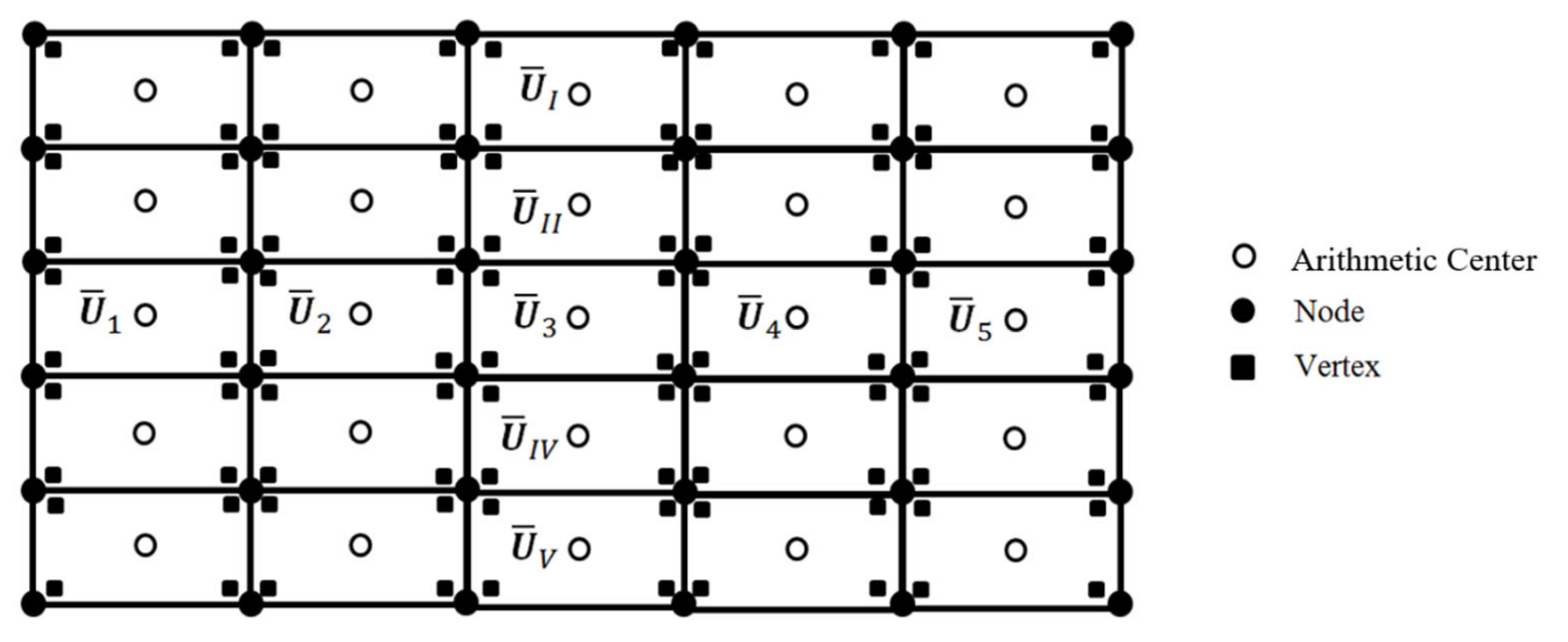
Slope limiters are required in discontinuous Galerkin methods to remove high-frequency spurious oscillations around shock waves, and to maintain high order accuracy in smooth regions. In this study, we developed a new slope limiter for discontinuous quadrilateral elements based on the explicit dissipative interface of Rosman [18]. The Rosman dissipative interface is part of the SisBahia^® (Sistema Base de Hidrodinámica Ambiental) hydrodynamic model, which is a continuous Galerkin depth-integrated shallow water model. The SisBahia^® interface smooths the nodal oscillations by modifying the computed nodal values of the variables using computed nodal values from adjacent nodes while preserving the amplitude of the phenomenon of interest. Here, the SisBahia^® interface is used to smooth the averaged nodal value in the center of the element and subsequently use this smoothed averaged value to reconstruct the values at the four nodes of the element.

The application of the new slope limiter begins by computing the element average solution of the conserved variable, ${\overline{U}}_e$, for all elements e, as given by Equation (27); where $U_{e,j}$ are the nodal values of the conserved variable on element e.

$${\overline{U}}_e=\frac{1}{4}{\displaystyle \sum }_{j=1}^4{U}_{e,j}, U_{e,j}\in \mathit{U}$$

(27)

Although the slope limiter can be applied to general linear quadrilateral elements, a discretization using linear rectangular elements is shown in Figure 1. The element average solution ${\overline{U}}_e$ is situated at the arithmetic average of the vertices (arithmetic center), as seen in Figure 1. The squares in the figure are the element nodal values located at the vertex of a rectangular element. The smoothing of ${\overline{U}}_e$ is achieved by the application of a dissipative interface. A usual dissipative interface, like the one presented by Abbot & Basco [23] in a finite difference context, applied to the center value ${\overline{U}}_3$ in Figure 1, would be:

$${\overline{U}}_3^l=\left(1-\omega \right){\overline{U}}_3+\omega \left(\frac{{\Delta }_{23}{\overline{U}}_4+{\Delta }_{34}{\overline{U}}_2}{{\Delta }_{23}+{\Delta }_{34}}\right)$$

(28)

where $\omega =\left[0,1\right]$ is a ponderation weight, and ${\Delta }_{23}$, ${\Delta }_{34}$ are the distances from ${\overline{U}}_2$ to ${\overline{U}}_3$, and from ${\overline{U}}_3$ to ${\overline{U}}_4$, respectively. An anti-dissipative interface was created by Rosman [18] to maintain the local declivity of the variables:

$${\overline{U}}_3^l=\left(1-\frac{\omega }{2}\right){\overline{U}}_3+\omega \left(\frac{{\Delta }_{23}{\overline{U}}_4+{\Delta }_{34}{\overline{U}}_2}{{\Delta }_{23}+{\Delta }_{34}}\right)-\frac{\omega }{2}\left(\frac{{\Delta }_{13}{\overline{U}}_5+{\Delta }_{35}{\overline{U}}_1}{{\Delta }_{13}+{\Delta }_{35}}\right)$$

(29)

The final form of the dissipative interface proposed by Rosman [18] is the average between (28) and (29):

$${\overline{U}}_3^{l*}=\left(1-\frac{3}{4}\omega \right){\overline{U}}_3+\omega \left(\frac{{\Delta }_{23}{\overline{U}}_4+{\Delta }_{34}{\overline{U}}_2}{{\Delta }_{23}+{\Delta }_{34}}\right)-\frac{\omega }{4}\left(\frac{{\Delta }_{13}{\overline{U}}_5+{\Delta }_{35}{\overline{U}}_1}{{\Delta }_{13}+{\Delta }_{35}}\right)$$

(30)

The value of ω = 0.5 is commonly used in the applications. To maintain symmetry, in our study we further apply the interface also in the orthogonal direction:

$${\overline{U}}_3^l=\left(1-\frac{3}{4}\omega \right){\overline{U}}_3^{l*}+\omega \left(\frac{{\Delta }_{II3}{\overline{U}}_{IV}+{\Delta }_{3IV}{\overline{U}}_{II}}{{\Delta }_{II3}+{\Delta }_{3IV}}\right)-\frac{\omega }{4}\left(\frac{{\Delta }_{I3}{\overline{U}}_V+{\Delta }_{3V}{\overline{U}}_I}{{\Delta }_{I3}+{\Delta }_{3V}}\right)$$

(31)

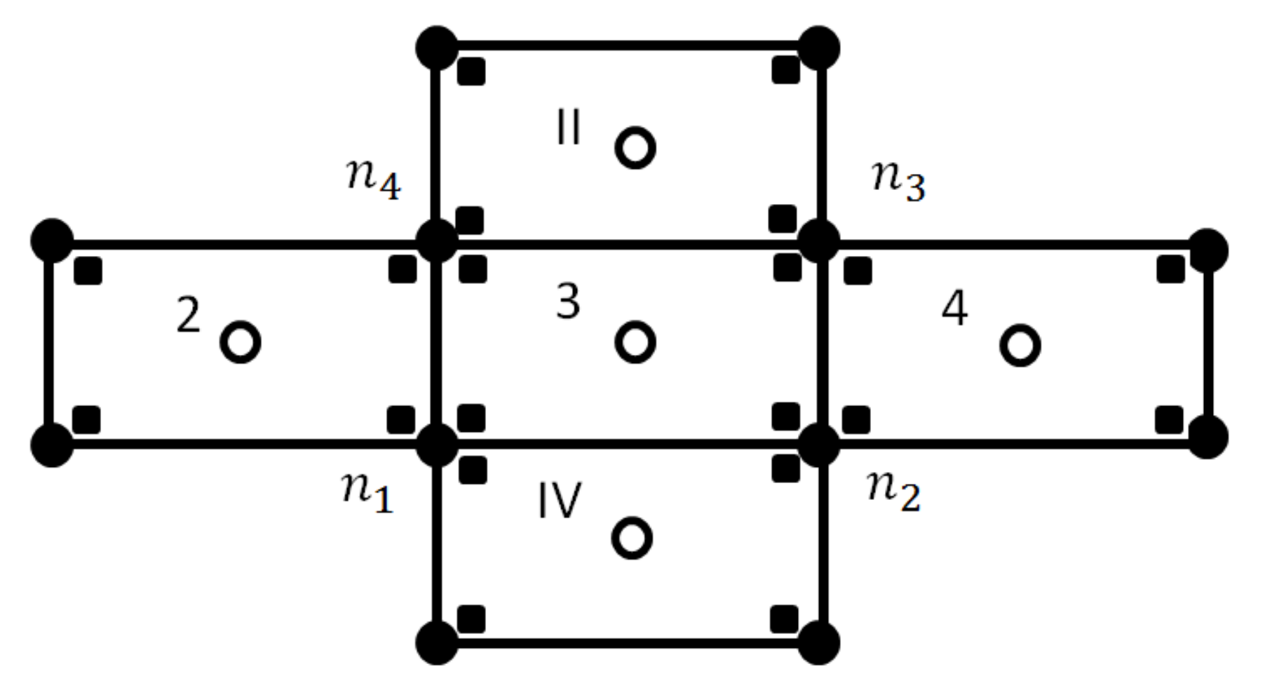
Following the limiter application procedure, the limited gradients for all elements are calculated next using Green’s theorem. An example of the evaluation of the limited gradient for the element 3 in Figure 2 is given by Equation (32).

$$\{\begin{array}{c}{\left.\frac{\partial U^l}{\partial x}\right|}_3=\frac{1}{{\Omega }_3}\underset{{\Gamma }_0}{\overset{}{\oint }}{U}^{l}dy=\frac{1}{{\Omega }_3}{\displaystyle {\displaystyle \sum }_{e=1}^4}{U}_{3e}^l{\Delta y}_e\\ {\left.\frac{\partial U^l}{\partial x}\right|}_3=\frac{1}{{\Omega }_3}\left\{U_{3\mathrm{IV}}^l\left(y_{n2}-y_{n1}\right)+U_{34}^l\left(y_{n3}-y_{n2}\right)+U_{3\mathrm{II}}^l\left(y_{n4}-y_{n3}\right)+U_{32}^l\left(y_{n1}-y_{n4}\right)\right\}\\ {\left.\frac{\partial U^l}{\partial y}\right|}_3=\frac{-1}{{\Omega }_3}\underset{{\Gamma }_0}{\overset{}{\oint }}{U}^{l}dx=\frac{-1}{{\Omega }_3}{\displaystyle {\displaystyle \sum }_{e=1}^4}{U}_{3e}^l{\Delta x}_e\\ {\left.\frac{\partial U^l}{\partial y}\right|}_3=\frac{1}{-{\Omega }_3}\left\{U_{3\mathrm{IV}}^l\left(x_{n2}-x_{n1}\right)+U_{34}^l\left(x_{n3}-x_{n2}\right)+U_{3\mathrm{II}}^l\left(x_{n4}-x_{n3}\right)+U_{32}^l\left(x_{n1}-x_{n4}\right)\right\}\end{array}$$

(32)

In Equation (32), $U_{3IV}^l$ is the limited value at the boundary between elements 3 and IV. The inverse distance weighting with ${\overline{U}}_3^l$ and ${\overline{U}}_{IV}^l$ is used to find $U_{3IV}^l$ at the boundary. A similar process is adopted to calculate $U_{34}^l$, $U_{3II}^l$ and $U_{32}^l$. Finally, the nodal values of the limited conservative variables $U_e^l$ can be reconstructed over a quadrilateral element e by evaluating Equation (33) at the four nodes. In Equation (33) $\mathit{r}$ is a vector with origin at the arithmetic center of the element extending to any point within the element. The vector $\mathit{r}$ for the node 1 at Figure 2 will be $x_{n1}-\overline{x}$, $y_{n1}-\overline{y}$, where $\overline{x} and \overline{y}$ are the values at the arithmetic center of the element. This reconstruction implies that the reconstructed variables will have a constant gradient over the element. The limiter is applied after every step of the Runge–Kutta integration in Equation (25).

$$U_3^l\left(x,y\right)={\overline{U}}_3^l+\nabla U_3^l·r$$

(33)

2.2.3. Second Step: Continuous Galerkin Solution

In the second step of the solution, a Poisson equation is constructed that is then solved by a continuous Galerkin method to obtain the non-hydrostatic pressures $q_b^{n+1}$. A time approximation of the vertical moment Equation in (4) is:

$$w_{\xi }^{n+1}=w_{\xi }^n-w_b^{n+1}+w_b^n+\frac{2\Delta t{q}_b^{n+1}}{\rho H^n}$$

(34)

The vertical velocity at the bottom is valued from the kinematic boundary condition (6), estimated as:

$$w_b^{n+1}=-U^n\frac{\partial h}{\partial x}-V^n\frac{\partial h}{\partial y}$$

$$w_b^n=-U^{n-1}\frac{\partial h}{\partial x}-V^{n-1}\frac{\partial h}{\partial y}$$

(35)

From the remaining part of the horizontal momentum Equations (1) and (2) including the non-hydrostatic pressure terms:

$$\frac{\partial \left(HU\right)}{\partial t}=-\frac{H}{2\rho }\frac{\partial q_b}{\partial x}-\frac{q_b}{2\rho }\frac{\partial \left(\xi -h\right)}{\partial x}$$

$$\frac{\partial \left(HV\right)}{\partial t}=-\frac{H}{2\rho }\frac{\partial q_b}{\partial y}-\frac{q_b}{2\rho }\frac{\partial \left(\xi -h\right)}{\partial y}$$

(36)

the final horizontal velocities, influenced by the non-hydrostatic pressure, can be time approximated as:

$${ U}_c^{n+1}={\tilde{U} }^{n+1}-\frac{\Delta t}{2\rho }\frac{\partial q_b^{n+1}}{\partial x}-\frac{\Delta t}{2\rho }\frac{q_b^{n+1}}{H_c^n}\frac{\partial }{\partial x}\left({\xi }_c^n-h\right)$$

$$V_c^{n+1}={\tilde{V}}^{n+1}-\frac{\Delta t}{2\rho }\frac{\partial q_b^{n+1}}{\partial y}-\frac{\Delta t}{2\rho }\frac{q_b^{n+1}}{H_c^n}\frac{\partial }{\partial y}\left({\xi }_c^n-h\right)$$

(37)

In the continuous Galerkin solution of the non-hydrostatic pressures, the continuous horizontal velocities $U_c^{n+1}$ and $V_c^{n+1}$, continuous water level ${\xi }_c^n$ and flow depth $H_c^n$, vertical velocities $w_{\xi }$ and $w_b,$ and non-hydrostatic pressures $q_b^{n+1}$ are approximated with nodal variables which have the same value in all the adjoining elements. The continuous intermediate velocities $\tilde{U}{ }^{n+1}$ and $\tilde{V}{ }^{n+1}$ are obtained from the intermediate evaluation of the discontinuous discharges ${\tilde{q}}_x^{n+1} and {\tilde{q}}_y^{n+1}$ integrating over the entire domain $\Omega$, as in Dawson et al. [16]:

$${\int }_{\Omega }^{}{\phi \tilde{U} }^{n+1}d\Omega ={\int }_{\Omega }^{}{\phi \tilde{U} }_{dc}^{n+1}d\Omega$$

$${\int }_{\Omega }^{}{\phi \tilde{V} }^{n+1}d\Omega ={\int }_{\Omega }^{}{\phi \tilde{V} }_{dc}^{n+1}d\Omega$$

(38)

where the discontinuous intermediate velocities ${\tilde{U}}_{dc}^{n+1}$ and ${\tilde{V}}_{dc}^{n+1}$ are approximated in an element using the values of $\frac{{\tilde{q}}_x^{n+1}}{H^n}$ and $\frac{{\tilde{q}}_y^{n+1}}{H^n}$, respectively, evaluated at the nodes. Similarly, the continuous water level elevations ${\xi }_c^n$ are obtained from:

$${\int }_{\Omega }^{}\phi {\xi }_c^{n}d\Omega ={\int }_{\Omega }^{}\phi {\xi }^{n}d\Omega$$

(39)

where ${\xi }^n=H^n-h$. Finally, the continuous flow depth, $H_c^n$, is $H_c^n={\xi }_c^n+h$. To obtain a correct solution between the velocity field and the non-hydrostatic pressures, the continuity equation is applied directly to the water column:

$$\left(\frac{\partial U_c^{n+1}}{\partial x}+\frac{\partial V_c^{n+1}}{\partial y}\right)+\left(\frac{w_{\xi }^{n+1}-w_b^{n+1}}{H_c^n}\right)=0$$

(40)

Substituting Equations (34), (35) and (37) in Equation (40), applying Green’s theorem in some terms, and neglecting others, a Poisson equation is established from which the hydrostatic pressure in the bottom, $q_b^{n+1}$, is obtained. A continuous Galerkin finite element model to solve the Poisson equation on an element ${\Omega }_e$ is:

$$\begin{array}{c}{\int }_{{\Omega }_e}\phi \frac{2{\Delta \mathrm{tq}}_b^{n+1}}{\rho {\left(H_c^n\right)}^2}{d\Omega }_{}+{\int }_{{\Omega }_e}\frac{\partial \phi }{\partial x}\frac{\Delta t}{2\rho }\frac{\partial q_b^{n+1}}{\partial x}{d\Omega }_{}+{\int }_{{\Omega }_e}\frac{\partial \phi }{\partial y}\frac{\Delta t}{2\rho }\frac{\partial q_b^{n+1}}{\partial y}{d\Omega }_{}\hfill \\ \hspace{1em}\hspace{1em}\hspace{1em}\hspace{1em}\hspace{1em}-{\int }_{{\Omega }_e}\phi \frac{\Delta t}{2{\rho H}_c^n}\frac{\partial q_b^{n+1}}{\partial x}\frac{\partial }{\partial x}\left({\xi }_c^n-h\right){d\Omega }_{}-{\int }_{{\Omega }_e}\phi \frac{\Delta t}{2{\rho H}_c^n}\frac{\partial q_b^{n+1}}{\partial y}\frac{\partial }{\partial y}\left({\xi }_c^n-h\right){d\Omega }_{} \\ \hspace{1em}\hspace{1em}\hspace{1em}\hspace{1em}=-{\int }_{{\Omega }_e}\phi \begin{array}{c}\left(\frac{\partial \tilde{U}{ }^{n+1}}{\partial x}+\right.\end{array} \frac{\partial \tilde{V}{ }^{n+1}}{\partial x} \left.+\frac{\left(w_{\xi }^n+w_b^n-2w_b^{n+1}\right)}{H_c^n}\right) d{\Omega }_{} \end{array}$$

(41)

After all the variables in Equation (41) have been approximated as in Equation (18), and all the elements of the domain have been assembled, the resulting linear system is solved to obtain the non-hydrostatic pressures $q_b^{n+1}.$

2.2.4. Third Step

Once the non-hydrostatic pressures $q_b^{n+1}$ are known, the Equations (36) are solved on an element to obtain the final solutions for the discharges $q_x^{n+1}$ and $q_y^{n+1}$. A Galerkin finite element model to solve the Equations (36) on an element ${\Omega }_e$ is:

$${\int }_{{\Omega }_e}^{}{\phi q}_x^{n+1}d\Omega ={\int }_{{\Omega }_e}^{}{\phi q ˜}_x^{n+1}d\Omega -{\int }_{{\Omega }_e}^{}\phi \frac{\Delta {\mathrm{tH}}^n}{2\rho }\frac{\partial q_b^{n+1 }}{\partial x}d\Omega -{\int }_{{\Omega }_e}^{}\phi \frac{\Delta {\mathrm{tq}}_b^{n+1 }}{2\rho }\frac{\partial \left({\xi }^n-h\right)}{\partial x}d\Omega$$

$${\int }_{{\Omega }_e}^{}{\phi q}_y^{n+1}d\Omega ={\int }_{{\Omega }_e}^{}{\phi q ˜}_y^{n+1}d\Omega -{\int }_{{\Omega }_e}^{}\phi \frac{\Delta {\mathrm{tH}}^n}{2\rho }\frac{\partial q_b^{n+1 }}{\partial y}d\Omega -{\int }_{{\Omega }_e}^{}\phi \frac{\Delta {\mathrm{tq}}_b^{n+1 }}{2\rho }\frac{\partial \left({\xi }^n-h\right)}{\partial y}d\Omega$$

(42)

The slope limiter is applied to the values of $q_x^{n+1}$, $q_y^{n+1}$ found from the expressions above. Finally, with the discharges $q_x^n$, $q_y^n,$ $q_x^{n+1}$, $q_y^{n+1}$ and the flow depth $H^n$ known, the unknown flow depth $H^{n+1}$ is calculated from the continuity Equation (3) using the second order Runge–Kutta solution (Equation (25)) of the discontinuous Galerkin formulation (Equation (17)).

2.2.5. Boundary Conditions

At wall boundaries, the condition imposed is that the gradients of water elevations and the velocities normal to the boundary are set to zero. At open boundaries, the water elevations are determined by a Sommerfeld radiation condition. At wave inflow boundaries, the water elevations and velocities are established with the corresponding inflow wave analytical formula, e.g., the formula of airy waves. For an incompressible flow, no boundary conditions for the non-hydrostatic pressure are required [1,4].

2.2.6. Dry Bed Treatment

To handle the dry bed condition, a small depth $H_{dry}$ = 0.001 m and zero velocity are defined at the dry nodes. If the water depth at a node is less than $H_{dry}$, then the water depth is set to $H$ = $H_{dry}$ and the velocity is set to zero. At the element boundary, if the water depth at one side is greater than $H_{dry}$ and the other side is equal to $H_{dry}$, then the numerical flux is calculated according to the dry bed location. The wave speed for dry bed located at the right or left side of the boundaries are given, respectively, by Equations (43) and (44). If the water depth on both sides of the boundary is equal to $H_{dry}$ then the numerical flux is set to zero.

$$\left\{{\begin{array}{c} S_L=u_{nL}-\sqrt{g{H}_L}\\ S_R=u_{nL}+2\sqrt{g{H}_L}\end{array}}_{} \right.$$

(43)

$$\left\{{\begin{array}{c} S_L=u_{nR}-2\sqrt{g{H}_R}\\ S_R=u_{nR}+\sqrt{g{H}_R}\end{array}}_{}\right.$$

(44)

2.2.7. Wave Breaking

Depth-averaged models are unable to reproduce both the overturning of waves, and the small-scale phenomena associated with wave breaking, therefore some kind of closure is necessary. Generally, this closure consists of two steps. The first one is a trigger mechanism to localize in space and time the start and end of breaking. The second one is a mechanism that produces a dissipation of total energy in the model.

The dissipation of energy is achieved by switching locally to the depth-integrated hydrostatic shallow water equations, representing breaking wave fronts as shocks. Based on the analogy between a hydraulic jump and a turbulent bore, energy dissipation is accounted for by ensuring conservation of mass and momentum. This approach was firstly introduced by Smit et al. [24] as the hydraulic front approximation (HFA) method for the treatment of wave breaking.

For the trigger mechanism of wave breaking, we use two different criteria. The first criterion is used for solitary waves and is the simplest to set up. Wave breaking in a node is established when $\frac{{\xi }_c^n}{h}>0.8$ [25,26,27]. This criterion is referred to as the local criterion in [28]. All the elements containing a node with the wave breaking condition $\frac{{\xi }_c^n}{h}>0.8$ are switched to the hydrostatic mode by making $q_b^{n+1 }=0, \frac{\partial q_b^{n+1 }}{\partial x}=0,$ $\frac{\partial q_b^{n+1 }}{\partial y}=0$ and $w_{\xi }$=$w_b$= $0$ in the element. The breaking closure is kept active on the wave until $\frac{{\xi }_c^n}{h}<0.4$.

The second criterion is used for regular waves and is based on the hybrid criterion, first introduced by Kazolea et al. [29]. The idea is to introduce a flagging strategy based on the occurrence of one of the following conditions:

• The surface variation criterion: a node is flagged if $\frac{\frac{\partial {\xi }_c}{\partial t}}{\sqrt{g\left|h\right|}}>ɣ$, with $ɣ$ ∈ [0.3, 0.65] depending on the type of breaker.
• The local slope angle criterion: a node is flagged if $\left|\frac{\partial {\xi }_c}{\partial x}, \frac{\partial {\xi }_c}{\partial y}\right|$ ≥ tan ϕ, with ϕ ∈ [14°, 33°] depending on the flow configuration.

The first condition is usually active in correspondence of moving waves. The second condition acts in a complementary manner and allows to detect stationary or slow-moving hydraulic jumps [30]. Flagged nodes are grouped to form a breaking region. This region is either enlarged to account for the typical roller length, as suggested in Tissier et al. [31] and Kazolea et al. [29], or deactivated, depending on the value of the Froude number at breaking, $F{r}_b=\sqrt{\frac{{\left(2 \frac{H_{max}}{H_{min}}+1\right)}^2-1}{8}}$, defined starting from the minimum and maximum wave height in the flagged zone ($H_{min}, H_{max)}$. All the elements containing a flagged node are switched in the element to hydrostatic mode by making $q_b^{n+1 }=0, \frac{\partial q_b^{n+1 }}{\partial x}=0$, $\frac{\partial q_b^{n+1 }}{\partial y}=0$ and $w_{\xi }$ = $w_b$ = $0$. The interested reader can refer to Bacigaluppi et al. [28] and references therein for more detail regarding the implementation of these detection criteria.

2.2.8. Computational Aspects

Typically, execution times for a non-hydrostatic model are about a factor of two to five times slower than their associated standard shallow water model, depending on the problem size [10]. The discontinuous Galerkin solutions are calculated using a direct method. In solving the assembled Poisson equation, and in the determination of the continuous variables from the discontinuous variables (Equations (38) and (39)), an iterative solver, the restarted GMRS with incomplete LU preconditioning is used. Equations (38) and (39) are solved usually with just one or two iterations of the restarted GMRS solver.

3. Model Verification and Validation

In this section, the model described above is verified and validated using several benchmark cases. The first case, with an analytical solution, verifies the correctness of the non-hydrostatic pressure implementation in the model. The next five sets of laboratory experiments have wave and flow features (e.g., wave propagation, breaking and runup) that are expected to be encountered in the nearshore zone, and thus are used to validate the model’s capability for nearshore wave modelling. The last case verifies the implementation of the model using general linear quadrilateral elements.

3.1. Solitary Wave Propagation Along a Constant Depth Channel

This standard case has been used to verify the dispersion characteristic of many Boussinesq-type and non-hydrostatic models. The solitary wave is a non-linear wave with finite amplitude. If the fluid is non-viscous, and the horizontal bottom is frictionless, the wave must maintain its shape and velocity throughout the propagation process.

In this study, we considered a frictionless channel 800 m long and water depth $h$ of 10 m. A Sommerfeld boundary condition based on the elevation of the water surface $\xi$ is specified at the entrance and exit of the channel. The solitary wave is initially at $x_0$= 150 m, with a wave height $A$ = 2 m. The mesh is made by square elements of sizes Δx = Δy = 1 m. Analytical solutions of free water surface elevation and velocity are given by:

$$\xi \left(x,t\right)=\frac{A}{{\cos h}^2\left(k\left(x-x_0-\mathrm{ct}\right)\right)}$$

(45)

$$U\left(x,t\right)=\frac{\xi c}{\xi +h}$$

(46)

where the celerity of the wave is $c=\sqrt{g\left(A+h\right)}$ and the wave number $k=\sqrt{\frac{3A}{4h^3}}$.

In Figure 3, the initial solitary wave and the analytical and simulated waveforms along the channel at 10, 20, 30 and 40 s are presented. It is seen that wave shape and amplitude are well preserved during simulation, verifying that the non-hydrostatic property has been well simulated by the model.

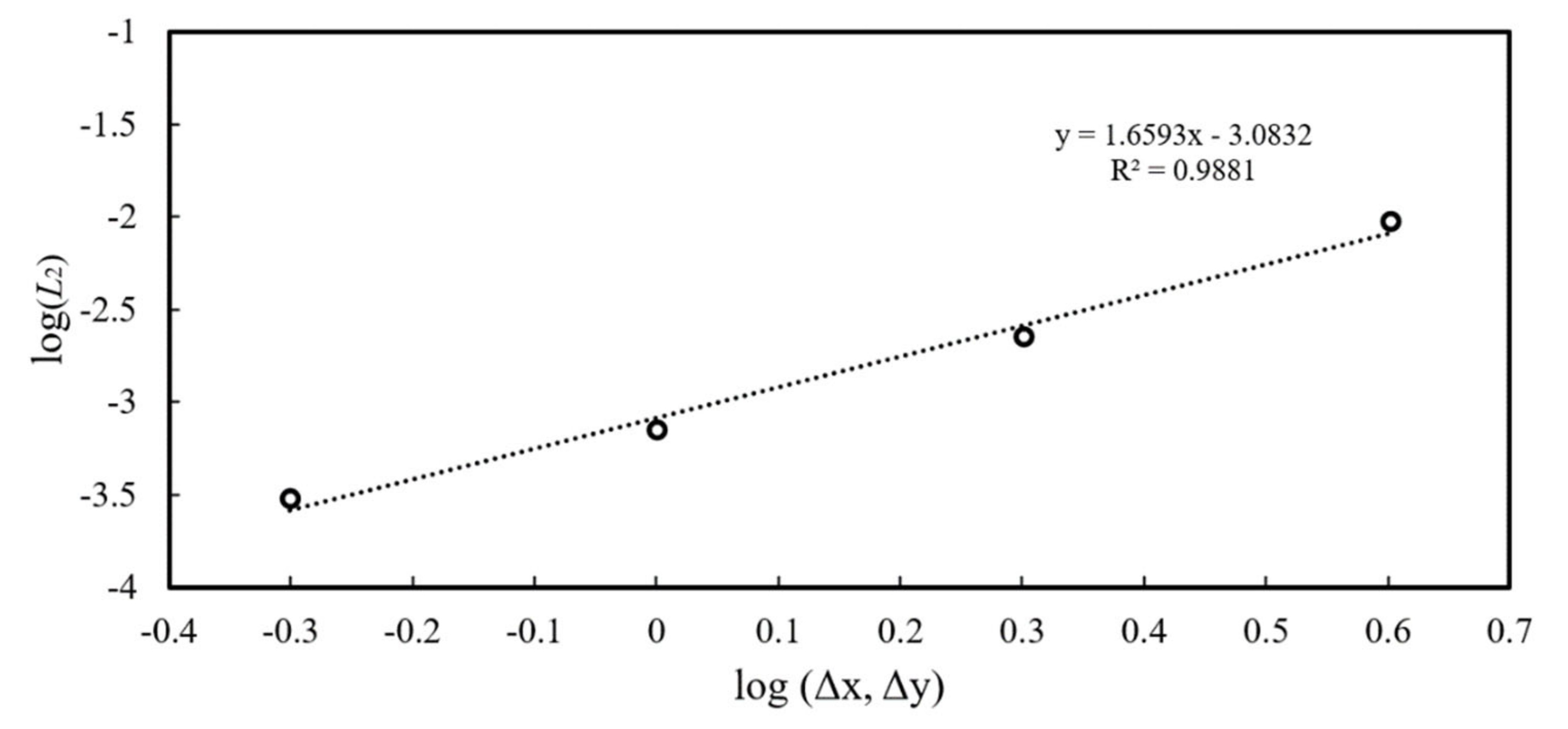
To assess the accuracy of the model, four different meshes of square elements with sizes ∆x = Δy = 0.5 m, 1.0 m, 2.0 m and 4.0 m are considered. In Figure 4, the $L_2$ error norms are shown for $\xi$ evaluated at t = 40 s as a function of grid size ∆x, Δy, defined as:

$$L_2=\frac{1}{N}\sqrt{{\displaystyle \sum }_{i=1}^N{\left({\xi }_a-{\xi }_i\right)}^2}$$

(47)

where $N$ is the total number of nodes in the direction of the flow, ${\xi }_i$ is the numerical solution and ${\xi }_a$ is the analytical solution. The numerical errors are found to be decreased when the sizes of the elements are decreased.

3.2. Solitary Wave Runup on a Plane Beach

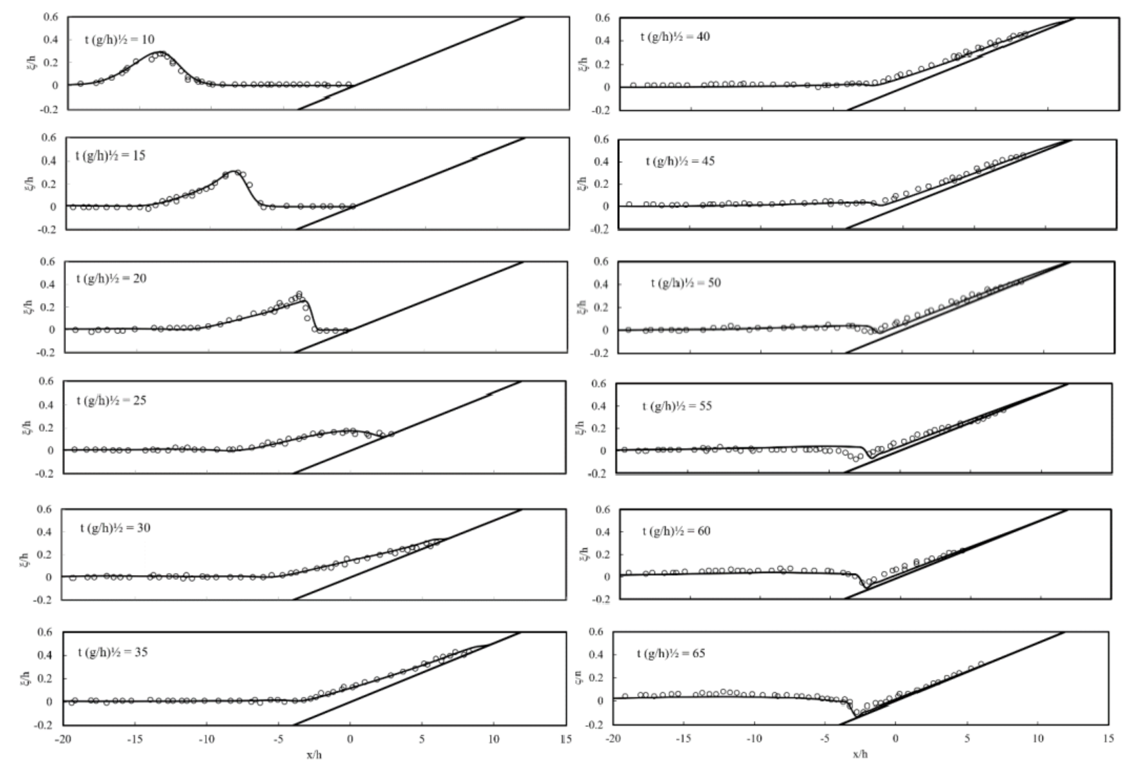
Titov & Synolakis [32] conducted experiments where a solitary wave with wave height A/h = 0.3 (where A is the solitary wave height and h is the still water depth) ran up a beach with a slope of 1:19.85. In the numerical simulation, square elements with sizes Δx/h = Δy/h = 0.125 are considered, and a Manning coefficient n = 0.01 is used to define the bed surface roughness. A Sommerfeld radiation condition is imposed at the left-side boundary. The solitary wave is initially at half of the wavelength ($L$) from the toe of the beach, with $L$ defined by:

$$L=\frac{2}{k}arccosh\left(\sqrt{\frac{1}{0.05}}\right)$$

(48)

Figure 5 shows the comparison of simulated and measured profiles. As the wave propagates over the inclined beach, the front of the wave begins to incline. Laboratory data show that the breaking of waves occurs between $t{\left(g/h\right)}^{1/2}$ = 20 and 25. The broken waves run up to the beach until the maximum height of around $t{\left(g/h\right)}^{1/2}$ = 45. It is seen that the wave breaking and runup processes are simulated very well. When the wave retreats from the beach, a hydraulic jump is formed and major discrepancy between simulated results and measured data is observed at $t{\left(g/h\right)}^{1/2}$ = 55. This phenomenon may be attributed to the complex vertical flow structure that cannot be captured by the depth-integrated formulation [30,33]. After this point, good agreements are reached until the end of the retreat process.

3.3. Solitary Wave Propagation over Fringing Reef

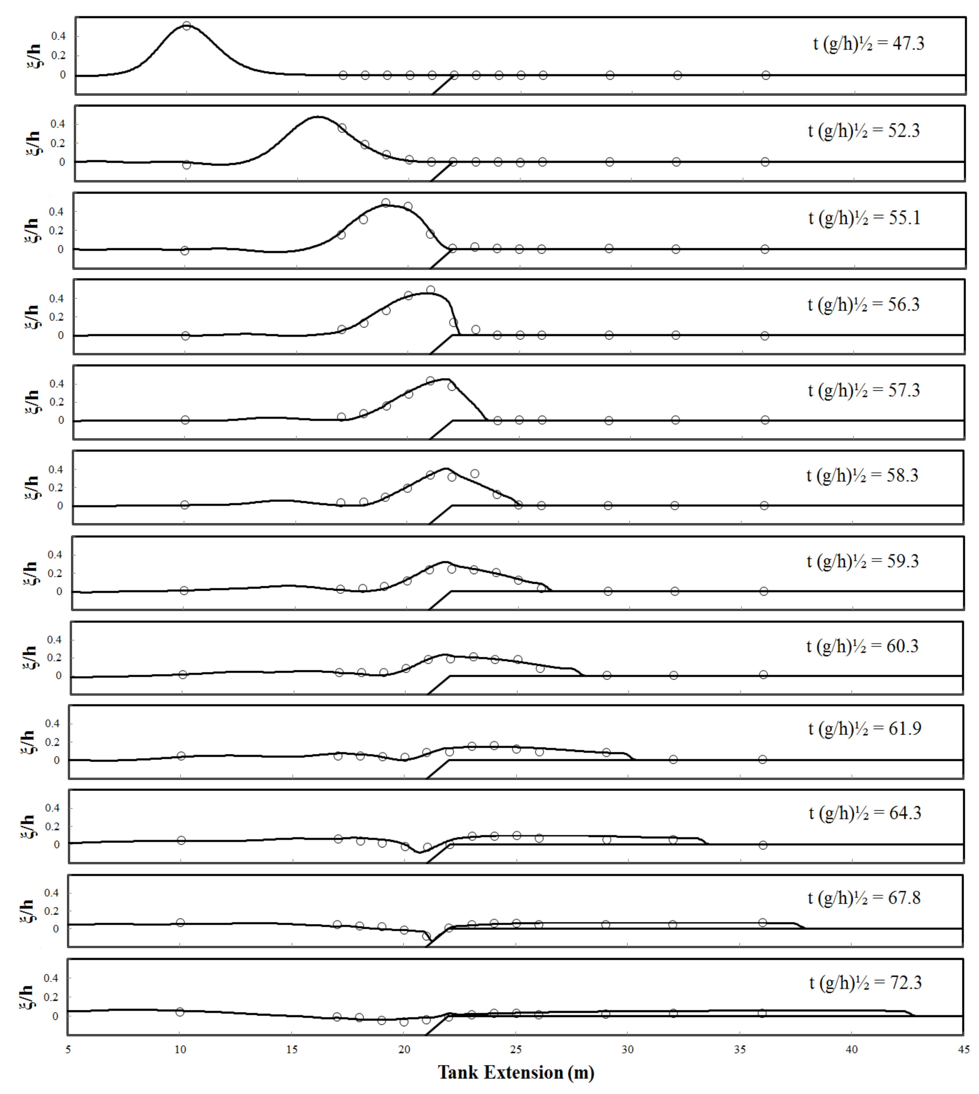
Fringing reefs are coral reefs quite common in tropical and subtropical areas. Laboratory experiments of solitary wave transformation over fringing reefs were conducted by Roeber [34] and Roeber et al. [30]. In this work, we analyze their test case consisting of a solitary wave with a height of $A$ = 0.5 m and a water depth of h = 1 m. The solitary wave is transformed over a fringing reef with a 1:5 slope onto a dry reef flat. Square finite elements with ∆x = ∆y = 0.05 m were used, and a Manning coefficient of n = 0.01 was established to represent the finished concrete surface of the reef model. A Sommerfield boundary condition is imposed at the left side of the domain.

The simulated surface elevations are compared with the measured surface elevations in Figure 6. The principal processes involved are reproduced by the model. The wave evolves from subcritical flow to supercritical flow over the reef edge at x = 22 m, collapses at x = 23 m, and subsequently rush over the initially dry reef flat. The reef edge is exposed due to the seaward movement of the reflected wave coming from the reef edge and the shoreward movement of the wave front over the reef around $t{\left(g/h\right)}^{1/2}$= 67.8. The computed results establish the ability of the model to simulate wave transformation over a fringing reef, wave breaking and wetting-drying over a dry surface.

3.4. Series of Regular Waves on a Plane Beach

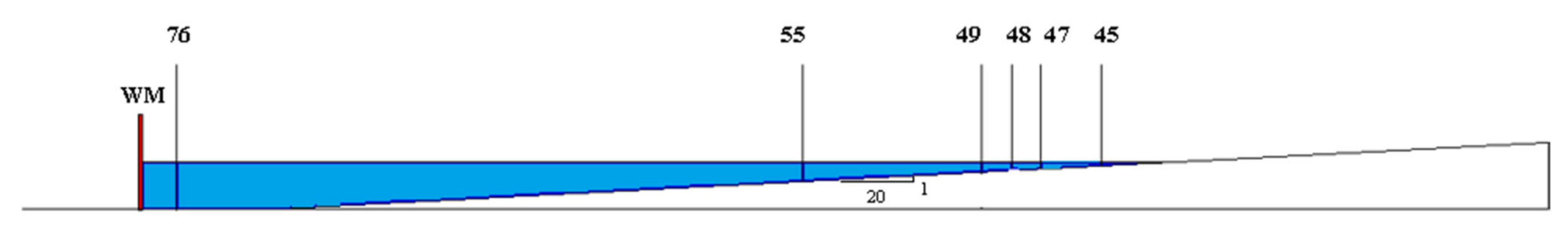
In this test, we demonstrate the ability of the model to simulate the propagation, breaking and runup of a series of regular waves. The experimental investigations were carried out at the laboratory of the Department of Civil, Environmental, Land, Building Engineering and Chemistry of the Polytechnic University of Bari, Italy. The used wave channel is 45 m long and 1 m wide, with glass walls supported by iron frames, numbered from the shoreline up to the wavemaker. Starting from the wave paddle, the flume has a flat bottom extending for 12 m, while the remaining bottom onshore is made by a wooden panel with 1/20 slope. The wave generating system is a piston-type one, with paddles producing the desired wave by providing a translation of the water mass, according to the proper input signal. Further details about the experimental tests can be found in [35,36,37].

Table 1. Experimental parameters of the analyzed regular waves.

	${\mathit{H}}_0 \left(\mathbf{cm}\right)$	T (sec)	${\mathit{L}}_0 \left(\mathbf{m}\right)$	h (m)	${\mathit{\xi }}_0$	Breaking Type
T1	11	2	4.62	0.70	0.37	Spilling
T2	6.5	4	10.12	0.70	0.74	Plunging

shows the main parameters of the examined waves listed for each experiment, such as the offshore wave height, $H_0$, the wave period T and the deepwater wavelength, $L_0$, estimated in section 76 (Figure 7), where the bottom is flat and the mean water depth, h, is equal to 0.70 m. Moreover, to evaluate the type of breaking, the Irribarren number, ${\xi }_0$, was computed for the two tests, as:

$${\xi }_0=\frac{\tan \beta }{\sqrt{\frac{H_0}{L_0}}}$$

(49)

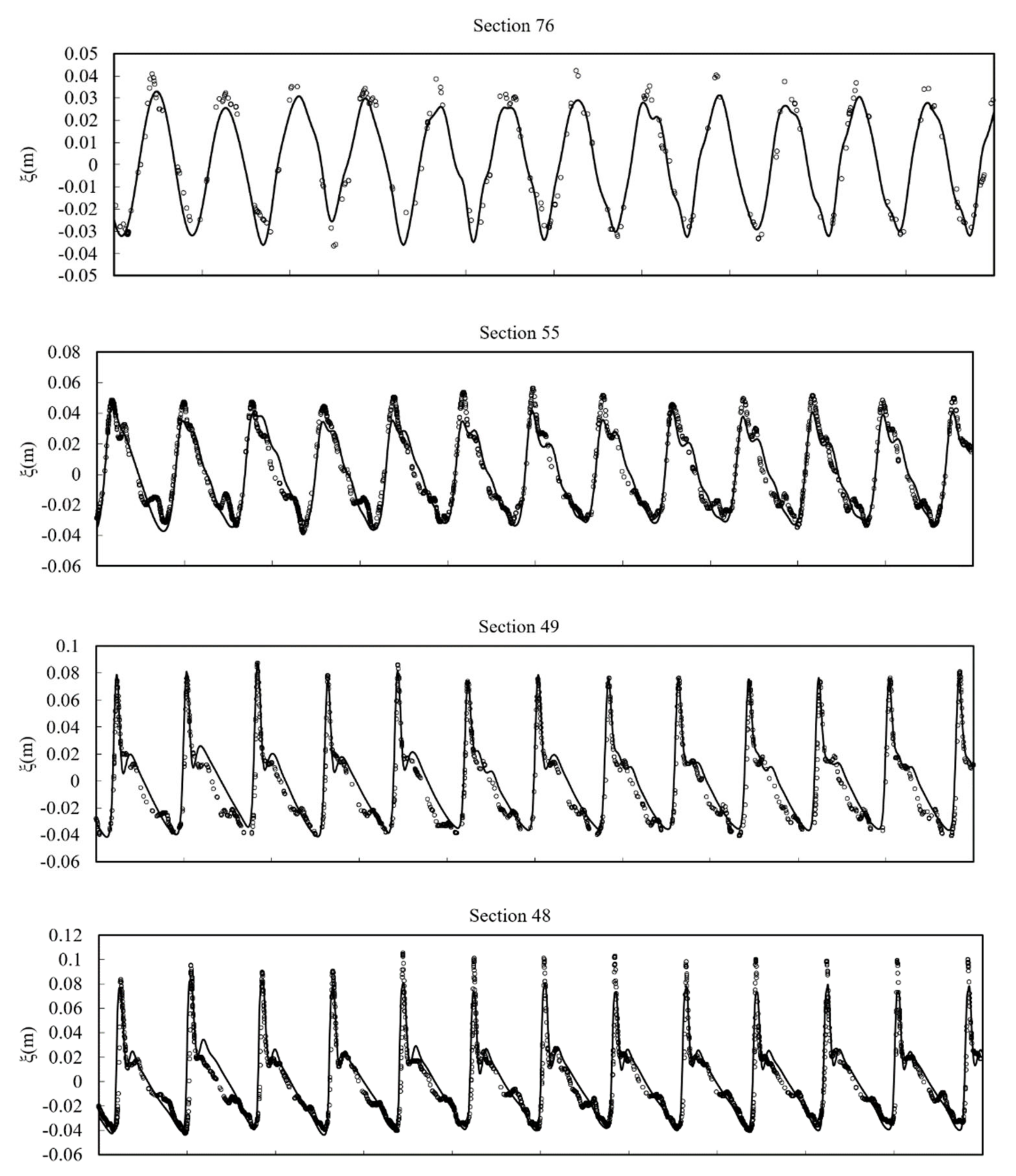
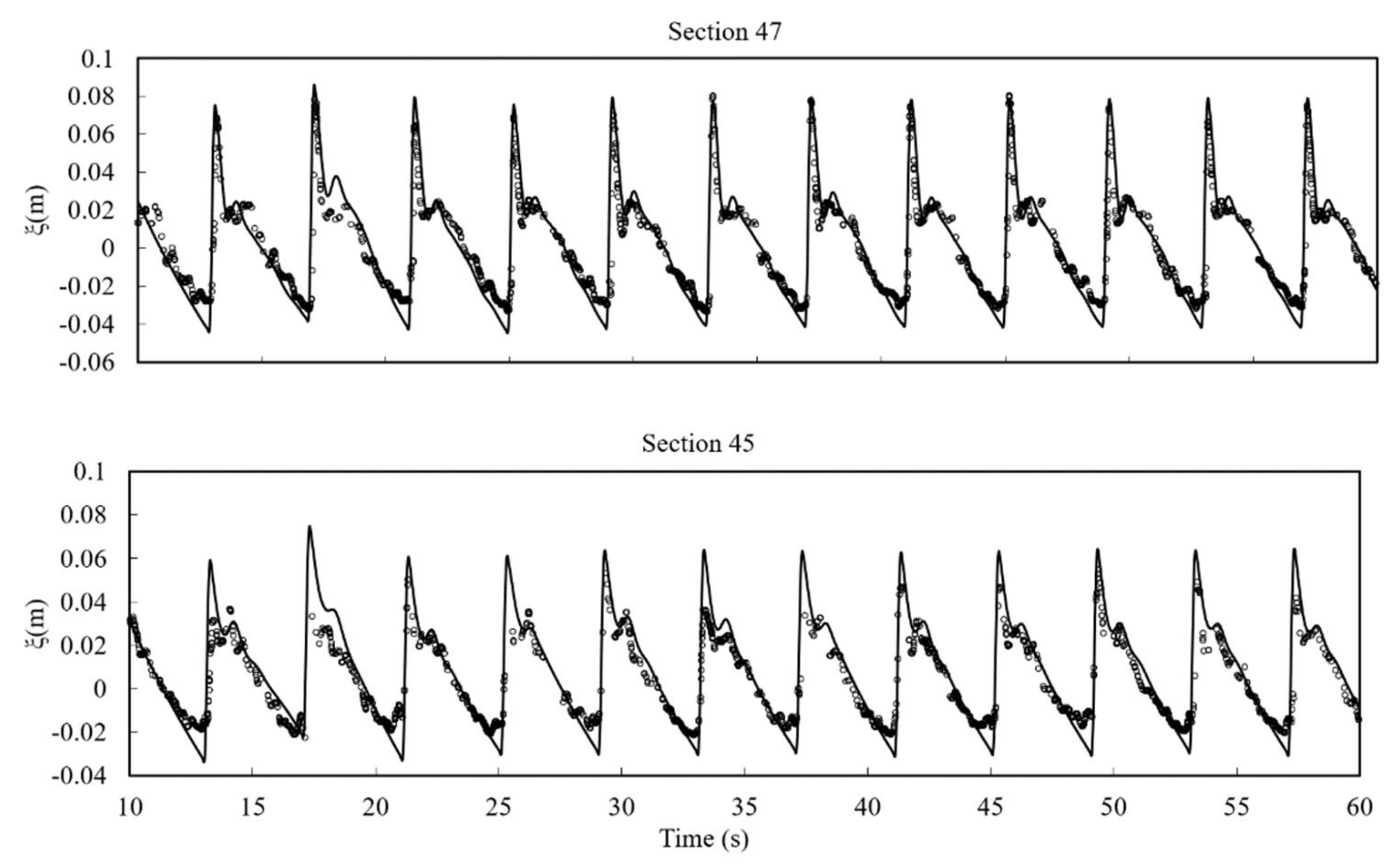
in which $\beta$ is the bottom slope angle. Based on this parameter, the two regular tested waves were characterized by a spilling and plunging breaking respectively [35]. Water surface elevations and velocities were measured at six different locations along the longitudinal axis of symmetry of the wave channel. The sketch of Figure 7 shows the six sections named 76, 55, 49, 48, 47, and 45, used in the present work for comparisons between the simulated and measured free surface elevations. Both in cases T1 and T2, the breaking occurred between sections 48 and 47.

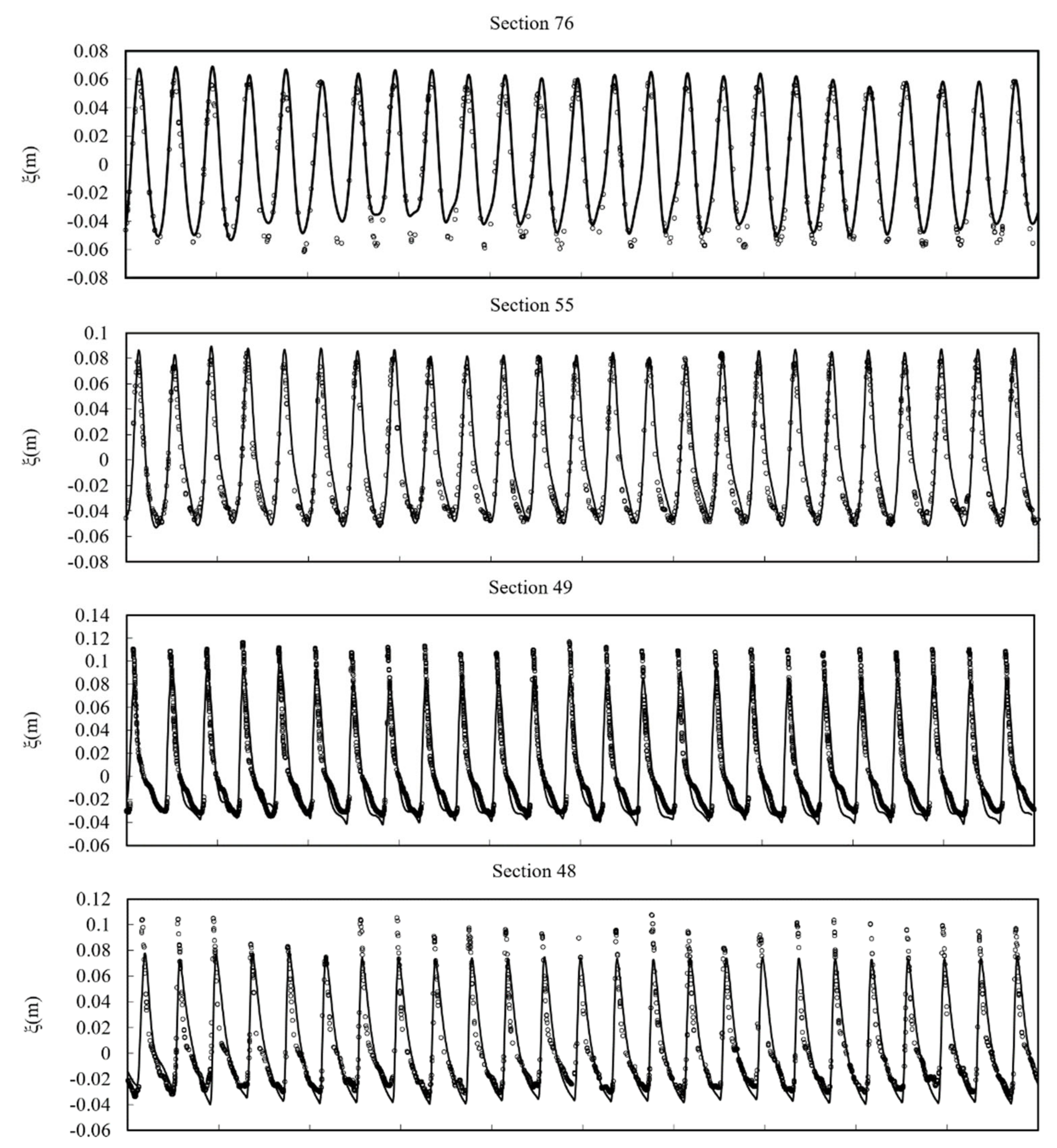
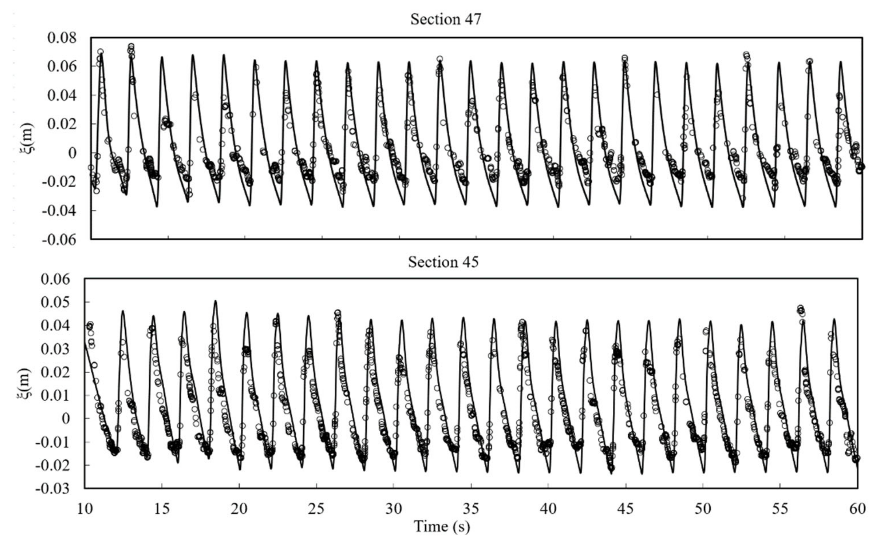
In the numerical simulation, square elements with sizes Δx = Δy = 0.04 m were considered. The time of the wave break in the numerical model is determined using the surface variation and local slope angle criteria (Section 2.2.7). Figure 8 and Figure 9 show the comparisons between the simulated and measured free surface elevations for cases T1 and T2. The surface variation criterion was utilized as the main trigger mechanism of wave breaking, and the parameter ɣ was chosen to reproduce the waves before and after the breaking zone (thus trying to match the total energy dissipation of wave breaking using the HFA method). In both case T1 (ɣ = 0.2, ϕ = 30°) and T2 (ɣ = 0.3, ϕ = 30°), similarities were obtained between the elevations of the simulated and measured waves before and after the breaking zone, except in section 48, and in section 49 for case T1 (spilling wave), where the simulated wave appears diminished. The reason for the underestimation of the breaking waves lies in the fact that the HFA method requires high vertical resolution for capturing the hydrostatic shock of the series of regular breaking waves; high vertical resolution that is obviously not present in depth-averaged models. Smit et al. [24] shows that a 3D version of a non-hydrostatic shallow water model would need as much as 20 layers to get accurate solution of wave heigh using the HFA treatment. A similar underestimation is observed in other studies using the HFA method in depth averaged models for the simulation of breaking waves series [5,28,31,38]. Attempts to improve the energy dissipation characteristics of breaking waves in depth-averaged models often involve the use of special terms in the momentum equation to account for turbulent momentum dispersion [39], or in the use of additional equations for modeling turbulent kinetic energy [38].

3.5. Solitary Wave Runup on a Conical Island

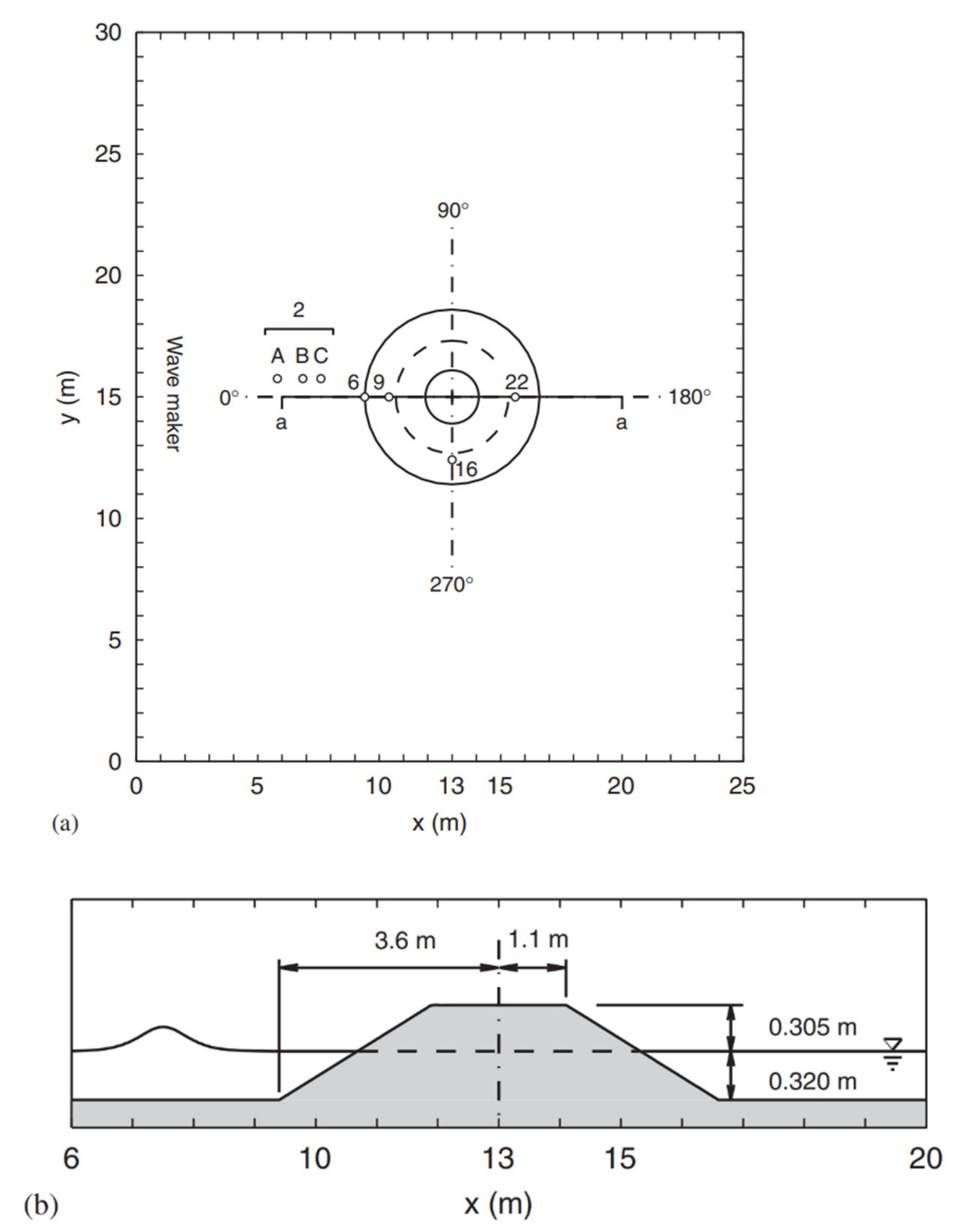
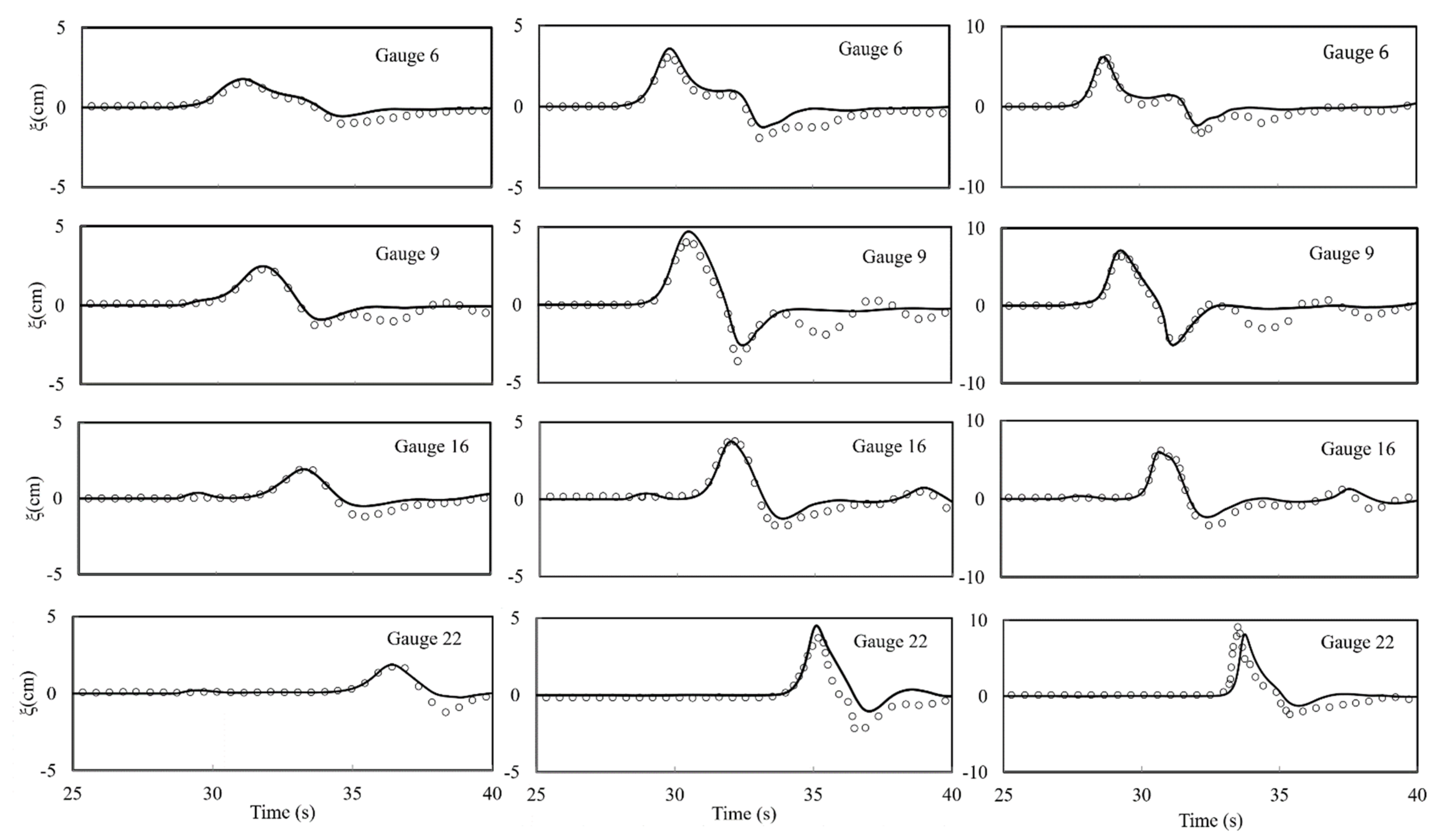
A large-scale laboratory experiment to study solitary wave runup on a conical island was conducted by Briggs et al. [40]. The experiment was conducted in a 30 m wide and 25 m long basin (Figure 10). The center of the island is located at x = 13 m and y = 15 m, and the shape of the island is a truncated circular cone with diameters of 7.2 m at the toe and 2.2 m at the crest. The vertical height of the island is about 62.5 cm, with a 1:4 beach face. A 27.4 m long directional spectral wave maker, which consisted of 61 paddles, generated solitary waves for the experiment. Wave absorbers at the three sidewalls reduced reflection. Different still water depths and relative wave heights were tested in the experiment. In this study we consider the still water depth h = 32 cm and three cases denoted as I, II, and III with relative wave heights A/h = 0.045, 0.096, and 0.181, respectively.

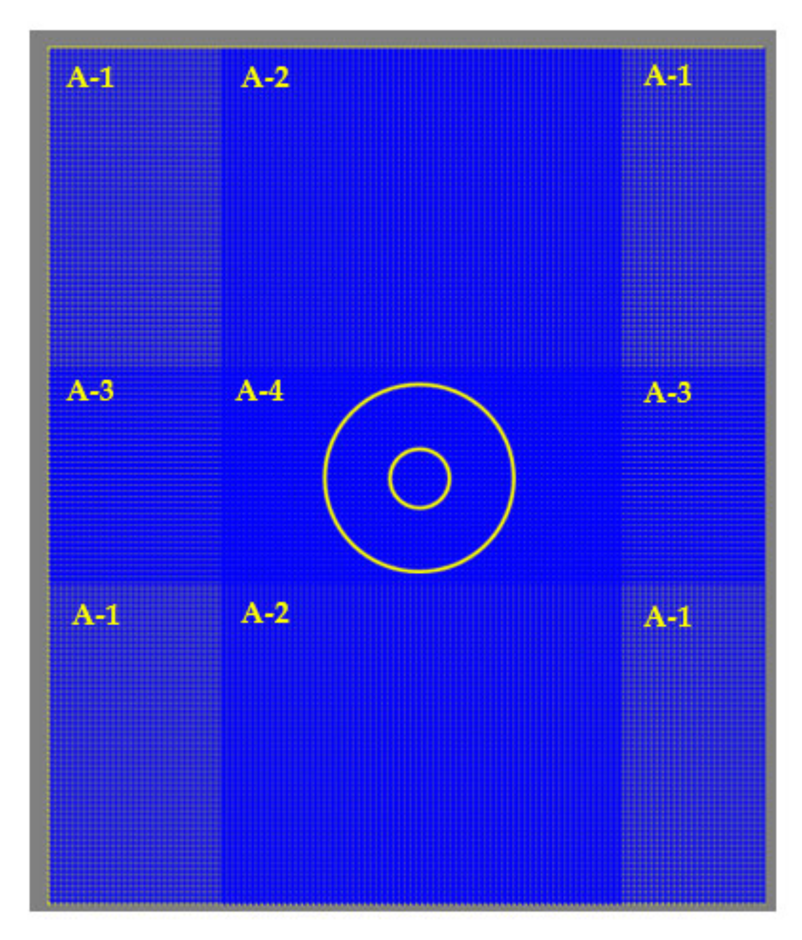
In the numerical simulation, the solitary wave propagates from the western boundary toward the island. Sommerfield radiation boundary conditions are applied at the western and eastern boundaries and the lateral walls are treated as solid walls. The basin is discretized using a total of 146,640 elements: square elements with sizes Δx = Δy = 0.1 m (A-1), rectangular elements with sizes Δx = 0.05 m and Δy = 0.1 (A-2), rectangular elements with sizes Δx = 0.1 m and Δy = 0.05 (A-3), and square elements with sizes Δx = 0.05 m and Δy = 0.05 m (A-4) near the conical island, as shown in Figure 11. The combination of rectangular and square elements reduced the number of elements/cells by 50% compared to the application of other models to the same problem, e.g., Wu et al. [8]. A Manning coefficient n = 0.01 is used for the bed surface roughness.

Figure 12 shows the comparison of simulated and measured free surface elevations at selected wave gauges for all three cases. For all cases, good agreements between numerical results and measurements are obtained in gauges 6, 9 and 16, whereas in gauge 22 overall agreements are acceptable, although the numerical model slightly overpredicts the wave depression in cases I and II.

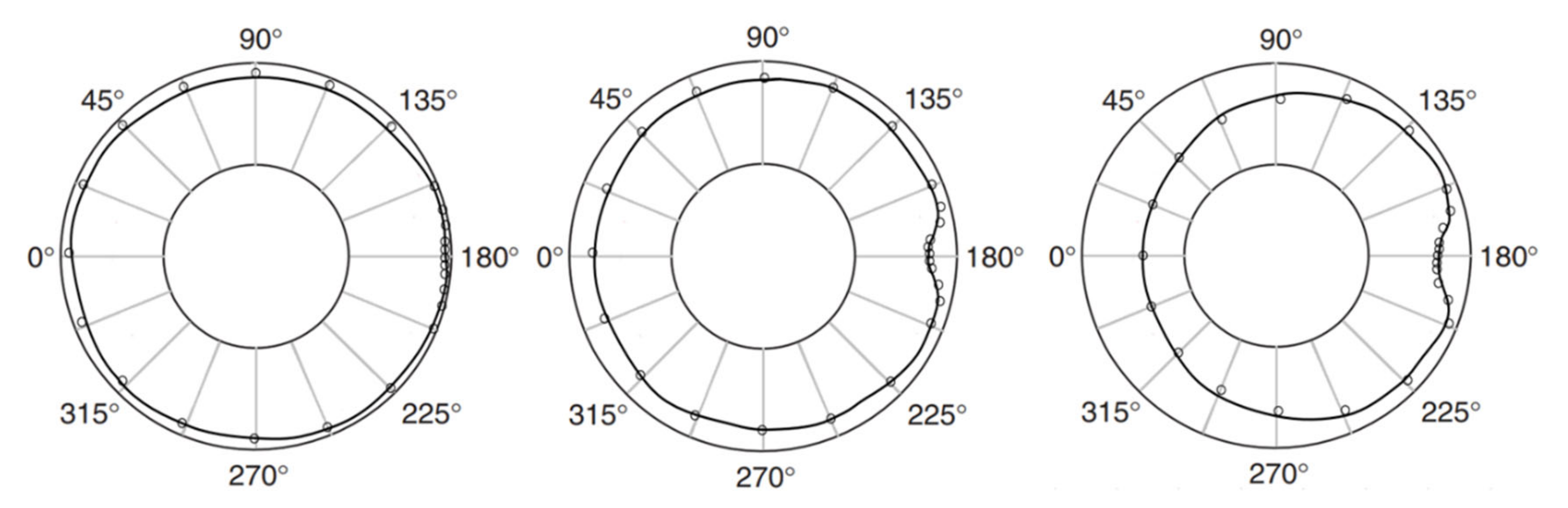
The maximum vertical runup heights are shown in Figure 13. Good agreements of the maximum inundation positions for all cases have been obtained.

3.6. Solitary Wave Transformation, Breaking and Runup over a Three-Dimensional Complex Bathymetry.

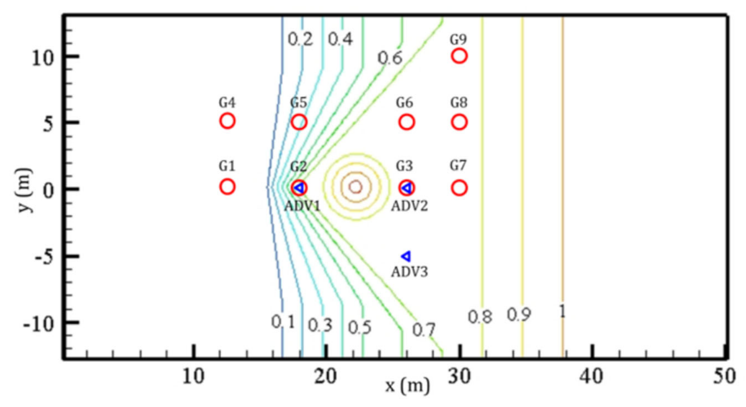
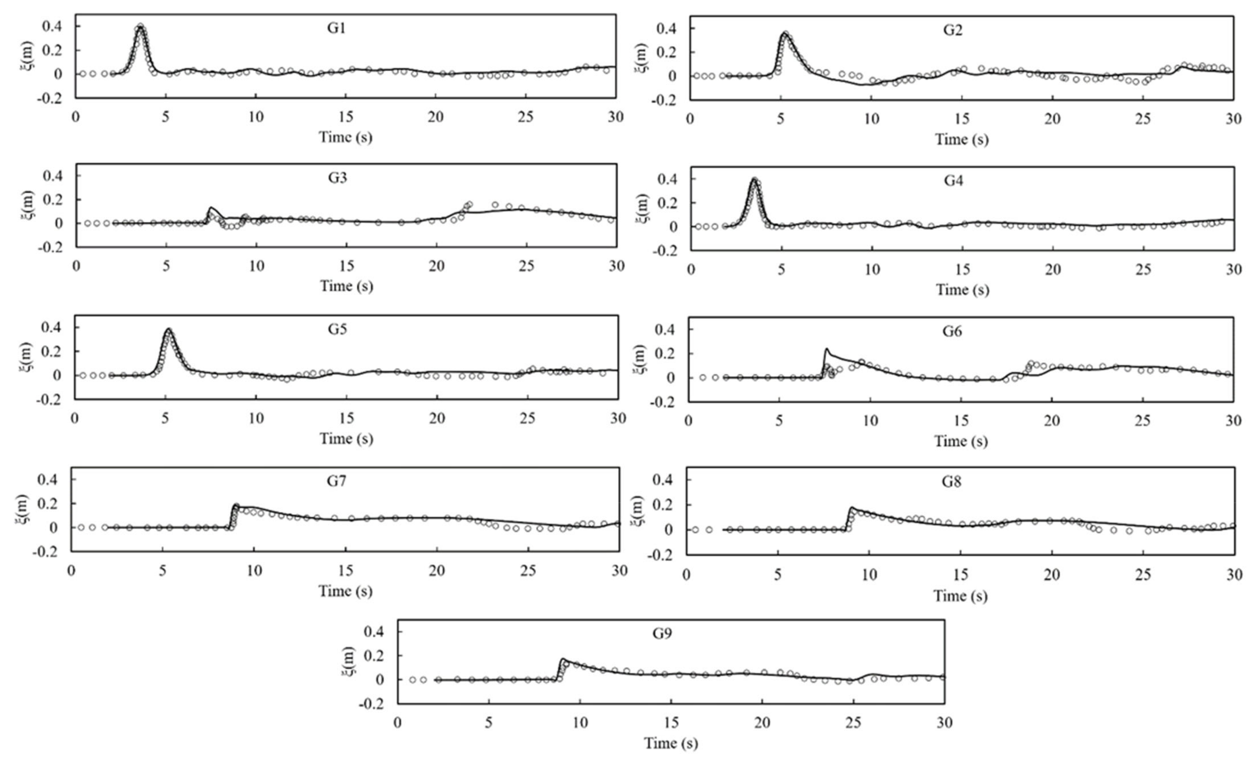
This case aims to test the model’s capacity to simulate a solitary wave transformation, breaking and runup over a 3D complex bathymetry using general quadrilateral elements. Compared to previous tests, this test is much more demanding because the wave transformation, breaking and wet-drying mechanism are implicated over a complex 3D bathymetry. Laboratory experiments were carried in a 48.8 m long and 26.5 m wide basin [41]. Figure 14 shows the basin sketch consisting of a 1:30 slope and a triangular reef flat with a conical island positioned at the offshore corner of the reef. The vertical datum for the bathymetry contours is located 0.02 m below the basin bottom. Nine wave gauges (G1-G9) were utilized to measure free surface elevation and three acoustic Doppler Velocimeters (ADV1-ADV3) were used to measure velocity, as shown in Figure 14.

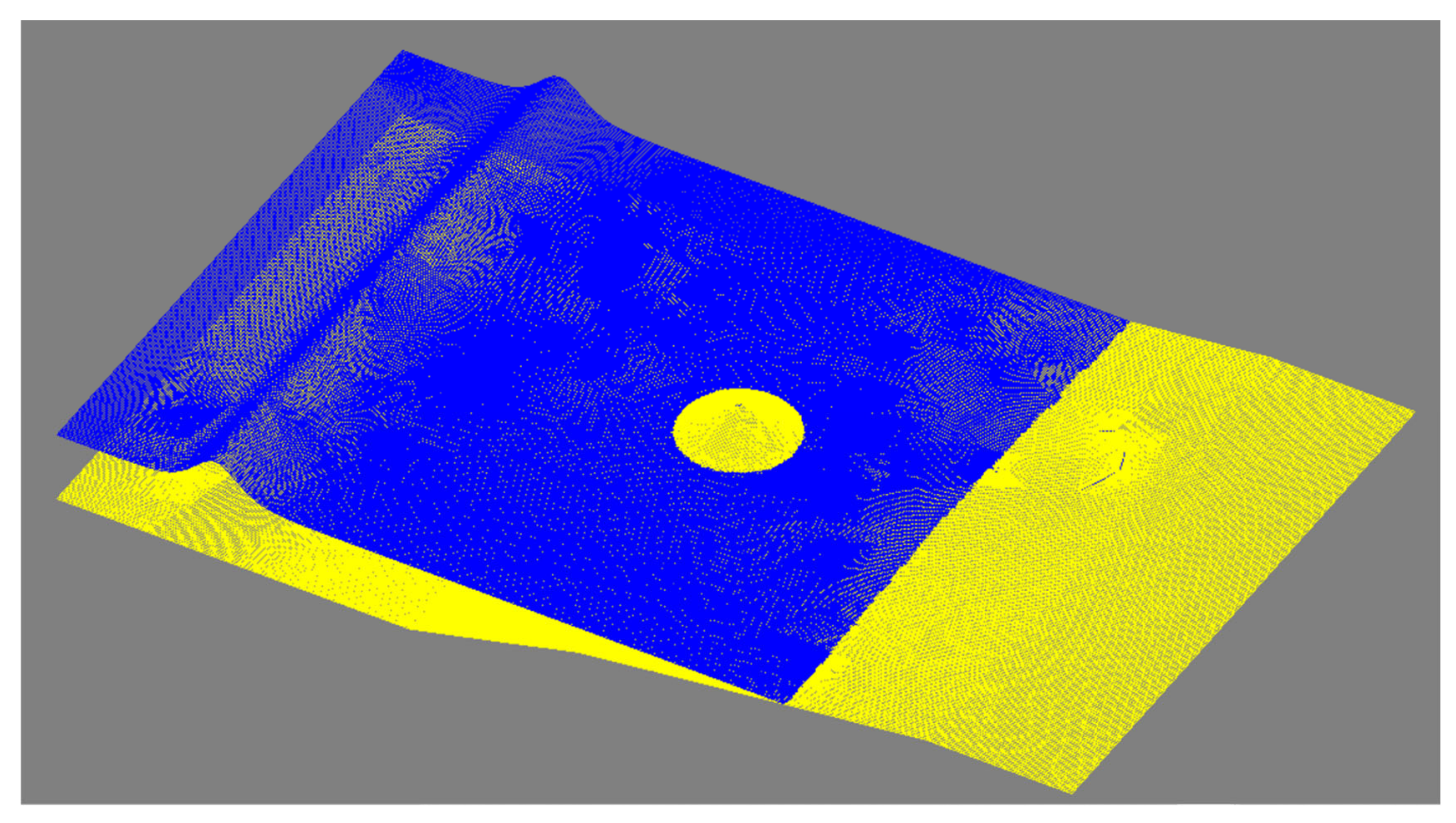
The finite element mesh consisted of 142,753 quadrilateral elements with elements areas ranging from approximately 0.01 m² to 0.0025 m² and the mesh was refined over the 3D reef around x = 16 m to x = 32 m in Figure 14. A Sommerfield radiation boundary condition is applied at the western boundary. The Manning coefficient was set to n = 0.01. The incident solitary wave has a wave height A = 0.39 m, and the water depth in the basin is h = 0.78 m. The dimensionless wave height A/h = 0.39/0.78 = 0.5 indicates a strongly nonlinear wave. The initial setup of the simulation is displayed in Figure 15.

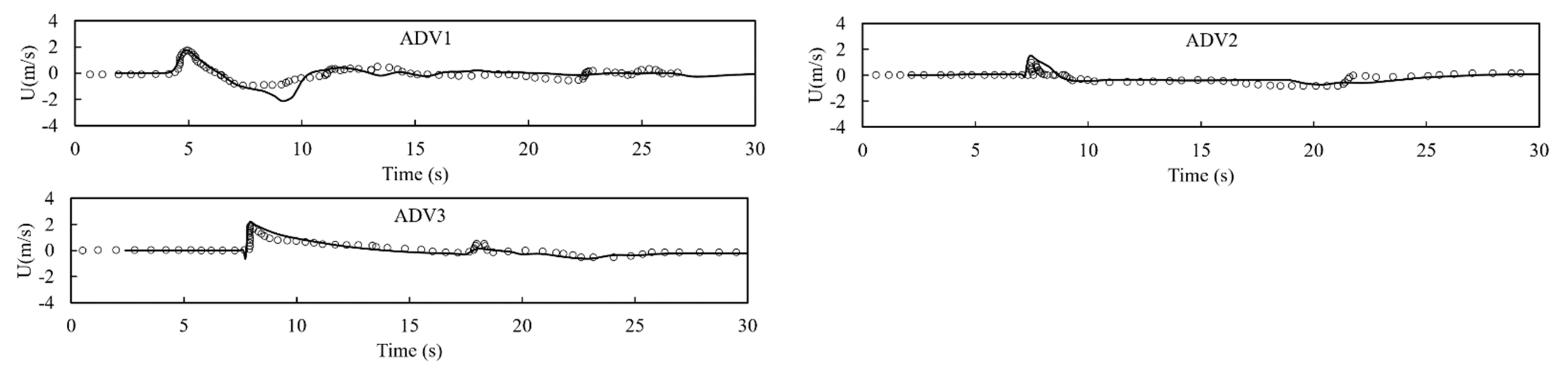
The time series of the simulated and measured free surface elevations at the nine gauge locations are presented in Figure 16. For gauges G1 and G4, located in the offshore zone, the model results and measured data agree very well, pointing that the shoreward propagation and reflection from the shore are simulated effectively. The steepening of the solitary wave over the reef tip is captured by the model at gauge G2. For gauges G3 and G6, deviations between the simulated and measured free surface elevations are registered, this was also noted in other studies [12,42]. For gauges G7, G8 and G9, the simulations are satisfactorily close to the measurements. The comparison between the computed and measured velocities in the x direction at the acoustic Doppler velocimeters locations (ADV1-ADV3) are presented in Figure 17, showing that the model is able to simulate most of the velocities’ characteristics at ADV1-ADV3. In general, the developed model succeeded in simulating a solitary wave transformation, breaking and runup over a 3D complex bathymetry. The model code, which runs on a single CPU core, was compiled using Visual Studio 2010 and the C++ language. For this test, which is the most challenging test, the CPU time was about 6.05 h on a desktop computer with an Intel^® i7-9750H CPU, at 2.6 GHz and 8 GB of memory. This performance could be improved in future developments if a CUDA^®-GPU version of the model is achieved.

4. Conclusions

A new depth-integrated non-hydrostatic, combined discontinuous/continuous, Galerkin finite element model for wave propagation, transformation, breaking and runup has been described in this paper. The formulation decomposes the depth-integrated non-hydrostatic equations into hydrostatic and non-hydrostatic parts. The hydrostatic part is equivalent to the depth-integrated shallow-water equations and was solved with a discontinuous Galerkin finite element method to allow the simulation of discontinuous flows, wave breaking and runup. The non-hydrostatic part led to a Poisson type equation, where the non-hydrostatic pressure was solved using a continuous Galerkin method to allow for the modeling of wave propagation and transformation.

The model uses linear quadrilateral finite elements for horizontal velocities, water surface elevations and non-hydrostatic pressures approximations. A new slope limiter for quadrilateral elements was developed with success based on the explicit dissipative interface of Rosman [18].

A series of numerical tests have been carried out to verify and validate the developed model. The first case, which has an analytical solution, verifies the non-hydrostatic pressure implementation in the model. The following five sets of laboratory experiments, which present several nearshore waves phenomena (e.g., nonlinear dispersive wave propagation, breaking, and runup), have been used to validate the model’s capability for nearshore wave process simulation. The last case verified the implementation of the model using general linear quadrilateral elements. Good agreements between numerical results and experimental data proved that the new depth-integrated non-hydrostatic model is applicable to simulate real-life wave motions.

In the future, the model will be extended with more layers, or a quadratic approximation of the dynamic pressure, so that highly dispersive waves can be better simulated.

References

- Casulli, V.; Stelling, G.S. Numerical simulation of 3D quasi-hydrostatic, free-surface flows. J. Hydraul. Eng. 1998, 124, 678–686. [Google Scholar] [CrossRef]
- Stansby, P.K.; Zhou, J.G. Shallow-water flow solver with non-hydrostatic pressure: 2D vertical plane problems. Int. J. Numer. Methods Fluids 1998, 28, 541–563. [Google Scholar] [CrossRef]
- Stelling, G.; Zijlema, M. An accurate and efficient finite difference algorithm for non-hydrostatic free surface flow with application to wave propagation. Int. J. Numer. Methods Fluids 2003, 43, 1–23. [Google Scholar] [CrossRef]
- Zijlema, M.; Stelling, G.S. Further experiences with computing non-hydrostatic free-surface flows involving water waves. Int. J. Numer. Methods Fluids 2005, 48, 169–197. [Google Scholar] [CrossRef]
- Zijlema, M.; Stelling, G.S. Efficient computation of surf zone waves using the nonlinear shallow water equations with non-hydrostatic pressure. Coast. Eng. 2008, 55, 780–790. [Google Scholar] [CrossRef]
- Zijlema, M.; Stelling, G.S.; Smith, P. SWASH: An operational public domain code for simulating wave fiels and rapidly varied flows in coastal waters. Coast. Eng. 2011, 58, 992–1012. [Google Scholar] [CrossRef]
- Zijlema, M. Computation of free surface waves in coastal waters with SWASH on unstructured grids. Comp. Fluids 2020, 213, 104751. [Google Scholar] [CrossRef]
- Wu, G.; Lin, Y.; Dong, P.; Zhang, K. Development of two-dimensional non-hydrostatic wave model based on central-upwind scheme. J. Mar. Sci. Eng. 2020, 8, 505. [Google Scholar] [CrossRef]
- Wang, W.; Martin, T.; Kamath, A.; Bihs, H. An improved depth-averaged non-hydrostatic shallow water model with quadratic pressure approximation. Int. J. Numer. Methods Fluids 2020, 92, 803–824. [Google Scholar] [CrossRef] [Green Version]
- Walters, R.A. A semi implicit finite element model for non-hydrostatic (dispersive) surface waves. Int. J. Numer. Methods Fluids 2005, 49, 721–737. [Google Scholar] [CrossRef]
- Wei, Z.; Jia, Y. A depth-integrated non-hydrostatic finite element model for wave propagation. Int. J. Numer. Methods Fluids 2013, 73, 976–1000. [Google Scholar] [CrossRef]
- Wei, Z.; Jia, Y. Simulation of nearshore wave processes by a depth-integrated non-hydrostatic finite element model. Coast. Eng. 2014, 83, 93–107. [Google Scholar] [CrossRef]
- Calvo, L.; Rosman, P.C. Depth Integrated Non Hydrostatic Finite Element Model for Wave Propagation. Revista I+D Tecnológico 2017, 13, 56–66. [Google Scholar]
- Bradford, S. Nonhydrostatic model for surf zone simulation. J. Waterw. Port Coast. Ocean Eng. 2011, 137, 163–174. [Google Scholar] [CrossRef]
- Choi, D.Y.; Wu, C.H.; Young, C. An efficient curvilinear non-hydrostatic model for simulating surface water waves. Int. J. Numer. Methods Fluids 2011, 66, 1093–1115. [Google Scholar] [CrossRef]
- Dawson, C.; Westerink, J.J.; Feyen, J.C.; Pothina, D. Continuous, discontinuous and coupled discontinuous–continuous Galerkin finite element methods for the shallow water equations. Int. J. Numer. Methods Fluids 2006, 52, 63–88. [Google Scholar] [CrossRef]
- Jeschke, A.; Vater, S.; Behrens, J. A discontinuous Galerkin method for non-hydrostatic shallow water flows. In Proceedings of the Conference: Finite Volumes for Complex Applications VIII-Hyperbolic, Elliptic and Parabolic Problems, Lille, France, 12–16 June 2017. [Google Scholar] [CrossRef]
- Rosman, S. Referência Técnica do SisBahia. 2019. Available online: http://www.sisbahia.coppe.ufrj.br/SisBAHIA_RefTec_V10d_.pdf (accessed on 12 April 2021).
- Hoteit, H.; Ackerer, P.; Mosé, R.; Erhel, J.; Philippe, B. New Two-Dimensional Slope Limiters for Discontinuous Galerkin Methods on Arbitrary Meshes; Research Report, RR-4491; Institut National de Recherche en Informatique et en Automatique (Inria): Paris, France, 2002. [Google Scholar]
- Stelling, G.S.; Busnelli, M.M. Numerical simulation of the vertical structure of discontinuous flows. Int. J. Numer. Methods Fluids 2001, 37, 23–43. [Google Scholar] [CrossRef]
- Bai, Y.; Cheung, K.F. Dispersion and nonlinearity of multi-layer non-hydrostatic free-surface flow. J. Fluid Mech. 2013, 726, 226–260. [Google Scholar] [CrossRef]
- Harten, A.; Lax, P.D.; van Leer, B. On upstream differencing and Godunov-type schemes for hyperbolic conservations laws. SIAM Rev. 1983, 25, 35–61. [Google Scholar] [CrossRef]
- Abbot, M.B.; Basco, D.R. Computational Fluid Dynamics, an Introduction for Engineers; Longan Group, UK Limited: London, UK, 1989. [Google Scholar]
- Smit, P.; Zijlema, M.; Stelling, G. Depth-induced wave breaking in a non-hydrostatic, near-shore wave model. Coast. Eng. 2013, 76, 1–16. [Google Scholar] [CrossRef]
- Fang, K.Z.; Zou, Z.L.; Dong, P.; Liu, Z.B.; Gui, Q.Q.; Yin, J.W. An efficient shock capturing algorithm to the extended Boussinesq wave equations. Appl. Ocean Res. 2013, 43, 11–20. [Google Scholar] [CrossRef]
- Shi, F.; Kirby, J.T.; Harris, J.C.; Geinman, J.D.; Grilli, S.T. A high-order adaptative time-stepping TVD solver for Boussinesq modeling of breaking waves and coastal inundation. Ocean Model. 2012, 43, 36–51. [Google Scholar] [CrossRef]
- Tonelli, M.; Petti, M. Hybrid finite volume-Finite difference scheme for 2DH improved Boussinesq equations. Coast. Eng. 2009, 56, 609–620. [Google Scholar] [CrossRef]
- Bacigaluppi, P.; Ricchiuto, M.; Bonneton, P. Implementation and Evaluation of Breaking Detection Criteria for a Hybrid Boussinesq Model. Water Waves 2020, 2, 207–241. [Google Scholar] [CrossRef] [Green Version]
- Kazolea, M.; Delis, A.I.; Synolakis, C.E. Numerical treatment of wave breaking on unstructured finite volume approximations for extended Boussinesq-type equations. J. Comput. Phys. 2014, 271, 281–305. [Google Scholar] [CrossRef]
- Roeber, V.; Cheung, K.F.; Kobayashi, M.H. Shock-capturing Boussinesq-type model for nearshore wave processes. Coast. Eng. 2010, 57, 407–423. [Google Scholar] [CrossRef]
- Tissier, M.; Bonneton, P.; Marche, F.; Chazel, F.; Lannes, D. A new approach to handle wave breaking in fully non-linear Boussinesq models. Coast. Eng. 2012, 67, 54–66. [Google Scholar] [CrossRef]
- Titov, V.V.; Synolakis, C.E. Modeling of breaking and nonbreaking long-wave evolution and runup using VTCS-2. J. Waterw. Port Coast. Ocean Eng. 1995, 121, 308–316. [Google Scholar] [CrossRef]
- Yamazaki, Y.; Kowalik, Z.; Cheung, K.F. Depth-integrated, non-hydrostatic model for wave breaking and run-up. Int. J. Numer. Methods Fluids 2008, 61, 473–497. [Google Scholar] [CrossRef]
- Roeber, V. Boussinesq-Type Model for Nearshore Wave Process in Fringing Reef Environment. Ph.D. Thesis, University Hawaii at Manoa, Honolulu, HI, USA, 2010. [Google Scholar]
- De Serio, F.; Mossa, M. Experimental study on the hydrodynamics of regular breaking waves. Coast. Eng. 2006, 53, 99–113. [Google Scholar] [CrossRef]
- De Padova, D.; Dalrymple, R.A.; Mossa, M. Analysis of the artificial viscosity in the smoothed particle hydrodynamics modelling of regular waves. J. Hydraul. Res. 2014, 52, 836–848. [Google Scholar] [CrossRef]
- De Padova, D.; Mouldi, B.M.; De Serio, F.; Mossa, M.; Sibilla, S. Characteristics of breaking vorticity in spilling and plunging waves investigated numerically by SPH. Environ. Fluid Mech. 2019. [CrossRef]
- Kazolea, M.; Ricchiuto, M. On Wave Breaking for Boussinesq-Type Models; Research Report RR-9092; Institut National de Recherche en Informatique et en Automatique (Inria): Prais, France, 2017. [Google Scholar]
- Hieu, P.D.; Vinh, P.N. A numerical model for simulation of near-shore waves and wave induced currents using the depth-averaged non-hydrostatic shallow water equations with an improvement of wave energy dissipation. Vietnam J. Mar. Sci. Technol. 2020, 20, 155–172. [Google Scholar] [CrossRef]
- Briggs, M.J.; Synolakis, C.E.; Harkins, G.S.; Green, D.R. Laboratory Experiments of Tsunami Runup on a Circular Island. Tsunamis: 1992–1994; Springer: Berlin/Heidelberg, Germany, 1995; pp. 569–593. [Google Scholar]
- Swigler, D.T. Laboratory Study Investigating the Three-Dimensional Turbulence and Kinematic Properties Associated with a Breaking Solitary Wave. Ph.D. Thesis, Texas A & M University, Uvalde, TX, USA, 2010. [Google Scholar]
- Fang, K.; Liu, Z.; Zou, Z. Modelling coastal water waves using a depth-integrated, non-hydrostatic model with shock-capturing ability. J. Hydraul. Res. 2015, 53, 119–133. [Google Scholar] [CrossRef]
Figure 1.
Discretization using discontinuous linear rectangular elements.
Figure 2.
Discontinuous elements used in the assessment of the limited gradient for element 3.
Figure 3.
Comparison of numerical results and analytical solutions of free surface elevations at t = 0, 10, 20, 30 and 40 s. Analytical solutions (circles), numerical results (solid lines).
Figure 4.
error norms for as function of ∆x, ∆y for solitary wave propagation in constant depth.
Figure 5.
Comparison of simulated and measured surface profiles of a solitary wave runup on a 1:19.85 plane beach. Experimental data (circles), numerical results (solid lines).
Figure 6.
Comparison of simulated and measured surface profiles of a solitary wave over a fringing reef. Experimental data (circles), numerical results (solid lines).
Figure 7.
Diagram of the channel with the location of the six investigated sections (From: De Padova et al. [37]).
Figure 8.
Comparison of simulated and measured free surface elevations for case T1 (spilling wave) (ɣ = 0.2, ϕ = 30°). Experimental data (circles), numerical results (solid lines).
Figure 9.
Comparison of simulated and measured free surface elevations for case T2 (plunging wave) (ɣ = 0.3, ϕ = 30°). Experimental data (circles), numerical results (solid lines).
Figure 10.
Schematic sketch of the conical island experiment. (a) Plane view, (b) side view, ο gauge locations (from: Yamazaki et al. [33]).
Figure 11.
Discretization of the conic island domain using rectangular elements.
Figure 12.
Comparison of simulated and measured free surface elevations for a solitary wave runup on a conical island: A/h = 0.045 (left panel), A/h = 0.096 (middle panel), A/h = 0.181 (right panel). Experimental data (circles), numerical results (solid lines).
Figure 13.
Comparison of simulated and measured maximum vertical runup heights for a solitary wave runup on a conical island: A/h = 0.045 (left panel), A/h = 0.096 (middle panel), A/h = 0.181 (right panel). Experimental data (circles), numerical results (solid lines).
Figure 14.
Bathymetry contours and locations of measuring points. Circles (water surface measurement gauges), triangles (acoustic Doppler velocimeters) (from: Wu et al. [8]).
Figure 15.
Snapshot of the initial setup of the simulation of a solitary wave transformation, breaking and runup over a three-dimensional reef.
Figure 16.
Comparison of simulated and measured free surface elevations at gauge locations. Measured data (circles), numerical results (solid lines).
Figure 17.
Comparison of simulated and measured velocities in the x direction at the acoustic Doppler velocimeters locations. Experimental data (circles), numerical results (solid lines).