Group Classification for the Search and Identification of Related Patterns Using a Variety of Multivariate Techniques

Abstract

Recently, many methods and algorithms have been developed that can be quickly adapted to different situations within a population of interest, especially in the health sector. Success has been achieved by generating better models and higher-quality results to facilitate decision making, as well as to propose new diagnostic procedures and treatments adapted to each patient. These models can also improve people’s quality of life, dissuade bad health habits, reinforce good habits, and modify the pre-existing ones. In this sense, the objective of this study was to apply supervised and unsupervised classification techniques, where the clustering algorithm was the key factor for grouping. This led to the development of three optimal groups of clinical pattern based on their characteristics. The supervised classification methods used in this study were Correspondence (CA) and Decision Trees (DT), which served as visual aids to identify the possible groups. At the same time, they were used as exploratory mechanisms to confirm the results for the existing information, which enhanced the value of the final results. In conclusion, this multi-technique approach was found to be a feasible method that can be used in different situations when there are sufficient data. It was thus necessary to reduce the dimensional space, provide missing values for high-quality information, and apply classification models to search for patterns in the clinical profiles, with a view to grouping the patients efficiently and accurately so that the clinical results can be applied in other research studies.

1. Introduction

Large amounts of information are currently generated every day in all areas of knowledge, without any evaluation of the quality of the information that is stored. This frequently occurs in the health sector, which requires the rapid structuring and organization of the data created and stored in large repositories.

The goal is to give them greater value through the transformation and generation of high-quality data for the development of reliable research that can facilitate decision making for the improvement of therapies, treatments, and diagnoses, and the prevention of chronic diseases, which facilitate a better quality of life for patients [1].

Recent advances in bioinformatics propose the use of Artificial Intelligence (AI) and Machine Learning (ML) algorithms as the basis for analyses. The construction and improvement of tested and reliable models that help to prevent and recognize these diagnoses sufficiently in advance are also relevant. These advances make it possible to identify, explain, and group the patterns that support various hypotheses in ongoing research or to solve a specific case.

There is a wide range of statistical methods [2] that have had a great impact on the field of Computational Statistics. These include cluster analysis and classification techniques [3,4] that can be used to separate groups with similar characteristics. Correspondence Analysis (CA) [5] separates groups without considering affinities but is an excellent support for global visualization in clinical cases. Moreover, Decision Trees (DT) [6,7] are a valuable tool for the detection of an optimal classification of different classes of variables. In a DT, the leaves of a tree are shown as outputs in various layers or levels that are possible nodes of the results. This is achieved by applying a small set of hierarchical decision rules that result in the final decision, which is displayed in the form of a tree.

Furthermore, this splitting rule, which measures the quality of a partition, can be performed by using two types of measure: (i) a default measure known as the “Gini Index” [8] that measures impurity; and (ii) “entropy” that measures information gain.

For this purpose, the combination of the previous values is minimized or maximized (entropy or Gini, respectively). This means that all the categories or instances of a class can join the positive part of the condition, while the rest remain in the opposite (negative) part. Therefore, this process only considers a node to be pure if 100% of the instances of the node correspond to a specific category of target variable (class).

The learning process of this classification mainly focuses on building a function capable of distinguishing between different output classes or groups represented by a specific use case. The separation function is known as the discriminant function and uses the values of the input variables defined by the use case itself, which is studied by creating a separation boundary. In this sense, there are different types of discriminant function that help to determine the different areas of the space in which each of the classes in the same case belongs. This is accomplished by using simple functions, such as linear ones, or other, more complex polynomial functions.

Data mining functionalities, such as cluster analysis, become more complex as the number of dimensions increases, even though their only objective is to extract profiles or patterns from large volumes of data using efficient algorithmic processes that help to analyze large data records.

In short, all these Machine Learning techniques, together with the support of data mining, are used to evaluate or measure the quality of the estimated models using different methods, such as the K-means algorithm; the K-Nearest Neighbor or KNN; and metrics (classification rate or success rate through the confusion matrix). Other metrics are also available, depending on the level of measurement and quality specified in the models that are built and adjusted [9,10,11,12,13].

The information provided by these measurements supports the results of the search and identification of the best grouping option that can classify the patients that make up the dataset. The objective is to find any behavioral pattern that separates them into different sections of a related clinical profile based on their characteristics. Therefore, additional support is required to solve the difficulties in this area. This can be achieved thanks to the analyses performed, which, in turn, improve and complete the decision-making process.

The research study presented in this paper used computational learning methods to facilitate the search for patterns in high-dimensional datasets, where it was necessary to apply classification procedures to provide added value to the clinical information collected. In addition, filtering mechanisms were used to select the most relevant data to validate decision making, since these algorithms would probably have limitations when reproduced in other models with the same clinical approach.

2. Materials and Methods

This research identified and searched for clinical profiles using different classification methods to group different types of patients based on their characteristics and affinities, with a view to finding the optimal pattern model for the clinical data.

The approach was carried out in various stages using the database cited in [14]. The sample obtained was of 5178 hospitalized patients, who were suffering from an exacerbation of chronic obstructive pulmonary disease (COPD). From this sample, 32 epidemiological, clinical, and outcome variables were selected, and optimal classification of the patients was achieved.

Firstly, the data were represented in 2D, since the first two axes are the ones that most contribute to the variability. The next step was to apply supervised and unsupervised analysis techniques for the classification of the variables in the dataset by applying different testing mechanisms (Cluster, Correspondence (CA) and Decision Trees (DT)).

The methods applied for the separation and fusion of the groups were the following: (1) Complete Linkage, minimizing the maximum distance; (2) simple linkage, minimizing the minimum distance; (3) average, calculating the average distance; and (4) Ward, obtaining the minimum variance, in order to select the best among them.

The best classification method was found to be cluster analysis, which led to the creation of three optimal final groups [14]. Analytical exploration ended with a description of the grouping or classification pattern for each of the group profiles. This was accomplished by highlighting their characteristics, with a view to specifying the result obtained through the optimal identification of separation, as represented by the final clinical profiles generated for this case.

However, even though other techniques for evaluating results were analyzed, in this study, our main focus was on cluster analysis since it is the best method to obtain our objectives. This is because the primary aim of cluster analysis is to classify individuals by forming groups or clusters in such a way that the patients within each cluster present more homogeneity in terms of the values adopted for each type of variable.

It goes without saying that in this type of technique, the concept of spatial distance is relevant since it defines the degree of similarity or dissimilarity (in terms of distance ratio) in each of the groupings. In other words, one observation is more similar to another when the distance separating them is as small as possible (i.e., it has a minimum distance), or when the similarity is at its maximum.

For this case, although there are different distance methods (such as Euclidean, Levenshtein’s, or Jaccard’s coefficients), this study used Euclidean distance to evaluate the grouping patterns, which are key to this approach. In parallel, it was also necessary to simplify the analysis of the characteristics of each valuable, and thus give added value to the analytical exploration of the groups formed. This provided a higher level of quality and validity to the final profiles generated.

Cluster analysis methods are based on the concept of hierarchy [15] and can be either hierarchical or non-hierarchical. Hierarchical methods are composed of two types: (i) associative or agglomerative, and (ii) dissociative or divisive. Non-hierarchical methods are based on partitioning [16].

The approaches to clustering methods include the following: (i) hierarchical algorithms that create a hierarchical decomposition of the dataset based on some kind of criteria, and whose main objective is to build a dendrogram in the form of a tree; (ii) partitioning algorithms, which build different partitions by evaluating them according to the selected criterion, such as the K-means procedure, where the initial clustering parameter must be defined; (iii) methods based on connectivity and density functions; (iv) methods based on grids using a multi-level granularity structure; and finally, (v) methods based on different cluster models, one of which must be chosen as the best adjustable model that achieves the optimum result.

For our study, there was thus a large amount of available information as well as a great variety of Machine Learning techniques that could be used in the clustering algorithm of clinical data stored for classification. To identify the models of related patterns within a dataset, the bases of the desired model must be established and correctly defined a priori. Only in this way can different optimal solutions be generated, and the best one found reflects all the individuals of the data explored.

Therefore, as previously mentioned, classification methods can be either non-hierarchical or hierarchical.

Non-hierarchical methods can be of different types [15,16,17] depending on the selected criterion, such as the K-means procedure, K-medoids, and Partitioning around Medoids (PAM). The optimal estimation measures include the Elbow method, Silhouette index, and Calinski–Harabasz index. The other function-based methods are based on density functions (DBSCAN algorithm), connectivity, or grids, not to mention those models based on the search for the optimum.

In contrast, hierarchical methods [18,19,20,21] can be (i) agglomerative or associative (bottom-up) or (ii) divisive or dissociative (top-down). Both use different techniques, such as Nearest Neighbor (Single Linkage); Farthest Neighbor (Complete Linkage); Average (Average Linkage); Ward Method (Minimum Variance); Centroid Method (Centroid Linkage); Median Method; and Associative analysis (pertaining to divisive methods). In addition, the divisive methods are Unidimensional (Monothetics) or Multidimensional (Polythetics).

To perform analysis, the statistical software R [22] was used to apply various classification analysis techniques, namely Cluster, CA [23], and DTs in order to find and optimize the search for patterns that best group these data.

Using the database cited in [14], our study analyzed a sample of 5178 hospital patients suffering from an exacerbation of chronic obstructive pulmonary disease (COPD). In this context, we selected 32 epidemiological, clinical, and outcome variables to optimize dimensional reduction and obtain a coherent classification of patients.

This selection of variables was carried out in the original database because it was the most clinically relevant to classify these individuals based on their characteristics and added risk levels due to advanced disease. This study also addressed the problem of dimensionality using different techniques to reduce the dimensional space of the set of data variables. Of the methods tested (i.e., Principal Components Analysis [PCA], Random Forest by the Gini index and Information Value by weight of evidence [RF&IV], and Parallel Analysis with simulated data and data resampling [PA-RES]), PCA was found to yield the best results [14].

At the same time, we searched for clinical profiles by applying different learning techniques [17,24] through supervised and unsupervised analysis to identify the best possible classification grouping fit for the data, without any loss of relevant information. Based on their internal and visual characteristics, various group profiles were generated. Since these were very similar within the group and different from each other with respect to the other groups, our analysis resulted in a set of patterns based on their own clinical properties.

3. Results

The three analytical procedures implemented and the results obtained using each of them are described as follows. We searched for and identified suitable clinical profiles, producing a classification grouping adjusted to these patient data, while simultaneously providing differential and additional values of segmentation analysis for decision making.

3.1. Unsupervised Cluster Analysis

In recent years, unsupervised clustering analysis has been a research focus in healthcare-related fields, such as Clinical Research, Engineering, particularly bioinformatics and Applied Science in general. It is a good alternative application that is used to find clustering solutions for different observations or individuals.

The application of cluster analysis or clustering of cluster analysis as unsupervised classification [18,25,26] was performed with the R cluster package [27]. This software is used to identify groups of similar individuals, discover the distribution of patterns and correlations in large datasets, and assess the quality of the resulting groups.

More specifically, cluster analysis was selected for our study because it is an unsupervised group classification technique, where the classes are not predefined. It segments a heterogeneous population into a number of homogeneous subgroups or partitions called clusters.

This study showed that cluster analysis was able to generate a set of clusters from the same dataset, which were combined into a single final cluster in order to improve the quality of the individual patient data clusters. Spatial clustering was determined by identifying subspaces for cluster formation and classifying the patient data into different segments or groups of clusters.

Nevertheless, conventional spatial clustering algorithms tend to explore dense groups in all possible subspaces. This can lead to what is known as the curse of dimensionality, which materializes with the increase in the number of dimensions and subspaces to explore. This, in turn, produces an exponential increase in the number of subspace clusters.

However, in our study, this problem was solved by previously using different approaches to reduce dimensionality and select the most important features. This avoided redundant information in the clusters created in the different subspaces [12,13,14].

Furthermore, the quality of clustering depends both on the similarity measure, which is usually a distance function (e.g., Euclidean distance for numerical attributes), and on its implementation. Since distance functions are very sensitive to the type of variables used (continuous, categorical nominal, or ordinal) and the range or scale with which they are measured, it was necessary to apply a normalization process to standardize all the variables to the same scale. This ensured that within the clustering formation process, all the variables have the same importance or weight, and also that there is no overfitting by any of them in the generation of the final groups.

As previously mentioned, there are different cluster analysis methods based on hierarchies [24,25]. For this reason, after the implementation of each hierarchical technique, using normalized data and the Euclidean distance measure, the cophenetic correlation coefficients between the distance matrix and the cophenetic matrix were calculated for each of them. The results obtained with each method were 0.53 for the complete one; 0.76 for the simple one; 0.74 for the average; and 0.29 for the Ward. The best method was cluster 2, with a cophenetic coefficient of 0.76, which corresponded to simple linkage. Nevertheless, there were a few differences between cluster 2 and the cluster 3 (average method), with a cophenetic coefficient of 0.74.

In addition, the previous visualization of the results obtained with PCA [14] (using the first two components) found four groups of profiles organized by affinity and characteristics for the information in this dataset. These profiles were classified into different groups of five, four, and three. In this way, we obtained different dendrograms or hierarchical trees of the cluster, as well as their factorial maps, which improved the visual representation of the groups formed by the individuals.

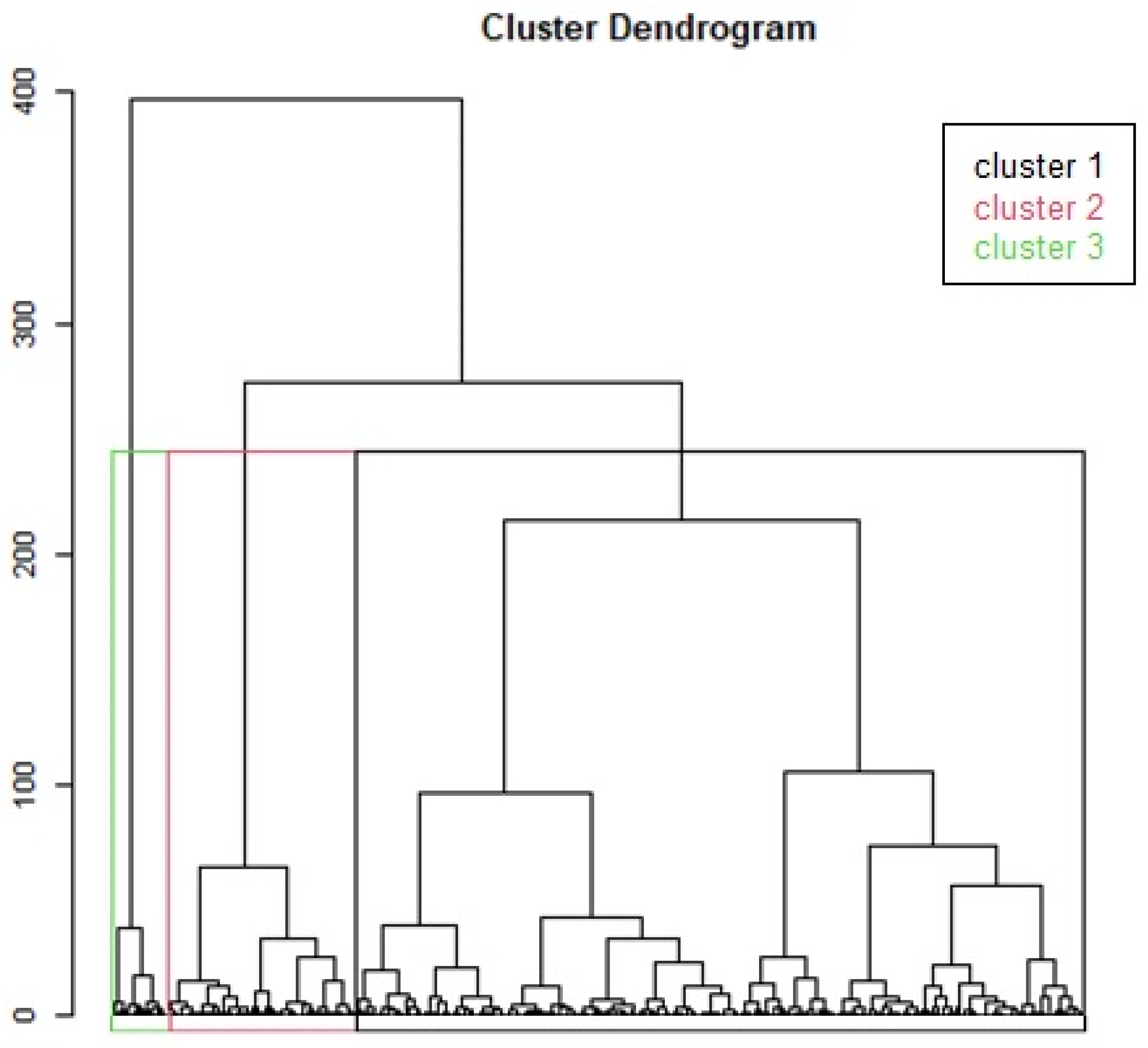
In this case, the classification of the four groups showed that these individuals could be grouped somewhat more closely because they were nearer to each other and probably quite similar internally. This was especially true for clusters 1 and 3, where a new mixed cluster group was generated in order to reduce to the maximum (optimum) number of final clusters. Figure 1 shows the hierarchical tree formed by the three new clusters (K = 3 is optimal), which are more homogeneous within the same profile group and more heterogeneous among themselves, which makes it easier to interpret the final profiles generated.

In contrast, as there is no additional information available for the optimal number of groups K (except that which was extracted using PCA, where there could be four groups, and the one reflected in the visual support of AC analysis, with three possible groups), the K-means algorithm was applied for a range of K values. The K value was thus changed to 20, 15, 10, and even 5 for the different methods. However, this was performed only for the two best cluster methods, depending on the cophenetic coefficient, Simple and Average. The goal was to identify that value from which the reduction in the total sum of intra-cluster variance was no longer substantial. For this purpose, we applied the Elbow strategy or method, with the function “fviz_nbclust” of the R package factoextra [28], which automates this process and generates a representation of the results that help to detect the inflection point of change. This facilitated the selection of the most effective number of clusters.

Therefore, the visual results of the K-means and the correlation coefficients showed that the best method was simple linkage (defined by clustering 2) of minimum distance, with 76.5%, which was composed of four groups. This indicated the possibility of generating a classification with an optimal number (K) of fewer than four groups. Similarly, final analysis revealed that the optimal number ranged from five to three clusters of groups. This signified that the number of clusters could be optimized to three cluster profiles.

Accordingly, the number of groups (clusters) was obtained by determining the optimal value (profiles) on the basis of criteria such as the Silhouette, Elbow, and Calinski–Harabasz methods or the K-means algorithm, which confirmed this final division value for different risk levels. To evaluate the classification performance, we used quality and accuracy metrics (with cut-offs greater than 0.80) to assess the clinical usefulness of the model.

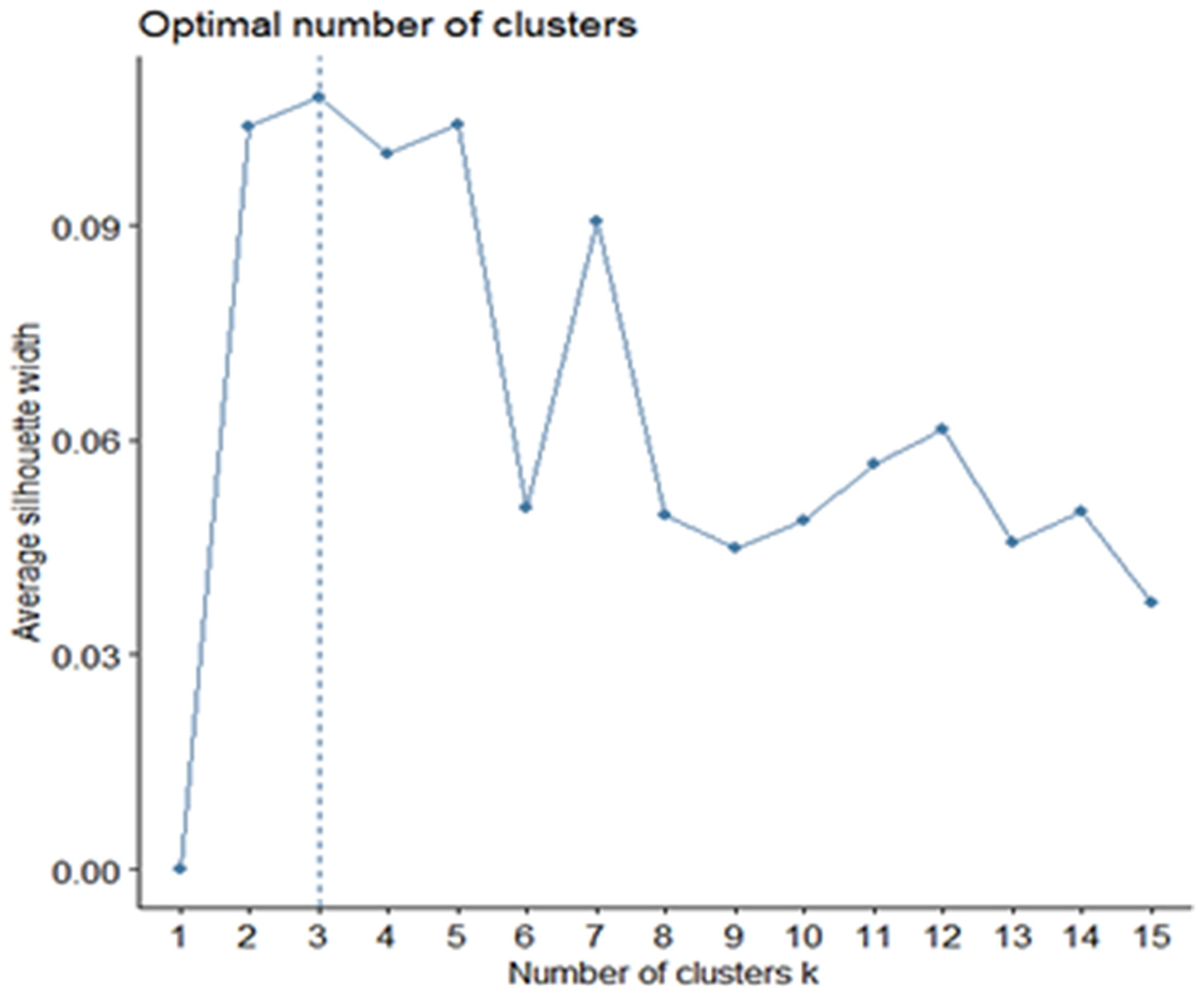
In view of these data (K-means algorithm and Elbow method), a second method called Silhouette was applied to verify the results. Although Silhouette is very similar to Elbow, the difference lies in the fact that the average of the coefficients or Silhouette indices of all the observations of individuals is maximized (Figure 2). Therefore, the results obtained from the Silhouette curve show a definitive number of three optimal clusters representing the best separation of the data, which reaffirms what was already visualized in the previous outputs.

Finally, after also exploring CA, which is described as follows, we visualized the three output clusters of groups based on our results, as well as their high and low correlation levels in the optimal clusters generated of the variables representing the characteristics of individuals (

Table 1. Correlational description of final optimal vs. variable clusters.

Variables	Cluster 1	Cluster 2	Cluster 3
CCVSDM	0.734	−2.12	2.22
DUR_ADM	2.34	−2.45	−0.203
AGE	−1.48	−1.41	5.15
SPIROMETRY_PA	5.04	2.51	−13.6
VD	0.227	−1.74	2.52
HR	−12.8	15.5	−2.54
FEV1P	−11.9	−0.992	23.9
FEVFVC	−24.3	−1.03	46.9
RR	−1.28	2.18	−1.31
FVCP	9.46	−0.63	−16.5
SMOKING_HABIT	2.96	−0.112	−5.32
CVD	−0.334	−2.35	4.6
CHF	−0.114	−1.38	2.54
BMI	1.84	−3	1.66
DEATH_90DAYS	1.69	−2.37	0.873
WKG	2.51	−3.77	1.72
VS	−0.936	2.2	−1.98
DBP	−26.7	30.8	−2.62
SBP	−40.3	44.4	−0.136

and Glossary). In this case, the sample comprised 5178 hospitalized patients suffering from an exacerbation of Chronic Obstructive Pulmonary Disease (eCOPD). The analysis of this sample was based on the differences in the stages and progression of disease, clinical pathologies, and the characteristics of the patients, which were extremely diverse.

The classification of the three groups of optimal profiles is described as follows.

Cluster 1 was formed by patients with high values for the following variables (in descending order from the highest): Spirometry FVC in % of theoretical (FVCP), Spirometry performed prior to admission or at discharge (SPIROMETRY_PA), Tobacco Habit (SMOKING_HABIT), Weight (WKG), and Duration of Hospital Admission (DUR_ADM). These patients also had low values for the following variables (in ascending order from the lowest): Systolic Blood Pressure (SBP), Diastolic Blood Pressure (DBP), Relational Ratio FEV1/FVC previous or discharge spirometry (FEVCVF), Heart Rate (HR), and FEV1 spirometry in % of theoretical (FEV1P).

Cluster 2 was formed by patients with high values for the following variables: Systolic Blood Pressure (SBP), Diastolic Blood Pressure (DBP), Heart Rate (HR), Spirometry performed prior to admission or at discharge (SPIROMETRY_PA), Ventilatory Support (VS), and Respiratory Rate (RR). These patients also had low values for the following variables: Weight (WKG), Body Mass Index (BMI), Duration of Hospital Admission (DUR_ADM), Deaths at 90 days (DEATH_90DAYS), Cerebrovascular Disease (CVD), and Cardiovascular Comorbidity (CCVSDM).

Cluster 3 was formed by patients with high values for the following variables: FEV1/FVC ratio spirometry prior to admission or discharge (FEVCVF), FEV1 spirometry in % of theoretical (FEV1P), AGE, Cerebrovascular Disease (CVD), Congestive Heart Failure (CHF), Vascular Disease (VD) and Cardiovascular Comorbidity (CCVSDM). They also had low values for the following variables: Spirometric FVC in % of theoretical (FVCP), Spirometry performed prior to admission or at discharge (SPIROMETRIA_PA_), Tobacco Habit (SMOKING_HABIT), Diastolic Blood Pressure (DBP), Heart Rate (HR), and Ventilatory Support (VS).

3.2. Correspondence Analysis

The Correspondence Analysis package “ca” [29] was used as a part of the main analysis (Cluster) to complete the result of the classification in groups. This visually descriptive multivariate technique represents the relationship between variables using an association measure in a low-dimensional space with the least possible loss of information [30,31]. In other words, it is a dimension reduction method, equivalent to PCA, Factor (FA) and Discriminant (DA) analysis for categorical, nominal or ordinal variables. It thus helps to visualize the multidimensional point cloud in two dimensions.

CA shows that the inertia of the first dimensions indicate whether there were strong relationships between the variables and suggest the number of dimensions that need to be studied, which provided additional support for our exploration.

Based on the results in

Table 2. Decomposition of total inertia using CA. Eigenvalues for Dim.1–Dim.31.

	Dim.1	Dim.2	Dim.3	Dim.4	Dim.5	Dim.6	Dim.7	Dim.8	Dim.9
Variance	0.018	0.010	0.008	0.006	0.005	0.004	0.003	0.003	0.002
% of var.	24.132	14.053	11.038	8.358	7.037	4.832	3.713	3.485	3.145
Cumulative % of var.	24.132	38.185	49.223	57.581	64.618	69.449	73.162	76.647	79.792
	Dim.10	Dim.11	Dim.12	Dim.13	Dim.14	Dim.15	Dim.16	Dim.17	Dim.18
Variance	0.002	0.001	0.001	0.001	0.001	0.001	0.001	0.001	0.001
% of var.	2.415	1.896	1.723	1.669	1.608	1.520	1.491	1.370	1.307
Cumulative % of var.	82.206	84.103	85.826	87.495	89.104	90.624	92.115	93.485	94.792
	Dim.19	Dim.20	Dim.21	Dim.22	Dim.23	Dim.24	Dim.25	Dim.26	Dim.27
Variance	0.001	0.001	0.001	0.000	0.000	0.000	0.000	0.000	0.000
% of var.	1.204	1.040	0.813	0.621	0.331	0.290	0.273	0.239	0.211
Cumulative % of var.	95.996	97.036	97.849	98.470	98.801	99.091	99.364	99.603	99.814
	Dim.28	Dim.29	Dim.30	Dim.31
Variance	0.000	0.000	0.000	0.000
% of var.	0.084	0.073	0.027	0.002
Cumulative % of var.	99.898	99.971	99.998	100.000

, the first two dimensions expressed 38.19% of the total inertia of the dataset. This means that the total variability in the row (or column) cloud is explained by the 1:2 plane. Obviously, this is an intermediate, though substantial, percentage for these data. The first plane represents a part of the variability in the data, which is much larger than the reference value (7.45% equal to the 95th percentile of the distribution of inertia percentages obtained by simulating 101 tables of data of equivalent size on the basis of a uniform distribution). Based on these figures, the variability explained by this plane is very important.

In consonance with PCA and in the event that better results are needed, the dimensions that also express a high percentage of the total inertia could be considered. This would mean interpreting those greater than or equal to the third to complete the information.

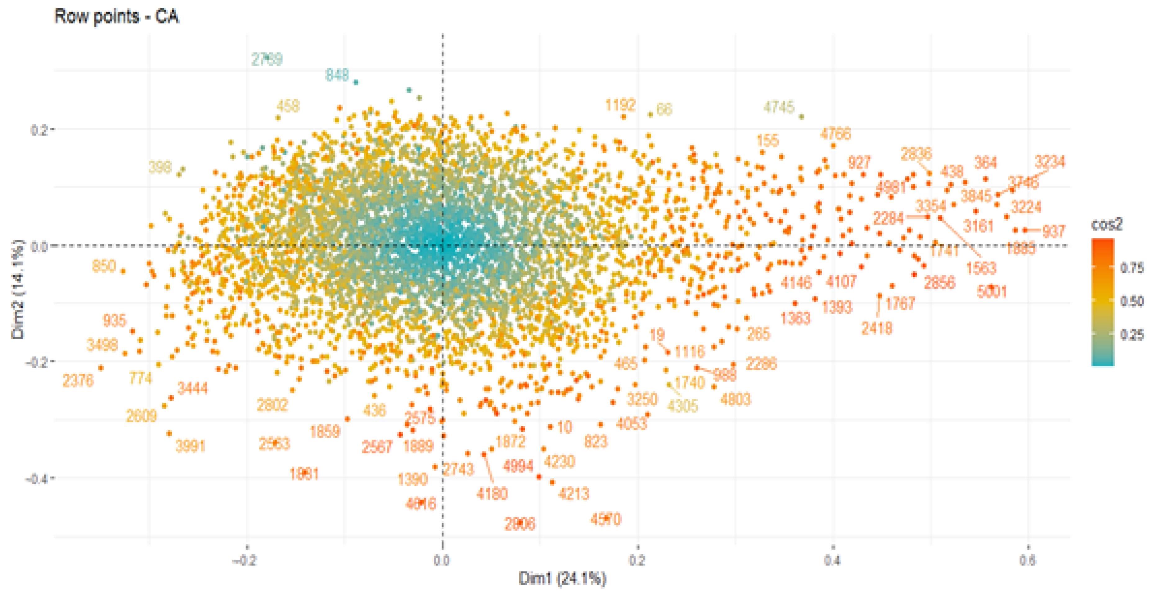
The CA results indicated that an estimate of the correct number of axes to interpret should restrict the analysis to the description of the first eight axes, especially since they carry the vast majority of real information. They also showed an amount of inertia 76.65% higher than that obtained by the 95th percentile of random distributions (28.61%). The most relevant description was found to be located on these axes, the first two of which contribute more to the total inertia. More specifically, the contribution of the first axis was 24.13%, whereas that of the second one was 14.05%.

As confirmation, these axes can be visualized on a sedimentation graph. This is another way of viewing the correct final axes, along with which the optimal number of components is shown. Since the values above point 1.0 were the most acceptable, this verified that the eight previous components (eigenvalues greater than one) were still the ones with the majority of the valid information. The red dashed line of the screen plot also indicates what the contribution would be (in terms of the percentage of variability in each dimension) if they were homogeneous.

In addition, this describes dimensional contributions in the 1: 2 plane for the different variables (columns) in order of importance on the axis. As reflected, there are three variables with a high percentage of contribution to the axis. There are also two more variables (just the cut of the dashed line) with a lower percentage of contribution to the plane. However, they must also be taken into account in the analysis of this axis (1–2), as well as the rest of variables with less weight, but with the same relevance.

In parallel, a matrix of correlations between variables (strong–weak) was also visualized in the analysis outputs. This ensured that these were high as one of the fundamental requirements. This was achieved by dimensionally representing the contribution of each attribute variable on each axis, especially the 1:2 plane, and by highlighting dimensions 3 and 5, given their importance and despite their complex description.

Based on the results obtained with the different methods, the optimum number of groups was found in three profiles, which verified the outputs of cluster analysis.

As this procedure was an additional support for the main analysis (Cluster), we visualized the results on the 1:2 plane and the representations, both separately and as a whole, for the patients (Figure 3) and variables (cols). This revealed that the three groups were generated by similar characteristics within the same profile (patients or variables), as reflected by the degree of the color scale. In addition, there were factors of patients which were closely correlated and which summarized this axis (correlation quite close to 0.97).

3.3. Decision Tree Classification Analysis

As part of our search for optimal profiles, we also explored Decision Tree (DT) classification analysis [32,33,34] as another way to support the main analysis (Cluster). This analysis was performed to detect any relevant information or classifications hidden among the optimal clusters that could improve the final clustering result generated by the three groups of final profiles.

The Decision Tree (DT) method from R’s rpart package [21] is a supervised learning technique. It is similar to Support Vector Analysis (SVM), where both supervisory algorithms are based on the classification (or regression) of previously labeled data. The idea was to find the relationships between them using a function, which associated the input variables with the output variables to generate a decision tree able classify or predict the observations of individuals in the future [35,36].

DT differ from unsupervised procedures, such as Cluster analysis, CA, and PCA, which describe and find data structures that either define groups based on their similarity (distance) or simplify them to maintain their essential characteristics, and thus increase the quality of the data by improving the performance of these algorithms.

Decision Trees [37,38,39] are one of the most powerful algorithmic approaches currently used in the vast majority of Machine Learning research fields, especially in the fields of healthcare and data mining or data science, which search for different behaviors that can define efficient and more accurate sets of patterns, that are applicable to the general population.

This classification algorithm uses simple decision rules or dichotomous constraints, which are usually composed of two groups or classes as a part of its classificatory analysis. It maintains a hierarchical order in its application and builds a tree structure to represent it visually as a final result. This aids decision making by describing the data without determining the final resolution of them [8,40].

However, this process only keeps the attributes or categories that matter in decision making and discards those attributes that do not contribute to the accuracy of the tree. This information is thus of great value and can be used to reduce the data to the most important variables before applying another technique.

Given their accuracy and security, decision tree models are now widespread and are frequently used in many research fields since they are a simple, self-explanatory, and easily scalable technique. They can handle a wide variety of different input data variables with a minimal computational cost. Moreover, they are able to process datasets with missing values, which results in high predictive power with little computational effort. In fact, they can even handle noisy data using internal mechanisms (such as “pruning”) that reduce the depth of the tree in such a way as to obtain the best generalization. They can also support different functions depending on the objective, either for classification, regression, or clustering. Finally, they are also an additional technique for the variable (or category) selection procedure in the final screening of attributes (or variables).

Nevertheless, the DT method has certain limitations. Firstly, when a high-depth factor is applied, it may present problems of overlearning, which complicates the algorithmic process on the class categories. Secondly, it does not detect correlations between the variables, since each decision node is obtained independently, without taking into account the rest of the nodes or tests.

However, the Decision Tree (DT) technique was used in our study as an additional exploratory classification support in the search for patient profiles and to detect any changes in the data that might improve the final definition of the profile groups. That said, various cases (classes) were explored. Although only two of them were of clinical interest, they could provide valuable information pertaining to hospital admissions and smoking, offer an extra result, or simply confirm the existing data.

This procedure was started by setting a seed (“seed = 500”), which was subsequently varied (seed = 1000 or 1500) in order to detect significant changes. This function (seed), which is a number (or vector), was used to initialize the pseudo-random number generator, which helped to make the results of the models reproducible elsewhere. Furthermore, the dataset was divided into two parts, where 70% were training data and 30% were test data for the subsequent validation of the results obtained.

In this context and in view of the results of the first decision tree on smoking data, it was observed that 82% of the patients were smokers. Classification thus started with the gender variable (sex labeled as (1) female or (0) male) in the first section of the decision flow and ended with a spirometric test and an advanced age cut-off. This tree (whose visual presentation was quite blurry) concluded by showing the following results: (i) 12% of female smokers over 73 years of age (6%) had a predisposition to severity of 6%; and (ii) 88% of male smokers without spirometry performed (27%) had a predisposition to severity of 60%.

Unfortunately, this mapping problem is very common when the tree has a greater depth. This makes its decision rules more complicated, which leads to a very unclear tree structure.

As in the previous case, the results of the second decision tree on the hospital admission data showed that 35% of the patients underwent hospital admission. The classification started with the exacerbation readmission variable (labeled (1) Yes or (0) No) in the first leg of the decision flow and ended with a three-month mortality event check.

Even though the visual representation of this other tree was not very clean, it reflected conclusive results that should be taken into consideration, such as the following: (i) out of 73% of the patients not readmitted for exacerbation, only 2% were predisposed to die; and (ii) 27% of the patients who were readmitted died within 90 days of readmission for exacerbation because of the severity of the disease itself and repeated hospital readmissions without improvement after the recommended therapies.

4. Discussion

Based on the results obtained, cluster analysis was found to be a good choice since it is one of the best methods for data representation when it is a question of dividing groups that are homogeneous within themselves and which are heterogeneous among themselves. In our study, this technique obtained an optimal final result of three groups of clinical profiles, which were both different from each other and similar with related characteristics. This achieved our initial objective, which was to identify patterns of related profiles in order to classify the patients into groups with the same behavior. In this way, their properties or characteristics could be studied in detail, with a view to improving their clinical treatment and care and to extrapolating the results and conclusions of our study to the general population.

For this purpose, different techniques were analyzed for the description and visual representation of the data collected. In a parallel way, different metrics were also implemented to compare the results obtained, and at the same time, to select the best strategy to obtain high-quality information. The goal was to implement different dimensional reduction techniques without the loss of valuable data. We also wished to identify an effective algorithm for the creation of different groups in order to obtain optimal clinical profiles.

Correspondence Analysis (CA) and Decision Analysis (DA) were also used as an additional part of the exploration because they provided a visual complement that profiled and adjusted the information obtained. They also allowed us to confirm that the optimal final result of the grouping was the right one, which verified our initial hypothesis.

As a result, the cluster analysis in our study obtained an optimal number of clusters of several grouped profiles of patients with similar characteristics. All of them have closely interrelated variables with sufficient relevance to be considered in each clinical profile. More specifically, these three group profiles are based on the following details, which point to three levels of severity in the individual.

Profile 1 represents a group of patients who were smokers with relevant spirometric data and problems with diet, blood pressure, and heart rate values, which could also cause long-term hospital stays (i.e., variables FVCP, SPIROMETRY_PA, SMOKING_HABIT, WKG, DUR_ADM, SBP, DBP, FEVFVC, HR and FEV1P). All of this aggravated and worsened the conditions of the patients, who were weakened by other pathologies in addition to the main one.

Profile 2 represents a group of hypertense patients with spirometry performed and varying spirometric data. These patients possibly needed ventilatory support due to comorbidities, including a history of a cerebral vascular event, weight-related dietary problems, and long-term hospital stays conducive to a short-term negative outcome (i.e., variables SBP, DBP, HR, ESPIROMETRY_PA_, VS, RR, WKG, BMI, DUR_ADM, DEATH_90DAYS, CVD and CCVSDM). The recommendation was for them to adopt healthy habits that could improve their quality of life until the final stage of life and lessen the general wear-and-tear caused by other pathologies in addition to the central one.

Profile 3 represents a group of fairly severe patients with various comorbidities and pathologies (i.e., cerebrovascular event and congestive heart failure), with variable spirometric and anthropometric values due to their advanced age. These patients, who are probably hypertensive, as well as smokers, have ventilatory support needs because of cardiovascular comorbidities, (i.e., variables FEVFVC, FEV1P, AGE, CVD, CHF, VD, CCVSDM, FVCP, SPIROMETRY_PA, SMOKING_HABIT, DBP, HR and VS). Their condition rapidly worsened because of the main pathology and therapies. This means that other alternatives should be reviewed to maintain a good quality of life.

However, these results are not clinically conclusive since all the algorithms have certain limitations and may need to be complemented with other techniques if these models are to be reproduced in different settings with the same approach.

The results of this study provide new insights into the relevant factors (i.e., final clinical variables) for this type of patient. However, since they are separated into three levels of severity, efforts and knowledge should be focused on devising clinical procedures and treatments that will improve their diagnoses and their quality of life over time.

5. Conclusions

This research study showed that it is possible to use a set of classification techniques to analyze situations characterized by a sufficiently large volume of data. In this particular case, the cluster groups showed very similar clinical characteristics. This signified that the development of other pathologies (i.e., chronic diseases) with irregular increases in vital signs and frequent hospital admissions was caused by the severity of the disease itself and the advanced age of these patients, combined with poor health habits and their COPD exacerbations. This meant that the clinical condition of these patients was severe and would progressively deteriorate over time.

In this sense, our research study showed the usefulness of computational methods of supervised and unsupervised learning to facilitate the search for patterns in high-dimensional datasets coming from multicenter studies or Big Data repositories. In such contexts, it is almost always necessary to apply a classification procedure by clustering, which can add value to the clinical variables collected by professionals. However, before applying any algorithm, it is necessary to perform a filtering mechanism to select the most relevant variables or data in order to give validity to the decision.

Moreover, in many cases, this additional information is needed to make the correct diagnoses and, at the same time, personalize the procedures and treatments that do not require so many clinical resources. This leaves more time for people to improve their health habits, which provide a better quality of life.