
Geometric Loci and ChatGPT: Caveat Emptor! †

1
Departamento de Matemática Aplicada I, University of Vigo, 36005 Pontevedra, Spain
2
Departamento de Ingeniería Industrial, Escuela Politécnica, University Antonio de Nebrija, 28040 Madrid, Spain
*
Author to whom correspondence should be addressed.
†
Computation 2024, 12(2), 30; https://doi.org/10.3390/computation12020030
Submission received: 6 December 2023
/
Revised: 30 January 2024
/
Accepted: 5 February 2024
/
Published: 7 February 2024
Abstract
:We compare the performance of two systems, ChatGPT 3.5 and GeoGebra 5, in a restricted, but quite relevant, benchmark from the realm of classical geometry: the determination of geometric loci, focusing, in particular, on the computation of envelopes of families of plane curves. In order to study the loci calculation abilities of ChatGPT, we begin by entering an informal description of a geometric construction involving a locus or an envelope and then we ask ChatGPT to compute its equation. The chatbot fails in most situations, showing that it is not mature enough to deal with the subject. Then, the same constructions are also approached through the automated reasoning tools implemented in the dynamic geometry program, GeoGebra Discovery, which successfully resolves most of them. Furthermore, although ChatGPT is able to write general computer code, it cannot currently output that of GeoGebra. Thus, we consider describing a simple method for ChatGPT to generate GeoGebra constructions. Finally, in case GeoGebra fails, or gives an incorrect solution, we refer to the need for improved computer algebra algorithms to solve the loci/envelope constructions. Other than exhibiting the current problematic performance of the involved programs in this geometric context, our comparison aims to show the relevance and benefits of analyzing the interaction between them.
1. Introduction
Large Language Models (LLM) [1] have attracted a lot of attention in recent times. A LLM known as ChatGPT [2] was released at the end of 2022, and its accuracy has been rapidly tested in different fields of knowledge [3,4,5,6,7,8,9], given its question-and-answer dialogue procedure. Mass media were primarily concerned with plagiarism and student cheating (see, for instance, [10,11]). Concerning interaction mathematics and ChatGPT, various studies have been reported. For instance, in [12] the authors investigate the mathematical capabilities of ChatGPT on standard and ad hoc datasets; mathematical word problems are considered in [13]; and an extensive list of ChatGPT failures, related to mathematics and other issues, is given in [14], to mention just a few references on this interplay.
Some renowned authors [15] stated that these machine learning programs cannot really replicate human understanding, and conclude that
ChatGPT and its brethren are constitutionally unable to balance creativity with constraint. They either overgenerate (producing both truths and falsehoods, endorsing ethical and unethical decisions alike) or undergenerate (exhibiting noncommitment to any decisions and indifference to consequences). Given the amorality, faux science and linguistic incompetence of these systems, we can only laugh or cry at their popularity.
Moreover, although, at the time of writing issues, such as privacy and the need for state regulations involving AI tools, are being discussed, no severe objections are posed regarding the use of ChatGPT in mathematics, to the best of our knowledge. Indeed, the main developer of Mathematica wrote a laudatory welcome to the chatbot [16], announcing a Wolfram|Alpha plugin for ChatGPT. It is highly arguable that we should rely on hidden proprietary codes to perform computations in mathematics, as stated by J. Neubüser, the developer of GAP (cited in [17]).
With this situation two of the most basic rules of conduct in mathematics are violated: in mathematics, information is passed on free of charge, and everything is laid open for checking.
ChatGPT has also attracted a lot of attention from the education field. A review [18] found that fifty related scholarly articles written in English were published in January and February of 2023 alone, and concludes that the chatbot’s performance is unsatisfactory in mathematics education. A very commendable article [19] on ChatGPT and mathematical education, although recognizing the existence of contrary opinions, states that “ChatGPT lacks a deep understanding of geometry and cannot effectively correct misconceptions”. We will not discuss the machine understanding issue, which would lead us to a philosophical debate involving the Turing Imitation Game. Despite these negative precedents, we think—and will exemplify in this paper—that exploring a specific geometric issue (and this should be actually considered the key contribution of the program: to help humans to explore, not to fully replace human inquiry) with ChatGPT will promote the expansion of our geometric knowledge.
Indeed, this argument is not new. The emergence of chatbots in the field of mathematics can be seen as somewhat similar to the introduction of symbolic calculation programs. It is worth noting a couple of works that dealt with the topic at the end of the 20th century. In one of them, a founder and leader of this area, Buchberger, presents [20] a didactical principle, the White-Box/Black-Box Principle for Using Symbolic Computation Software in Math Education, stating that, when a mathematics topic is new to students, the use of symbolic software should be prohibited; when it has been thoroughly studied and hand calculations involving concepts from such topics have been made, “students should be allowed and encouraged to use the respective algorithms available in the symbolic software systems”. Similarly, the recommendation given in [21] is that, prior to using symbolic computation software, students should thoroughly study the main theoretical issues in the topic under consideration and resolve related problems by hand (in order to keep fundamental mathematical operations and skills). They conclude with two rules of thumb that we summarize as follows:
- If you know how to do it, use computer algebra. If not, do not use it.
- Caveat emptor!
It is from this educational perspective, and with the aim of contributing to the exploration of the mathematical abilities and shortcomings of ChatGPT, that we study its performance in dealing with a few (but representative for their presence in the curriculum or in some recent research papers (see references below)) plane geometric loci and envelopes of families of plane curves, a popular topic both in the educational and mathematical research contexts. We remark that the issue of loci and envelopes, while thoroughly studied either from a theoretical point of view [22,23,24], or within the context of dynamic geometry systems [25,26,27,28], has not been approached, as far as we know, with AI chatbots. It is true that LLMs have been tested in relation to formal theorem proving in Euclidean geometry (see, for instance [29,30]), but the topic of the algorithmic computation of loci/envelopes is not, technically speaking, part of the theories addressing the automated deduction of theorems in geometry. Computing loci/envelopes concerns, rather, finding some missing necessary conditions (the description of the locus of a point as the result of establishing some given constraints over that point).
In our experiment, we used the free 3.5 version of ChatGPT from 25 September 2023. Some elementary, albeit non trivial, loci constructions were posed to the chatbot, and its results are discussed and compared with those obtained with a fork version of the popular, free dynamic geometry program GeoGebra [31], called GeoGebra Discovery, which includes rigorous automated reasoning tools based on computational algebraic geometry algorithms implemented in Tarski 1.30 and Giac, two embedded computer algebra systems [32,33,34,35]. In the case were GeoGebra Discovery does not give the right solution, we provide a specific analysis of the situation, describing the need for implementing improved computer algebra algorithms.
We envisage two types of users when searching for geometric loci and envelopes either with ChatGPT or GeoGebra, mainly the undergraduate, or even secondary education student, faced with a proposed task in these issues. Secondarily, we envisage researchers in other fields with collateral tasks involving these geometric problems. So, the need for free access, either to ChatGPT (via its webpage) or to GeoGebra (downloading this free, multi-platform program), is a prerequisite in this work.
It should be highlighted that only the web-accessible ChatGPT page, https://chat.openai.com/ accessed on 6 December 2023, will be used throughout this paper. Thus, we specifically exclude considering others LLMs, as well as, concerning ChatGPT, experimenting with variations in temperature and top-p parameters. We also refrain from considering related ChatGPT prompting techniques, such as few-shot learning, tuning, and chain-of-thoughts, with the exception of the construction in Section 2.1. The rationale behind our decision is two-fold: on the one hand, fine tuning the model would require accessing the GPT-3 API, which might involve costs, thus losing the required characteristic of being free of charge. On the other hand, while maintaining prolonged dialogues with the chatbot could be illuminating, it could also be frustrating for a student, as well as a possible new source of errors, as shown in the construction in Section 2.1.
Next, Section 2 describes some geometric loci with both systems and provides an “ad hoc” ChatGPT-assisted procedure for suggesting how the user can input a GeoGebra locus construction. Section 3 considers some envelopes and discusses their solutions using, again, both systems. Finally, we conclude, analyzing the behavior of this collection of representative cases, that ChatGPT is not mature enough for us to rely only on its use, and we point to some ways teachers can guide learners when using the chatbot for these geometric problems.
2. Geometric Loci
A classic problem in plane Euclidean geometry consists in finding the path of an construction element that is subject to given constraints. In cases where the element is a point, we call the problem a “geometric locus”. The usual difficulties when mentally visualizing various objects with different movements lead to the use of computer software allowing for the graphical visualization of loci, mainly dynamic geometry software. Besides the graphical representation of loci, we obtain full knowledge of such loci when finding their analytical description. Thus, although ChatGPT does not currently have sophisticated graphic abilities, we study its competence when finding the analytic determination of loci.
2.1. Simple Geometric Loci
ChatGPT correctly identifies simple loci as circles and ellipses. For instance, when asked “Find the locus of plane points equidistant, say 1, from one given, say A(0, 0)”, it finds the equation and states it is a circle centered at the origin with a radius of 1. Similarly, when asked about “Find(ing) the locus of points which sum of distances to a pair of given points is constant”, it returns “The locus of points in a plane such that the sum of their distances to two fixed points (called foci) is constant forms an ellipse”, and, since no particular coordinates nor distances are given, the found equation is , with obvious coordinate assignments.
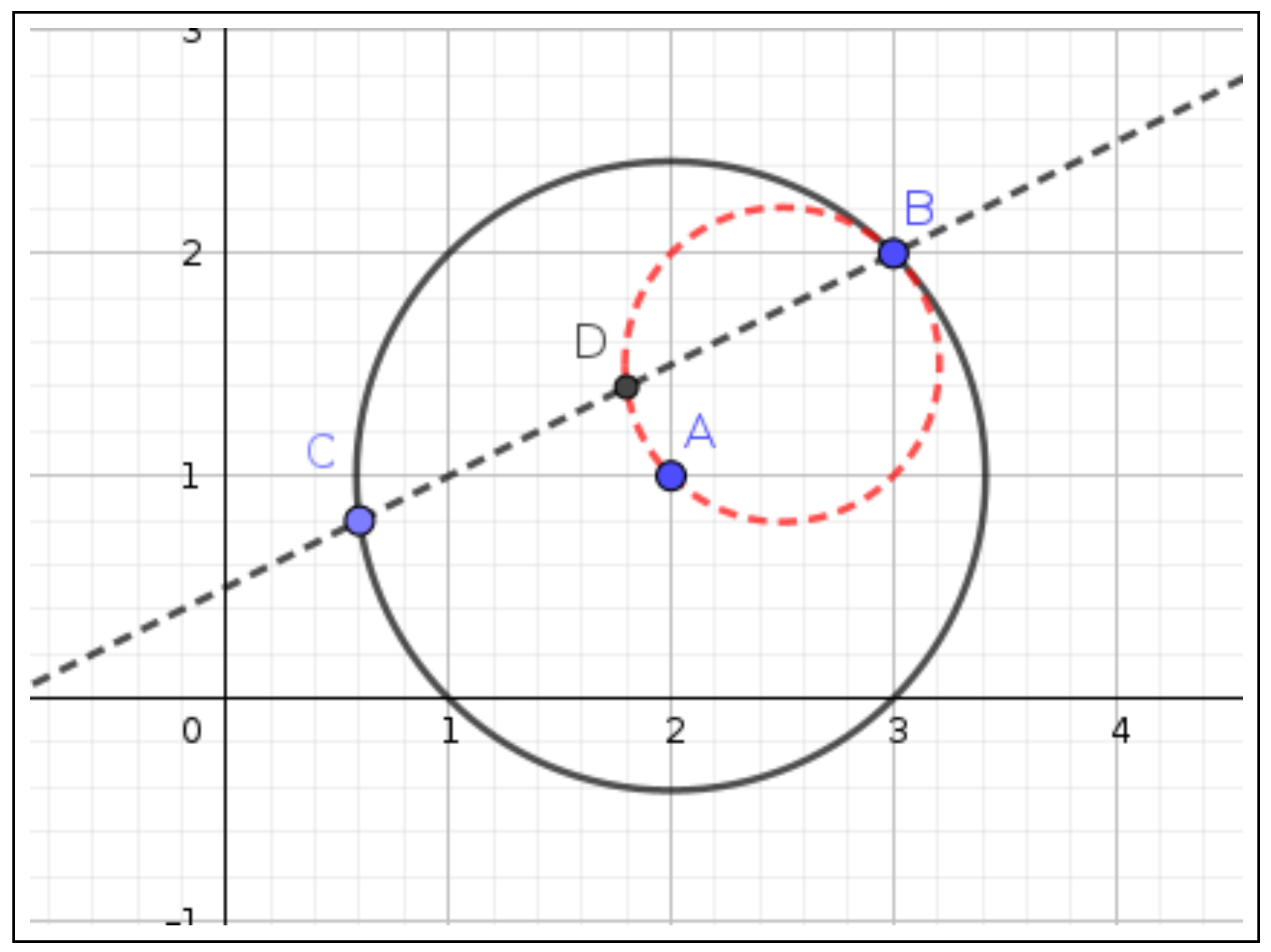
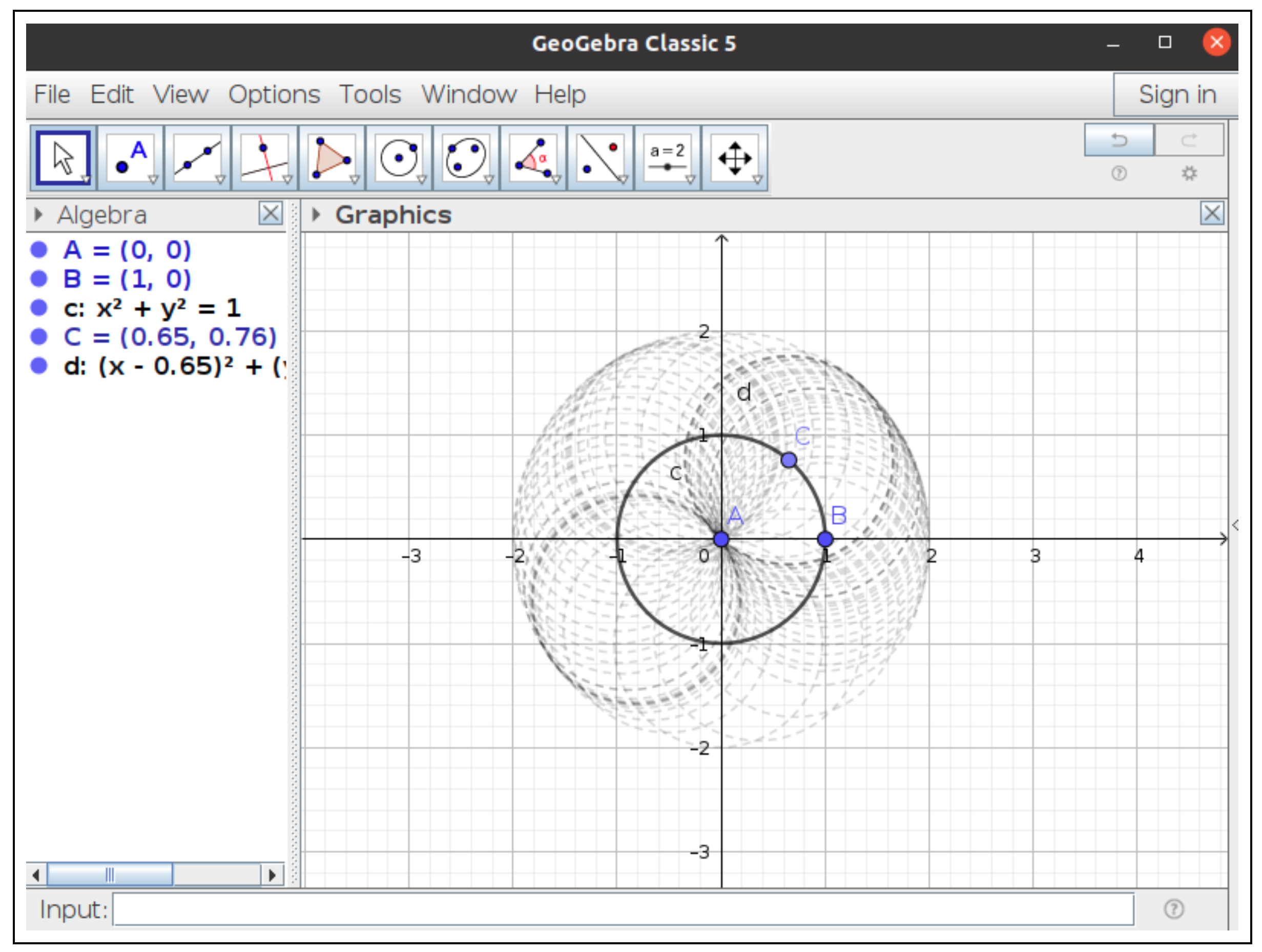
Nevertheless, ChatGPT does not give an accurate answer, at a first sight, to the following simple construction (a graphical representation made with GeoGebra is shown in Figure 1, suggesting that the sought locus is a circle):
- Question Consider a circle centered at and passing through . Place a moving point in this circle, C, join it with B and compute the midpoint D of . What is the geometric locus of D?
- ChatGPT Let us denote the center of the circle as , and a point moving on the circle as . Since C lies on the circle passing through , the distance between A and C is equal to the radius of the circle.
The distance formula between two points and is given by
For and on the circle, the distance is equal to the radius of the circle. Let r be the radius:
Now, we want to find the midpoint D of the line segment , where is the other endpoint of . The midpoint D is given by the average of the coordinates of B and C:
Substitute the expression for r from the equation of the circle into the coordinates of C to obtain the coordinates of D:
Now, substitute the expression for r into the coordinates of D:
Now, you have the coordinates of the midpoint D in terms of the variables x and y. If you simplify further, you might find a specific geometric shape for the locus of D, but the exact form depends on the simplification of the expression.
The computations are correct, although the last substitution is fruitless. Furthermore, eliminating the coordinates of C, in the following equations,
the chatbot would obtain the sought locus. Nevertheless, no clue about the locus is given. Let us follow the advice on further simplification:
- Question Simplify the expression.
- ChatGPT Let us simplify the expression for the coordinates of the midpoint D:
Now, we know that , so substitute this into the coordinates of D:
Now, let us eliminate the denominators by multiplying both sides of the equation by 2:
Square both sides to eliminate the square root:
Expand and simplify:
Now, simplify further:
Move all terms to one side:
So, after simplifying, the geometric locus of the midpoint D is given by the following equation:
This is the equation that describes the locus of the midpoint D as the point C moves on the circle. The exact geometric shape of this locus might be evident with further analysis or manipulation.
There is a bizarre mistake in line 7 of the answer, where it is stated that , which is obviously wrong. So the locus is not the correct one. Furthermore, it should be noted that is not identified as a parabola. We need a further interaction to obtain the right result:
- Question: Eliminate x and y in the equations .
Finally, we obtain, after renaming the coordinates of D and suppressing the verbose output of ChatGPT,
ChatGPT does not have direct access to external services or computational tools, but it can help when describing GeoGebra procedural constructions. For instance,
- Question: Give a procedural description in GeoGebra’s input bar of the above construction, using the LocusEquation Command. Use the Execute command in GeoGebra to provide the description.
- ChatGPT: Certainly! Below is a procedural description for the construction using GeoGebra’s input bar. Note that GeoGebra does not have a direct Execute command, but you can input commands directly into the input bar.
- Open GeoGebra: Open the GeoGebra app on your device.
- Create Points A and B: Input in the input bar and press Enter. Input in the input bar and press Enter.
- Create the Circle: Input c = Circle(A, B) in the input bar and press Enter.
- Create a Moving Point C: Input C = PointOn[c] in the input bar and press Enter.
- Join Points B and C: Input = Line(B, C) in the input bar and press Enter.
- Compute Midpoint D: Input D = Midpoint[] in the input bar and press Enter.
- Use the LocusEquation Command: Input LocusEquation() in the input bar and press Enter. This command tells GeoGebra to create a locus equation based on the movement of point C with respect to the midpoint D, and 1 represents the constant sum of distances.
- Animate the Movement of Point C: Right-click on point C. Select “Animation Options”. Choose “Rotate” or “Translate” to make point C move around the circle.
- Observe the Locus: As point C moves around the circle, GeoGebra will dynamically display the locus of the midpoint D.
By entering these commands into the input bar, you can construct and observe the dynamic locus of the midpoint D as point C moves within the given circle in GeoGebra.
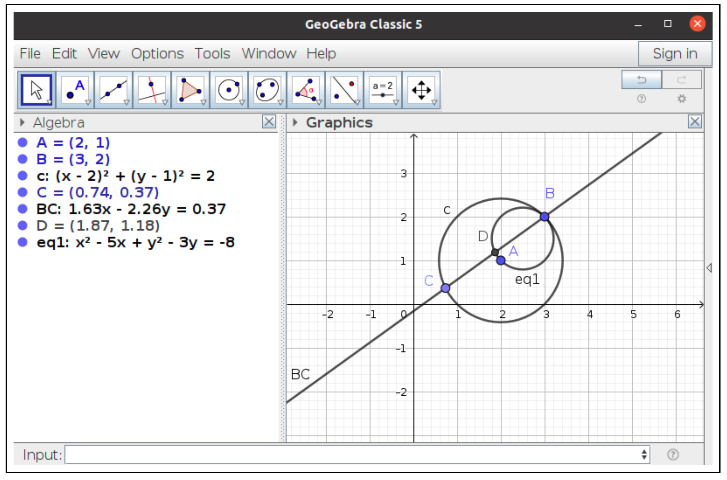
Thus, entering
Execute({"A= (2, 1)", "B = (3, 2)", "c = Circle(A, B)",
"C = Point[c]", "BC = Line(B, C)", "D = Midpoint[B,C]",
"LocusEquation(D,C)"})
- in GeoGebra returns the locus graphic object and its equation (Figure 2). There are some mistakes in ChatGPT’s translation: PointOn should be just Point, Midpoint[BC] shoul be Midpoint(B,C), and LocusEquation should only accept one or two arguments. Moreover, GeoGebra indeed has the Execute command.
2.2. The Wallace–Simson Theorem
Consider a triangle . The Wallace–Simson theorem states that the locus of all those points P is in its plane, such that the orthogonal projections of P on the three sides of the triangle are collinear is the circumcircle of . See [26] for an algorithmic, algebraic geometry, approach, and generalizations.
Despite ChatGPT knowing this statement, we will investigate this result without mentioning its name to ChatGPT. Posing the question “Consider a triangle , , , and a point P. Trace the orthogonal projections from P to the sides of the triangle. Find the locus of point P such that the orthogonal projections are collinear”, the chatbot returns the equation of a parabola, , instead of the circumcircle of the triangle. ChatGPT adequately treats the problem, but there is a calculus mistake when computing the determinant for the collinearity of points. In order to improve the readability of this paper, the trace of ChatGPT interactions will appear in an appendix from now on.
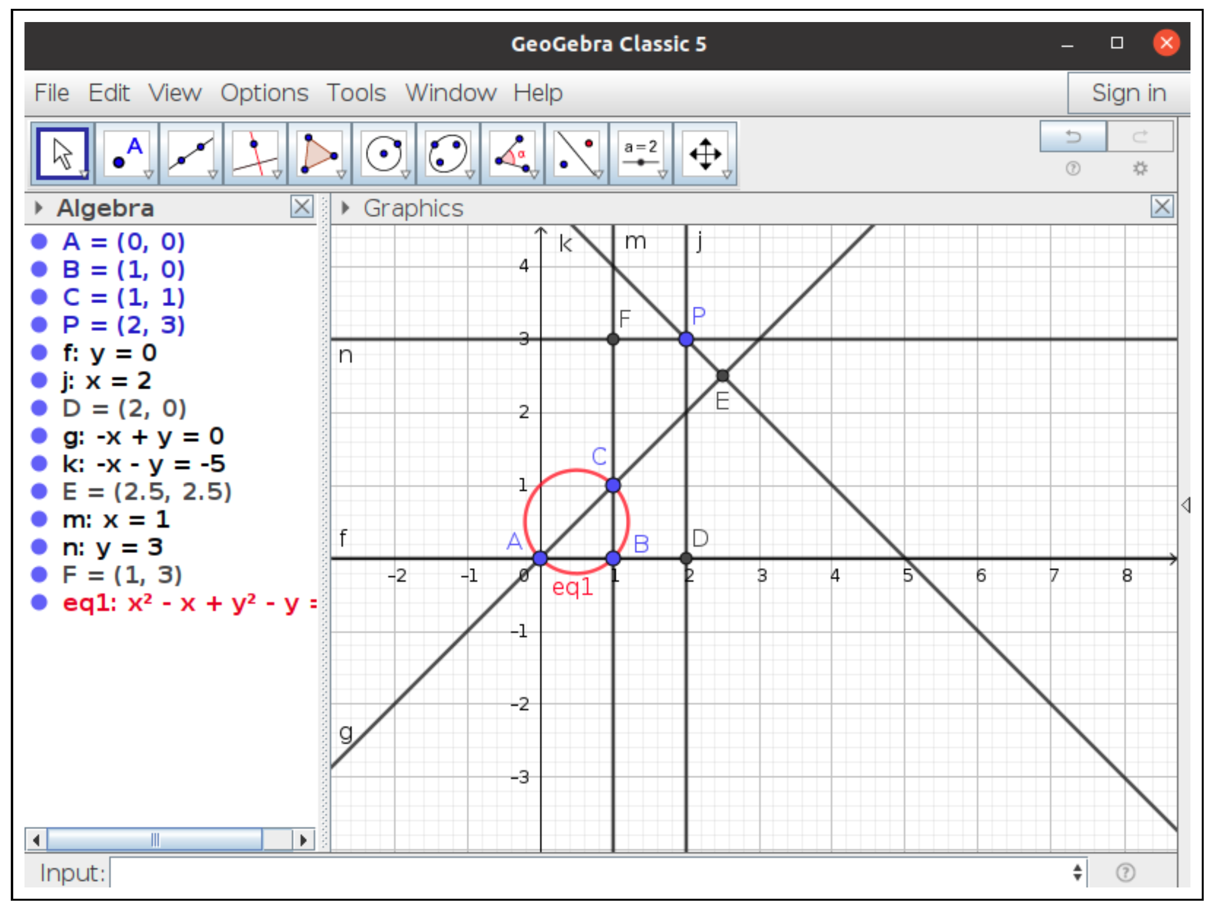
As carried out above, ChatGPT can give a procedural description of the construction (see Appendix A), which can guide a non-expert GeoGebra user to compute the locus in the dynamic software. Yet, in the current state of the art, we think it is still not worth designing a ChatGPT–GeoGebra interface for automating the translation of constructions, given the impressibility of the chatbot when curating its answers, (thus making the interface probably unuseful), and the fact that it commits frequent errors when writing GeoGebra code. Finally, entering
Execute({"A = (0, 0)","B = (1, 0)","C = (1, 1)","P = (-1,-1)",
"f = Line(A, B)", "j = PerpendicularLine(P, f)",
"D = Intersect(f, j)", "g = Line(A, C)",
"k = PerpendicularLine(P, g)", "E = Intersect(g, k)",
"m = Line(B, C)", "n = PerpendicularLine(P, m)",
"F = Intersect(m, n)", "LocusEquation(AreCollinear(D, E, F), P)"})
- into the GeoGebra input bar, we obtain the sought graphic locus and its equation (Figure 3). Note that we could not use the Locus command; since P does not lie on any known object, it is subject to an a posteriori condition.
2.3. Sketchpad Classic Locus Construction
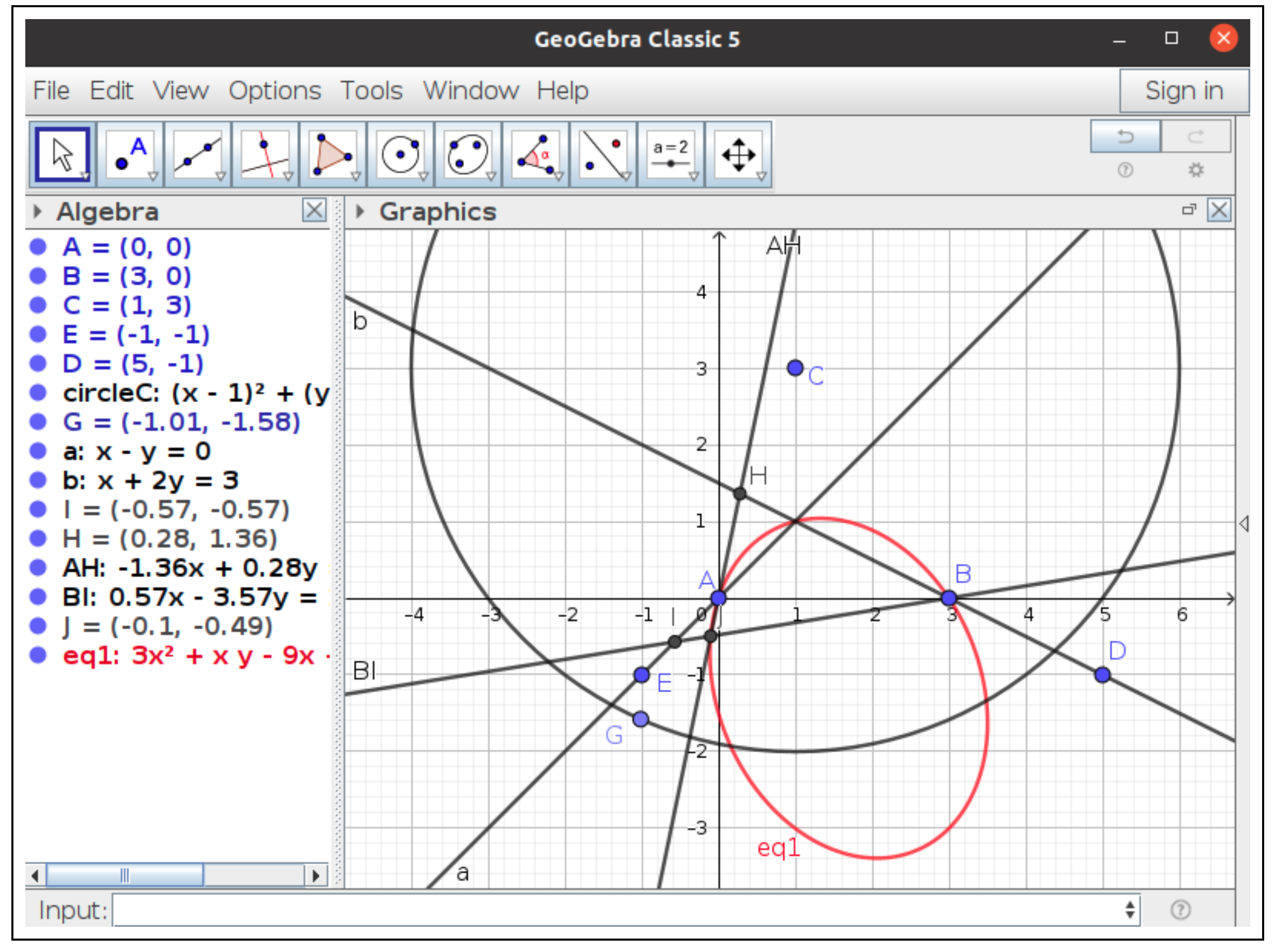
We consider a locus studied by Sutherland in his report on Sketchpad [36]. This locus is erroneously computed by ChatGPT, and GeoGebra returns an inaccurate answer. The construction can be defined as follows:
Let , and be three fixed points, and let a and b be two lines passing, respectively, through A and , and B and . Let c be the circle with center C and radius 5. Consider a moving point G on the circle c. The line intersects a in a point I and b in a point H. Find the locus of the intersection point J of lines and .
ChatGPT correctly understands the task (see Appendix B), but finds that lines and are parallel, concluding that their intersection point I does not exist. When asked about a GeoGebra procedural description, it gives a step-by-step list, assuming user familiarity with GeoGebra. With a slight change, entering
Execute({"A = (0, 0)", "B = (3, 0)", "C = (1, 3)", "E = (-1, -1)",
"D = (5, -1)", "circleC = Circle(C, 5)", "G = Point(circleC)",
"a = Line(A, E)", "b = Line(B, D)", "I = Intersect(Line(C, G), a)",
"H = Intersect(Line(C, G), b)", "AH = Line(A, H)",
"BI = Line(B, I)","J = Intersect(AH, BI)", "LocusEquation(J, G)"})
- into GeoGebra, we obtain the locus (shown in red in Figure 4). But this conic is not the searched locus; dragging point G to make line parallel to line a, makes line change, approaching a limit position parallel to and a. Thus, and a do not intersect, I goes to infinity and J is undefined. The point is not in the locus! Things are analogous when dragging point G to make line parallel to line b, thus causing point to be removed from the locus. GeoGebra is unaware of this subtlety and returns the whole ellipse as the locus. GeoGebra locus internals only deal with polynomials, that is, algebraic varieties. In order to correctly describe this locus, it would be necessary to manage different varieties, i.e., locally closed sets (see [22] for an in–depth discussion of this locus).
Table 1 summarizes the behavior of ChatGPT and GeoGebra when dealing with the loci in this section. ∼ means that the result is almost correct. Furthermore, given the difficulties of computer algebra systems when plotting isolated points, we give a ✔ even if a finite number of points is not included in the graphic object.
3. Envelopes of Families of Plane Curves
The informal idea of envelopes involves contact and tangency. A curve is the envelope of a family of curves if it touches every curve in the family. Formally, following [24], the envelope of a family of plane curves in the real -plane , parametrized by , is defined as the set
If the family of curves depends on a point moving on an object, the family will be parametrized by the coordinates of this point. In this case, the family will be described by , where parameters and are constrained by the restriction of point in moving along a one-dimensional path in the plane, that is, by adding an extra equation . In this case, the defining condition in envelope is to be replaced by
For completeness, it should be highlighted that three other envelope definitions are given in [24]. A second notion of envelope is considered as the curve tangent to , for each t. A new idea of envelope is also presented as the limit of intersection points of nearby curves . We noted that ChatGPT sometimes uses this definition. Finally, the notion of envelope is outlined as the boundary of the region filled by curves . Furthermore, it can be shown that for (see [37] for a detailed discussion).
3.1. The Envelope of Kissing Circles
Let be the center of a circle passing through . Find the envelope of the family of circles centered at a moving point C lying on the first circle and with radius 1. Figure 5 shows the GeoGebra construction of the family of circles.
It seems easy to state that the envelope is the circle centered at A and with a radius of 2, following or , but things are a bit more complicated. ChatGPT answers wrongly, again, stating that the envelope is the y-axis (see the Appendix C). GeoGebra correctly finds the exact envelope. Entering
Envelope(D,C)
- in the input bar of the construction, shown in Figure 6, we obtain a long equation in two variables with a degree of 12 in the Algebra window. Factoring it with any computer algebra software or by inputting
Factor(LeftSide(eq1)-RightSide(eq1))
- in GeoGebra, we obtainwhich corresponds to the point , the circle centered at the origin with a radius of 2, and points and , respectively. Note that the last four points are included in the circle and they appear due to the ideal–theoretic computations used by GeoGebra. Furthermore, the envelope graphic object does not include the origin. Finally, moving point B to have both non-integer coordinates, the equation is now a quartic, as expected, but GeoGebra cannot factorize the expression and the graphic object does not contain the isolated origin point. Thus, although GeoGebra behaves reasonably, some precautions should be taken.
3.2. The Deltoid of Steiner
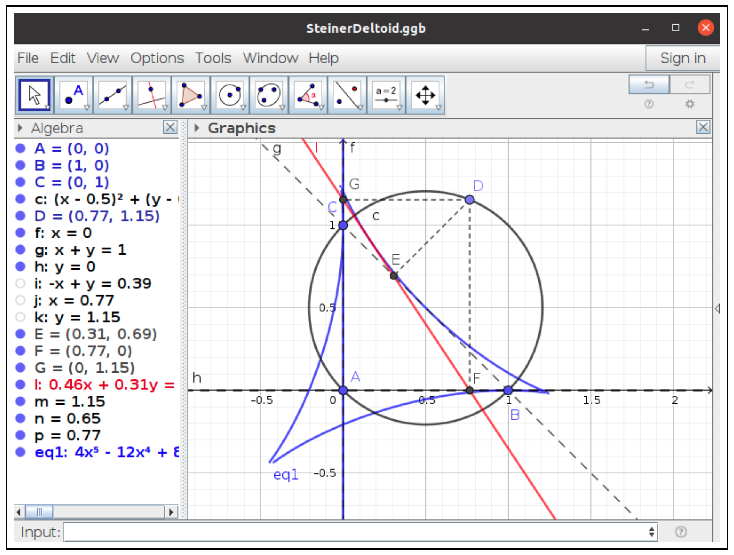
In the preceding section, we tested the Wallace–Simson theorem as a locus problem with ChatGPT, obtaining a wrong answer, and with GeoGebra, which was successful. A result derived from this theorem studies the Simson lines of a triangle, that is, the lines containing the feet of the perpendicular projections to the sides of the triangle. Considering a point moving along the circumcircle of the triangle, we can find the envelope of the family of the Simson lines. As is well known, such envelopes exist and are the hypocycloid of three cusps, called the tricuspoid curve or Steiner curve, a plane algebraic curve of a degree of four.
ChatGPT returns a correct guideline to solve the problem (see Appendix D), but does not find the envelope. Instead, it recommends using computer algebra systems or specialized software.
For its part, GeoGebra computes an envelope (Figure 6), graphs it and declares its equation to be a quintic, against the expected quartic one. Note that x is a factor, so we have x and a polynomial of a degree of four, which is the true envelope. Why does the anomalous factor x appear? The Simson line l is defined as the line passing through E end G, and, when D and C coincide, so do the feet E and G, leaving the Simson line undefined. Despite the sophisticated algebraic geometry algorithms included in GeoGebra, it does not include the one described in [22], which is the only one that could distinguish between the two factors, thus allowing for the dropping of factor x.
Table 2 summarizes the behavior of both systems with the two proposed envelopes. Despite the fact that GeoGebra deltoid results include the right answer, we give a × mark since there is a non-trivial extra factor in the equation and, regarding the plot, there is an infinite number of spurious points in the graphic object, the y-axis in Figure 6.
4. Conclusions
We tested, through some selected (but relevant, i.e., appearing in different research contexts and references) examples of plane geometric loci and families of plane curves, the abilities of ChatGPT when dealing with the computation of such loci or envelopes. Except in some simple cases, we showed that the chatbot is, at best, plausible, but not reliable. Either due to its making arithmetic errors, or by simply sketching a general guideline for solving the task, we cannot currently delegate ChatGPT for automating the search for loci. We also compared the ChatGPT results with those of GeoGebra, showing that the latter clearly surpasses the former for this particular task. However, we have also exhibited some cases showing that neither system is fully reliable.
Although it might seem that this statement is too audacious, given the small number of test cases we have analyzed, the failures we have observed are not due to unexpected errors or bugs in the design of these systems, but due to the inherent limitations in their algorithmic conception in addressing some subtle issues related to loci computations, such as, for instance, not being programmed to address, with mathematical formalism, the computation of loci or to output loci that are constructible (and not algebraic) sets. The required additional work will consist of training LLMs refined in this topic, while incorporating more powerful algorithms from algebraic geometry into GeoGebra. Until now, only specialized human knowledge has seemed capable of solving general problems in this field, with a reasonable success rate.
But this disappointing panorama can be also a source of interesting learning situations. As we hope to have clearly exemplified in the previous sections of this study, the analysis of ChatGPT’s answers and a comparison with those of GeoGebra Discovery in addressing a similar task, requires a deep and precise understanding of the basic geometry (locus, envelopes), computer algebra (e.g., Gröbner basis) and algebraic geometry (e.g., the inclusion of degeneracies, constructible sets) concepts and tools that are involved in each of the problems. And this understanding is predicated upon a previously untraveled path, as well as a non-guided exploration of the surprising, and often contradictory, outputs, whether contradictory or surprising when comparing ChatGPT and GeoGebra Discover results, or with respect to the expectations of human intuition. In summary, we think that the dialog between ChatGPT and GeoGebra Discovery can provide a rich context for developing diverse kinds of mathematical skills: problem solving, creativity, geometry, algebra, etc.
Yet, as a final remark, in connection with the title of this paper, Caveat emptor!, we would like to insist that, currently, using ChatGPT as a help for teaching situations, or even for doing mathematical research, could be valuable, but always under guidance and with caution. We reformulate the above-mentioned White–Box/Black–Box Principle for using AI chatbots in finding loci/envelopes as follows: users (students or researchers) should be aware that any results are to be taken with skepticism.
Author Contributions
All authors have participated equally in all stages of manuscript preparation. All authors have read and agreed to the published version of the manuscript.
Funding
The second author is partially supported by a “Mathematical Visualization: Foundations, Algorithms and Applications” grant (PID2020-113192GB-I00) from the Spanish MICINN.
Data Availability Statement
Data are contained in this article.
Acknowledgments
The authors would like to thank the editor and anonymous reviewers for their constructive comments and valuable suggestions that significantly improved the quality of this paper.
Conflicts of Interest
The authors declare no conflicts of interest.
Appendix A. The Wallace–Simson Theorem
- Question Consider a triangle , and a point P. Trace the orthogonal projections from P to the sides of the triangle. Find the locus of point P such that the feet of the orthogonal projections are collinear.
- ChatGPT To find the locus of point P, such that the feet of the orthogonal projections are collinear, let us consider the orthogonal projections of P onto the sides of the triangle .
Let be any point in the plane. The coordinates of the feet of the perpendiculars from P to the sides of the triangle are as follows:
- Projection onto (the line segment connecting A and B):The equation of line AB is . The foot of the perpendicular from P to will have coordinates .
- Projection onto (the line segment connecting B and C):The equation of line is . The foot of the perpendicular from P to will have coordinates .
- Projection onto (the line segment connecting A and C):The equation of line is . The foot of the perpendicular from P to will have coordinates .
Now, to ensure that the feet of the orthogonal projections are collinear, we can use the fact that the determinant of the matrix formed by these coordinates should be zero.
So, the determinant of the matrix formed by these coordinates should be zero:
Now, let us calculate this determinant:
Solving this equation will give the locus of point P, such that the feet of the orthogonal projections are collinear. Let us simplify this:
Combine like terms:
Multiply both sides by 2 to get rid of the fraction:
Combine like terms again:
This is the equation of the locus of point P, such that the feet of the orthogonal projections are collinear.
- Question Give a procedural description in GeoGebra of the above construction.
- ChatGPT Certainly! To create the construction in GeoGebra, follow these steps:
- Open GeoGebra: Open GeoGebra on your device or use the online version at www.geogebra.org.
- Create Points: Define the points for vertices A, B, and C:Click on the “Point” tool and create points , , and .
- Define Point P: Click on the “Point” tool again and create a point P with coordinates . You can use the “Input” bar to set the coordinates.
- Create Projections:To represent the projection onto (the x-axis): Click on the “Perpendicular Line” tool. Select point P and line . This creates a perpendicular line from P to .For the projection onto (vertical line at ): Click on the “Perpendicular Line” tool again. Select point P and line .For the projection onto (line ): Click on the “Perpendicular Line” tool once more. Select point P and line .
- Intersect Perpendicular Lines: Create the intersection points between the perpendicular lines and the corresponding sides of the triangle.
- Collinearity Check: Create a line through the three intersection points to check for collinearity.
- Locus Calculation: You can use the “Input” bar or the “Algebra” view to define the locus equation. For the given construction, it is .
- Animate Point P (Optional): To see how the locus changes as P moves, you can use the “Slider” tool or the “Animate” command to vary the coordinates of point P.
- Explore and Analyze: Manipulate the position of point P and observe how the feet of the orthogonal projections move and whether they remain collinear.
By following these steps, you can create an interactive GeoGebra construction that visually demonstrates the locus of points, satisfying the collinearity condition for the feet of the orthogonal projections.
Appendix B. Sketchpad Locus
- Question Let and be three fixed points. Let a be the line passing through A and . Let b be the line passing through B and . Let c be the circle with center C and radius 5. Consider a moving point G on the circle c. The line intersects line a in a point I, and line b in a point H. Find the locus of the intersection point J of lines and .
- ChatGPT To find the locus of the intersection point J of lines and , let us first find the equations of lines and c. Then, we can find the equations of lines and in terms of the parameters of the moving point G on circle c. Afterward, we can find the equation of the locus of J.
1. Equation of line a:
The line passing through points and can be represented as , where m is the slope and c is the y-intercept.
The slope, m, can be found as
Now, we have the equation of line a:
To find the value of c, plug in the coordinates of point :
So, the equation of line a is
1. Equation of line b:
The line passing through points and can be represented as follows:
The slope, m, can be found as
Now, we have the equation of line b:
To find the value of c, plug in the coordinates of point :
So, the equation of line b is
1. Equation of circle c:
The circle with center and radius 5 can be represented as follows:
Now, let us find the equations of lines and in terms of the parameter , which represents the angle that makes with the positive x-axis as G moves along circle c.
1. Equation of line :
Line passes through points and H, where H is the intersection of line b and line . The equation of line is given by
Now, we need to express m in terms of . The slope m is equal to the tangent of the angle . Since passes through the center of circle c, we can write
So, the equation of line becomes
1. Equation of line :
Line passes through points and I, where I is the intersection of line a and line . The equation of line is given by
We already know the equation of line
So, the equation of line becomes
Now, we need to express m in terms of , similar to the previous case:
So, the equation of line becomes
1. Intersection point J:
Now, we need to find the intersection point J of lines and . To do that, we can set the equations for and equal to each other and solve for x and y:
This equation simplifies to
This equation has no solution for x, which means there is no single intersection point J as G moves along circle c. In other words, the locus of J is empty or undefined.
The reason for this is that lines and are parallel to each other and will never intersect, regardless of the position of point G on circle c. Therefore, the locus of point J does not exist in this scenario.
- Question Give a procedural description suitable for GeoGebra input bar of the construction.
- ChatGPT Sure! Here is a procedural description suitable for GeoGebra’s input bar for constructing the locus of the intersection point J of lines and :
- Define the fixed points , and .
- Define the moving point G on the circle c with center and radius 5:, where t is a parameter.
- Define the coordinates of point .
- Define the coordinates of point .
- Define the equation of line a passing through points A and E:
- Define the equation of line b passing through points B and D:
- Find the intersection point I of line a and :, where satisfies the equation of circle c.
- Find the intersection point H of line b and :, where satisfies the equation of circle c.
- Define the equation of line AH passing through points A and H:
- Define the equation of line passing through points B and I:
- Find the intersection point J of lines and :, where satisfies the system of equations formed by and .
- Locus: Move the parameter t and observe the locus of point J as G moves along the circle c.
Note: Use GeoGebra’s input bar to input these commands and visualize the construction.
Please note that this description assumes you are familiar with GeoGebra’s syntax and the input bar for defining points, lines and performing geometric constructions. You may need to adapt the commands based on GeoGebra’s specific syntax and conventions.
Appendix C. The Envelope of Kissing Circles
- Question Compute the envelope of the family of circles with radius 1 centered at a point lying on the circle centered at A(0,0) and radius 1.
- ChatGPT The family of circles with radius 1 centered at points lying on the circle centered at and radius 1 forms a special case known as a “kissing circle" configuration. In this case, each circle is at a tangent to the central circle at a point on its circumference.
Let us denote the central circle as with center and radius 1. Any circle in the family can be represented by a point P on the circumference of . The center of the corresponding circle will be the point P, and its radius will be 1.
Now, let us find the envelope of this family, which is the curve formed by the points of tangency between the circles in the family and the central circle.
Consider a point P on the circumference of . The line passing through the center and the point P is a radius of . The tangent to at point P is perpendicular to this radius. Therefore, the tangent line at P has a slope equal to the negative reciprocal of the slope of the radius.
The slope of the radius (where P is on the unit circle) is given by the slope formula:
Since A is at the origin , this simplifies to .
The slope of the tangent line at P is the negative reciprocal of . Therefore, the slope of the tangent line at P is .
The equation of the tangent line passing through P is then given by the point-slope form:
Substitute :
Now, this line is the tangent to the circle centered at P with radius 1. The envelope is formed by the locus of points of tangency. To find the envelope, we need to eliminate the parameter P.
Let us denote the point of tangency as . Substituting Q into the equation above gives
Simplifying, we obtain
Multiplying both sides by y to clear the fraction:
This implies that , which means the envelope is the y-axis.
Therefore, the envelope of the family of circles with radius 1 centered at points lying on the circle centered at and radius 1 is the y-axis.
Appendix D. The Deltoid of Steiner
- Question Consider a triangle with vertices and . Let D be a point on the circumcircle of the triangle. Compute the envelope of the Simson lines when D moves along its path.
- ChatGPT The Simson line associated with a point D on the circumcircle of a triangle is a line that intersects the sides of the triangle at three points, one on each side. The envelope of Simson lines for all possible positions of D is known as the Simson–Wallace or Simson Envelope.
Given the triangle with vertices and ), let us find the equation of the circumcircle. The circumcircle of a triangle with vertices , and has the following equation:
In our case, the circumcircle equation is
Simplifying, we obtain .
Now, let D be a point on this circumcircle, so its coordinates satisfy the circumcircle equation. Let D have coordinates .
Now, for a given D, the Simson line associated with D is formed by the feet of the perpendiculars from D to the sides of the triangle. The equations of the sides of the triangle are:
- Line :
- Line :
- Line :
For a point on the circumcircle, the equations of the Simson lines can be obtained by finding the feet of perpendiculars from D to these lines.
For example, for line , the foot of the perpendicular from D is . Similarly, for line , the foot is the intersection of the perpendicular from D and line . You can find the equation of the perpendicular from D and solve it with the equation of to find the foot.
Now, the envelope of the Simson lines is the locus of the feet of these perpendiculars as D moves along its path on the circumcircle. This locus can be determined by eliminating and from the equations of the feet of the perpendiculars.
The resulting equation will describe the envelope of the Simson lines as D moves along its path on the circumcircle. Unfortunately, deriving the exact equation can be complex and may involve symbolic manipulation. You may need to use a computer algebra system for detailed calculations.
References
- Radford, A.; Narasimhan, K.; Salimans, T.; Sutskever, I. Language Models are Unsupervised Multitask Learners. OpenAI. 2019. Available online: https://cdn.openai.com/better-language-models/language_models_are_unsupervised_multitask_learners.pdf (accessed on 6 December 2023).
- ChatGPT: Optimizing Language Models for Dialogue. Available online: https://openai.com/blog/chatgpt/ (accessed on 6 December 2023).
- Huh, J.; Nelson, M.R.; Russell, C.A. ChatGPT, AI advertising, and advertising research and education. J. Advert. 2023, 52, 477–482. [Google Scholar] [CrossRef]
- Adiguzel, T.; Kaya, M.H.; Cansu, F.K. Revolutionizing education with AI: Exploring the transformative potential of ChatGPT. Contemp. Educ. Technol. 2023, 15, ep429. [Google Scholar] [CrossRef]
- Choi, J.H.; Hickman, K.E.; Monahan, A.B.; Schwarcz, D. Chatgpt goes to law school. J. Leg. Educ. 2022, 71, 387–400. [Google Scholar] [CrossRef]
- Li, J.; Dada, A.; Puladi, B.; Kleesiek, J.; Egger, J. ChatGPT in healthcare: A taxonomy and systematic review. Comput. Methods Programs Biomed. 2024, in press. [Google Scholar] [CrossRef] [PubMed]
- Sallam, M. ChatGPT utility in healthcare education, research, and practice: Systematic review on the promising perspectives and valid concerns. Healthcare 2023, 11, 887. [Google Scholar] [CrossRef] [PubMed]
- Leon, A.J.; Vidhani, D. ChatGPT needs a chemistry tutor too. J. Chem. Educ. 2023, 100, 3859–3865. [Google Scholar] [CrossRef]
- Liang, Y.; Zou, D.; Xie, H.; Wang, F.L. Exploring the potential of using ChatGPT in physics education. Smart Learn. Environ. 2023, 10, 52. [Google Scholar] [CrossRef]
- Financial Times. AI Breakthrough ChatGPT Raises Alarm over Student Cheating. 2023. Available online: https://www.ft.com/content/2e97b7ce-8223-431e-a61d-1e462b6893c3 (accessed on 6 December 2023).
- Wired. ChatGPT Is Making Universities Rethink Plagiarism. 2023. Available online: https://www.wired.com/story/chatgpt-college-university-plagiarism (accessed on 6 December 2023).
- Frieder, S.; Pinchetti, L.; Griffiths, R.; Salvatori, T.; Lukasiewicz, T.; Petersen, C.; Chevalier, A.; Berner, J. Mathematical Capabilities of ChatGPT. 2023. Available online: https://arxiv.org/pdf/2301.13867.pdf (accessed on 6 December 2023).
- Shakarian, P.; Koyyalamudi, A.; Ngu, N.; Mareedu, L. An Independent Evaluation of ChatGPT on Mathematical Word Problems (MWP). 2023. Available online: https://arxiv.org/pdf/2302.13814.pdf (accessed on 6 December 2023).
- Borji, A. A Categorical Archive of ChatGPT Failures. 2023. Available online: https://arxiv.org/pdf/2302.03494.pdf (accessed on 6 December 2023).
- Chomsky, N.; Roberts, I.; Watumull, J. The False Promise of ChatGPT. 2023. Available online: https://www.nytimes.com/2023/03/08/opinion/noam-chomsky-chatgpt-ai.html (accessed on 6 December 2023).
- Wolfram, S. Wolfram|Alpha as the Way to Bring Computational Knowledge Superpowers to ChatGPT. 2023. Available online: https://writings.stephenwolfram.com/2023/01/wolframalpha-as-the-way-to-bring-computational-knowledge-superpowers-to-chatgpt (accessed on 6 December 2023).
- Joyner, D.; Stein, W. Open Source Mathematical Software. Not. AMS 2007, 54, 1279. [Google Scholar]
- Lo, C.K. What is the impact of ChatGPT on education? A rapid review of the literature. Educ. Sci. 2023, 13, 410. [Google Scholar] [CrossRef]
- Wardat, Y.; Tashtoush, M.A.; AlAli, R.; Jarrah, A.M. ChatGPT: A revolutionary tool for teaching and learning mathematics. Eurasia J. Math. Sci. Technol. Educ. 2023, 19, em2286. [Google Scholar] [CrossRef]
- Buchberger, B. Should students learn integration rules? ACM Sigsam Bull. 1990, 24, 10–17. [Google Scholar] [CrossRef]
- Mitic, P.; Thomas, P.G. Pitfalls and limitations of computer algebra. Comput. Educ. 1994, 22, 355–361. [Google Scholar] [CrossRef]
- Abánades, M.Á.; Botana, F.; Montes, A.; Recio, T. An algebraic taxonomy for locus computation in dynamic geometry. Comput.-Aided Des. 2014, 56, 22–33. [Google Scholar] [CrossRef]
- Thom, R. Sur la théorie des enveloppes. J. MathéMatiques Pures Appliquées 1962, 41, 177–192. [Google Scholar]
- Bruce, J.W.; Giblin, P.J. Curves and Singularities: A Geometrical Introduction to Singularity Theory; Cambridge University Press: Cambridge, UK, 1992. [Google Scholar]
- Botana, F.; Abánades, M.A. Automatic deduction in (dynamic) geometry: Loci computation. Comput. Geom. 2014, 47, 75–89. [Google Scholar] [CrossRef]
- Botana, F.; Valcarce, J.L. A software tool for the investigation of plane loci. Math. Comput. Simul. 2003, 61, 139–152. [Google Scholar] [CrossRef]
- Jareš, J.; Pech, P. Exploring loci of points by DGS and CAS in teaching geometry. Electron. J. Math. Technol. 2013, 7, 143–154. [Google Scholar]
- Kovács, Z. Achievements and challenges in automatic locus and envelope animations in dynamic geometry. Math. Comput. Sci. 2019, 13, 131–141. [Google Scholar] [CrossRef]
- Thakur, A.; Wen, Y.; Chaudhuri, S. A language-agent approach to formal theorem-proving. arXiv 2023, arXiv:2310.04353. [Google Scholar]
- Trinh, T.H.; Wu, Y.; Quoc, V. Le, Q.V.; He, H. and Luong, T. Solving olympiad geometry without human demonstrations. Nature 2024, 625, 476–482. [Google Scholar] [CrossRef] [PubMed]
- Hohenwarter, M.; Borcherds, M.; Ancsin, G.; Bencze, B.; Blossier, M.; Delobelle, A.; Denizet, C.; Éliás, J.; Fekete, A.; Gál, L.; et al. GeoGebra 5 September 2014. Available online: http://www.geogebra.org (accessed on 6 December 2023).
- Kovács, Z.; Recio, T.; Vélez, M.P. Automated reasoning tools in GeoGebra discovery. ACM Commun. Comput. Algebra 2021, 55, 39–43. [Google Scholar] [CrossRef]
- GeoGebra Discovery. Available online: https://github.com/kovzol/geogebra/releases/tag/v5.0.641.0-2023Dec11 (accessed on 6 December 2023).
- Kovács, Z.; Brown, C. Recio, T.; Vajda, R. Computing with Tarski formulas and semi-algebraic sets in a web browser. J. Symb. Comput. 2024, 120, 102235. [Google Scholar] [CrossRef]
- Kovács, Z.; Parissse, B. Giac and GeoGebra—Improved Gröbner Basis Computations. In Computer Algebra and Polynomials. Lecture Notes in Computer Science; Gutierrez, J., Schicho, J., Weimann, M., Eds.; Springer International Publishing: Berlin/Heidelberg, Germany, 2015; Volume 8942. [Google Scholar] [CrossRef]
- Sutherland, I.E. Sketchpad: A man-machine graphical communication system. In Proceedings of the Spring Joint Computer Conference, Detroit, MI, USA, 21–26 May 1963; pp. 329–346. [Google Scholar]
- Botana, F.; Recio, T. Computing envelopes in dynamic geometry environments. Ann. Math. Artif. Intell. 2017, 80, 3–20. [Google Scholar] [CrossRef]
Figure 1.
A simple construction suggesting that the locus of D is a circle.

Figure 2.
The GeoGebra construction as suggested by ChatGPT.

Figure 3.
The Wallace–Simson theorem in GeoGebra.

Figure 4.
The Sketchpad classic locus in GeoGebra.

Figure 5.
Tracing the circle d, the envelope is suggested.

Figure 6.
The deltoid of Steiner with an extra linear factor.


Table 1.
Behavior of ChatGTP and GeoGebra with the proposed loci.
| ChatGPT | GeoGebra | |
|---|---|---|
| Example 1 | ✔ (needs user interaction) | ✔ equation, ✔ plot |
| Wallace–Simson | × | ✔ equation, ✔ plot |
| Sketchpad | × | ∼ equation, ✔ plot |
Table 2.
Behavior of ChatGTP and GeoGebra with the proposed envelopes.
| ChatGPT | GeoGebra | |
|---|---|---|
| Kissing circles | × | ✔ equation, ✔ plot |
| Steiner’s deltoid | × | × equation, × plot |
Disclaimer/Publisher’s Note: The statements, opinions and data contained in all publications are solely those of the individual author(s) and contributor(s) and not of MDPI and/or the editor(s). MDPI and/or the editor(s) disclaim responsibility for any injury to people or property resulting from any ideas, methods, instructions or products referred to in the content. |
© 2024 by the authors. Licensee MDPI, Basel, Switzerland. This article is an open access article distributed under the terms and conditions of the Creative Commons Attribution (CC BY) license (https://creativecommons.org/licenses/by/4.0/).
Share and Cite
MDPI and ACS Style
Botana, F.; Recio, T. Geometric Loci and ChatGPT: Caveat Emptor! Computation 2024, 12, 30. https://doi.org/10.3390/computation12020030
AMA Style
Botana F, Recio T. Geometric Loci and ChatGPT: Caveat Emptor! Computation. 2024; 12(2):30. https://doi.org/10.3390/computation12020030
Chicago/Turabian StyleBotana, Francisco, and Tomas Recio. 2024. "Geometric Loci and ChatGPT: Caveat Emptor!" Computation 12, no. 2: 30. https://doi.org/10.3390/computation12020030
Note that from the first issue of 2016, this journal uses article numbers instead of page numbers. See further details here.