
Tire–Pavement Interaction Simulation Based on Finite Element Model and Response Surface Methodology

1
Shandong High-Speed Construction Management Group Co., Ltd., Jinan 250101, China
2
School of Transportation Science and Engineering, Harbin Institute of Technology, Harbin 150090, China
*
Author to whom correspondence should be addressed.
Computation 2023, 11(9), 186; https://doi.org/10.3390/computation11090186
Submission received: 10 August 2023
/
Revised: 7 September 2023
/
Accepted: 12 September 2023
/
Published: 18 September 2023
(This article belongs to the Section Computational Engineering)
Abstract
:Acquiring accurate tire–pavement interaction information is crucial for pavement mechanical analysis and pavement maintenance. This paper combines the tire finite element model (FEM) and response surface methodology (RSM) to obtain tire–pavement interaction information and to analyze the pavement structure response under different loading conditions. A set of experiments was initially designed through the Box–Behnken design (BBD) method to obtain input and output variables for RSM calibration. The resultant RSM was evaluated accurately using the analysis of variance (ANOVA) approach. Then, tire loading simulations were conducted under different magnitudes of static loading using the optimal parameter combination obtained from the RSM. The results show that the deviations between the simulations and the real test results were mostly below 5%, validating the effectiveness of the tire FEM. Additionally, three different dynamic conditions—including free rolling, full brake, and full traction—were simulated by altering the tire rolling angle and translational velocities. Finally, the pavement mechanical response under the three rolling conditions was analyzed based on the tire–pavement contact feature.
1. Introduction
Pavement distress—such as rutting, cracking, and settlement—can jeopardize the normal use of roads. Many previous studies have been conducted to analyze the mechanical responses of pavement structures and to prolong pavement life [1,2,3]. As the primary factor contributing to pavement damage, the tire–pavement interaction has been extensively studied in previous research using test equipment. For example, the real contact stress distribution of truck tires with complex tread patterns was obtained by a test machine and was simplified into several rectangular regions, with a uniformly distributed load assumed for each region [1,4]. The contact stress distribution obtained from the dual tire was imported into a pavement structure finite element model (FEM) to analyze the shear and normal stresses at the base layer. However, due to the constraints of the test machine function, interactions under dynamic conditions—such as free rolling, traction, and braking—have rarely been examined in published research. Therefore, alternate approaches are necessary to obtain interaction details.
Simulation techniques employ a three-dimensional tire FEM to replicate the interaction between tire and pavement and to analyze the mechanical response of the pavement structure. The FEM is utilized to model the tire and to capture the resulting contact stresses on the pavement surface [5]. Based on the finite element technique, different dynamic conditions—including free rolling, full traction, full braking, and cornering—were simulated to analyze the dynamic effect on the pavement [6]. In addition, the finite element in three-dimensional loading mode was used to analytically investigate and qualify the effects of tire inclination and dynamic loading on the stress–strain responses of a pavement structure under varying loading and environmental conditions [7,8]. However, the diverse parameters of the tire have a major impact on the distribution of tire–pavement contact stress due to the complex composition of the tire structure. Thus, how to acquire the real tire parameters remains a problem. Published studies have tested the properties of tire rubber from the tread, sidewall, inner liner [9,10], and apex using the uniaxial tension test, and the elastic modulus for cords was obtained through the DMAtest. Acquiring material parameters requires many tests, which can be costly and time-consuming [11,12]. Moreover, the parameters obtained by this method cannot fully reflect the mechanical properties of rubber and cord due to the complexity of the material constitutive model [13,14]. These problems, together with inadequate accessibility to equipment, relevant test standards, and experimental conditions, have restricted the comprehensive acquisition of tire parameters through real testing. Therefore, more research studies are required to explore effective and convenient methods of deriving actual tire parameters.
The response surface methodology (RSM) is a statistical optimization technique that has recently been introduced for use in the manufacturing process [15]. This method involves fitting a mathematical expression to represent the relationship between the self-defined response and input data, and has been indicated as having good agreement with experimental data across various fields [16,17,18]. The RSM has also been applied in calibrating the bridge FEM [19,20], demonstrating its superiority in optimization. These studies concluded that the RSM can significantly increase optimization efficiency for FEMs in comparison to other optimization algorithms—such as particle swarm optimization, genetic algorithms, and grid search algorithms—that require a higher quantity of FEM computation trials during iterations.
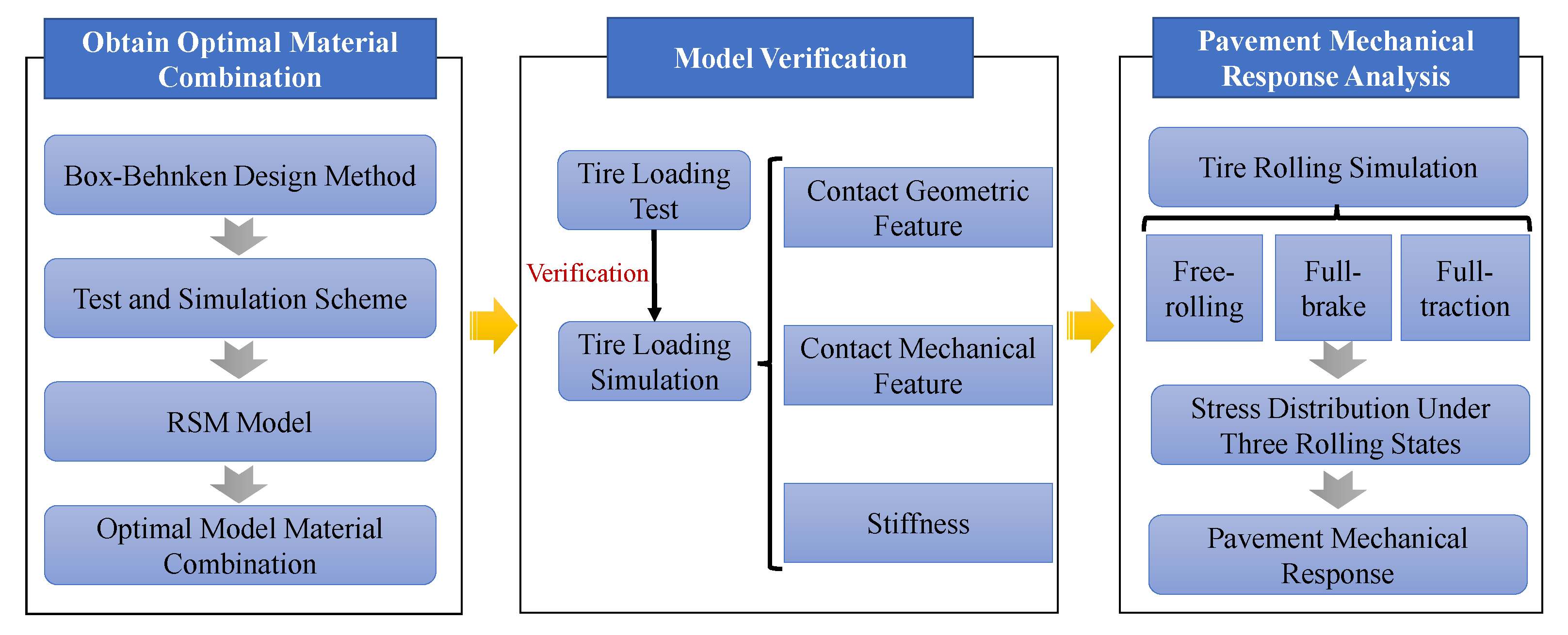
This paper combines the tire FEM and RSM to simulate the interaction between tire and pavement. The main content of this paper is outlined here. The Box–Behnken design (BBD) was initially used to create a simulation scheme with different parameter combinations that were the input variables of the RSM. Then, a static simulation was conducted according to the parameter combinations in the simulation scheme. Subsequently, a real test was conducted under the same loading condition as the simulation to determine the output data of the RSM. Following this, the RSM was established, with an analysis of variance being performed to validate the integrity of the model. An optimal parameter combination was then obtained from the RSM, and it was used in the tire finite element model. The optimal parameter combination was validated by comparing the real test results with those from the FEM under different loading conditions. After validation checking, three dynamic rolling conditions of the tire—including full traction, full braking, and free rolling—were simulated based on the FEM. In this way, the contact stress distribution at various rolling states was obtained. Finally, the stress distribution at the surface layer’s bottom was analyzed to examine the pavement’s mechanical responses under the three delineated rolling states. The framework of this paper is shown in Figure 1.
2. Calibration of the Parameter Inversion Model
This paper outlines an optimization method for tire parameters that involves several key steps. Firstly, the tire FEM is constructed and the input variables and response for the RSM are determined via simulation with a loading magnitude of 10 kN and an inflation pressure of MPa for the single tire model. Subsequently, the BBD method is implemented to create a three-level experimental scheme with four input variables. After a tire static loading simulation with different material combinations, the RSM is calibrated using the four input variables and the response, and validation is performed through analysis of variance. Finally, the optimal material combination is obtained with the RSM.
2.1. The Determination of Input Variables and Response
This paper used Abaqus to construct the tire FEM. To prepare the input variables and response for RSM, the FEM in this study employed a common type of radial tire, 12R22.5, that is preferred in transport trucks carrying heavy loads. The tire was constructed with body ply cords that run radially from bead to bead and are approximately to the center of the tread, as well as with diagonal belts that reinforce its strength and stability. Previous research has indicated that radial tires have an improved deflection capability and tread stiffness, coupled with lower rolling resistance and superior high-speed performance [21].
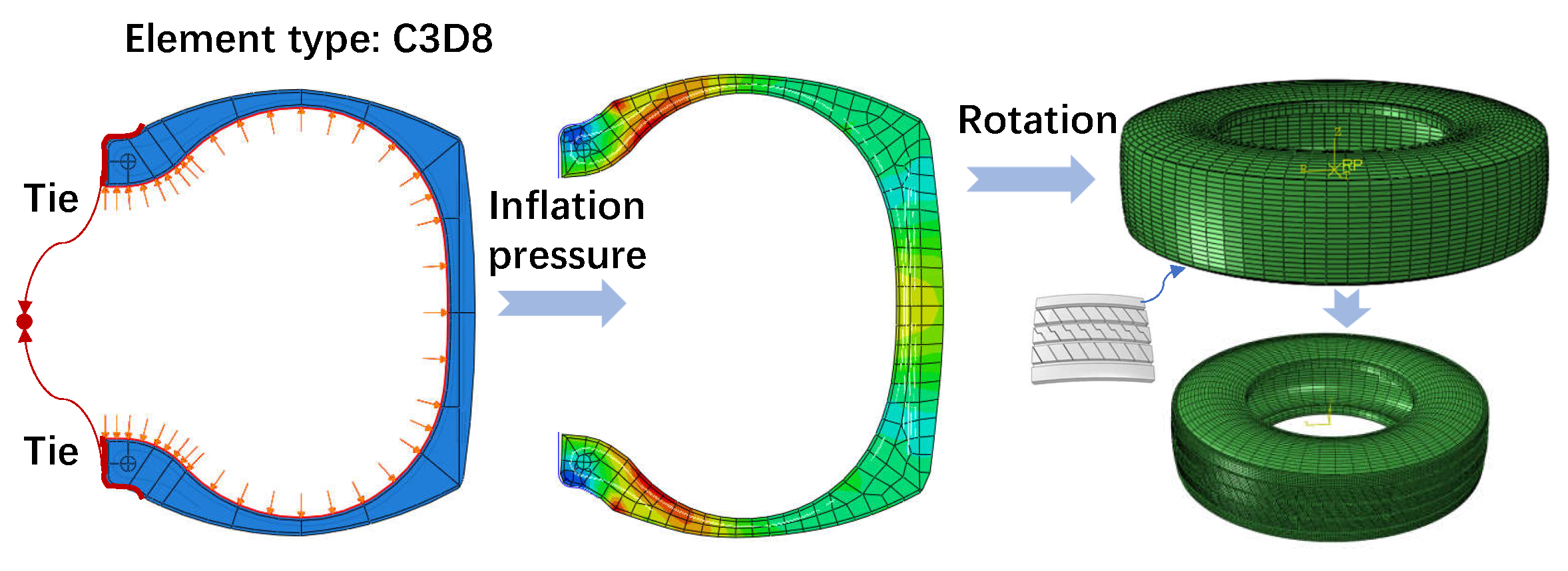
In order to construct the tire finite element model, a two-dimensional tire finite element model was first built. Then, the inflation pressure with a 0.83 MPa magnitude was exerted on the inner layer of the tire to simulate tire inflation. After that, the two-dimensional tire model was rotated in the three-dimensional model based on the simulation result. The tread was added to the tire surface by the “Tie” constraint to finish the construction of the tire finite element model. The whole procedure is shown in Figure 2.
The 12R22.5 tire is composed of rubber and a cord–rubber composite material, with rubber being nearly incompressible and hyperelastic. Researchers in the past have employed several constitutive models for modeling the properties of rubber materials, such as the Yeoh, Mooney-Rivlin, Ogden, and Neo-Hookean models. Among these models, the Yeoh model, which can reflect the large deformation of the tire, is best suited for simulating tires carrying heavy loads. Thus, the Yeoh model is adopted for tire simulation in this paper. Equation (1) is the polynomial expression of strain power.
where N denotes the polynomial order, U denotes the strain power, J denotes the elastic volume ratio, and denote the distortion, and and denote the material parameters. Due to the incompressibility of the tire, is defined as 0.
As a complex structure, a tire is composed of tread, sidewalls, beads, ply, and belts. Since the tread has direct contact with the pavement, the rubber of this structure is considered to affect the tire–pavement contact feature. Ply and belts are mainly composed of rebar, which great contributes to the strength and stiffness of tires, and thus this property was analyzed in this paper. The rebar adopts the elastic model and Young’s modulus is the factor affecting its material property. Since a small value change in Young’s modulus has little effect on the tire–pavement contact feature, its geometric properties were mainly discussed in this paper. Within the geometric feature of rebar, the angle of the cord, the interval of the cord, and the area of the cord cross-section mainly impact the feature of the tire–pavement contact area. Other parameters like the elastic modulus of steel, the density, and the Poisson ratio minorly contribute to the interaction between tire and pavement. Thus, , the angle of the cord, the interval of the cord, and the area of the cord cross-section were selected as the input variables to calibrate the RSM in this paper. In addition, the length of contact, the width of contact, and the maximum contact stress were used to represent the tire-pavement contact feature. To simplify the difficulty in calibrating the RSM, the sum of the squared errors of the three indexes above from the simulation and real test was determined as the response for the RSM.
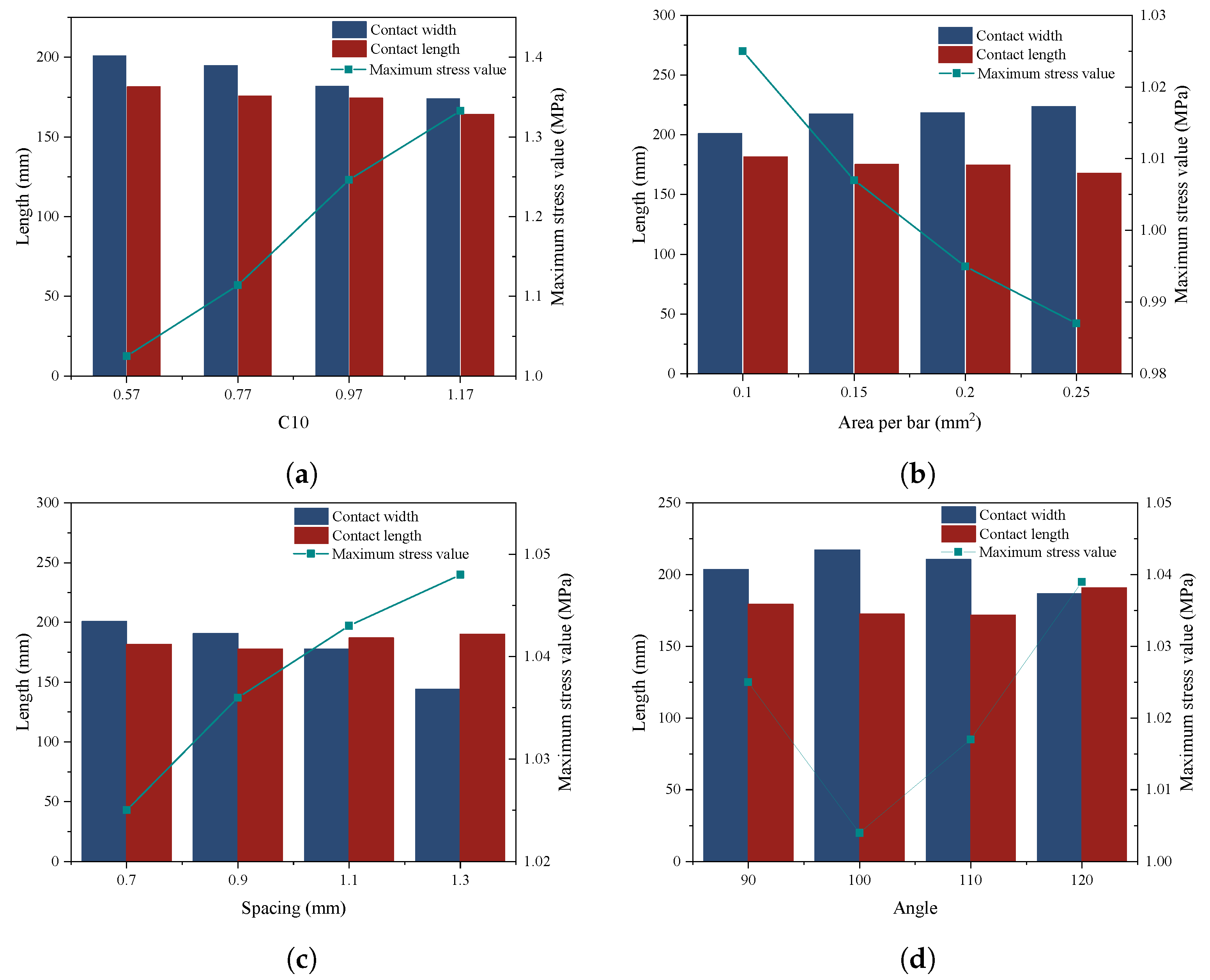
To determine the range of input variables, single-factor experiments were conducted for the four parameters, and the results are shown in Figure 3. The single-factor experiments were conducted based on the tire FEM, within which the C3D8 element was used to mesh the tire and hard contact was used to simulate the interaction between the tire and the analytical rigid road. Considering the standard inflation pressure of tire 12R22.5 and the simplification of the simulation process, this paper adopted a 0.83 MPa inflation pressure and 10 kN loading magnitude to calibrate the parameter inversion model. The load was exerted on the single tire model. With the increase in , the interval of the cord, and the angle of the cord, the maximum stress value shows a rising trend and the effect is opposite for the area of the bar. However, the value descends as the reinforcement is distributed with a larger angle.
After a group of experiments was conducted, the value ranges of the four input variables mentioned above, including , angle of the cord, interval of the cord, and area of the cord cross-section, were 0.57∼1.17, 0.1∼0.25, 0.7∼1.3, and 90∼120.
2.2. The Design of the Experiment
Different experimental design methods have been proposed in past studies to prepare experimental schemes for calibrating the RSM. Box–Behnken design and Central Composite Design are the two most commonly used methods, according to previous studies, and the BBD method is adopted in this paper. This method is suitable for optimization experiments with 2∼5 factors and three levels. The three levels are encoded by , where 0 is the central point, and and 1 represent the low and high value, respectively. Table 1 shows the value of different design parameters at each level, where the maximum and minimum values are determined according to the parameter value in Figure 3. Based on these parameter levels, the designed experiment schemes are displayed in Table 2, and the tire FEM adopts different parameter combinations to conduct tire static loading for calibrating the RSM.
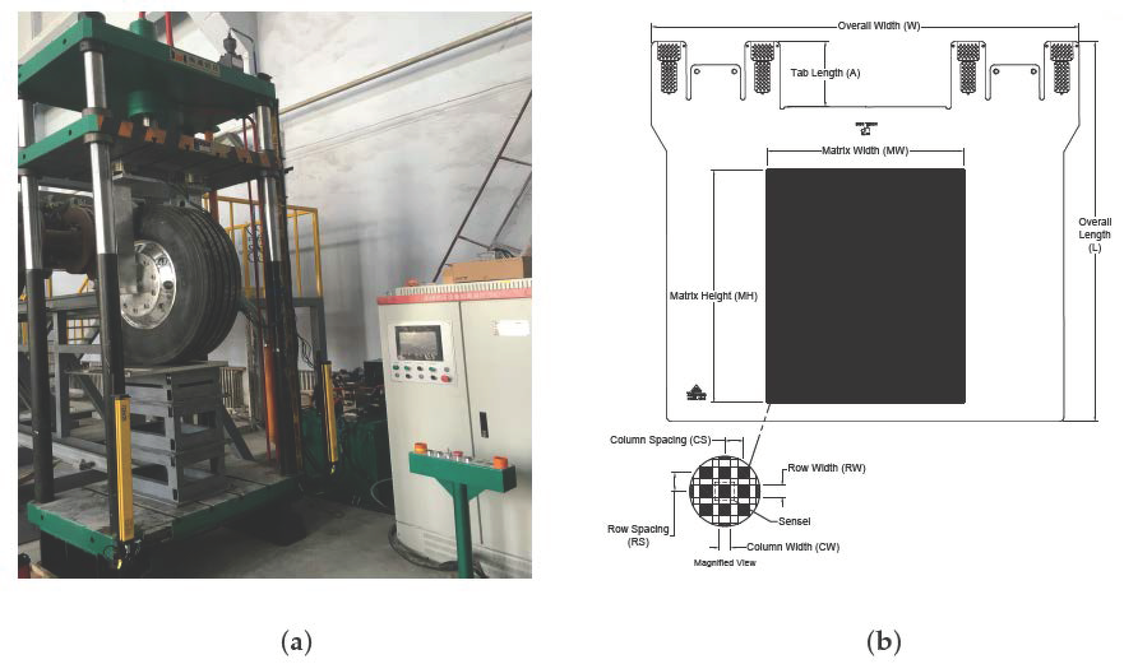
Additionally, the tire loading machine, as shown in Figure 4a, was used to conduct the tire static loading test. This machine contains position and loading magnitude sensors for monitoring the position of the tire and the loading magnitude during the process of the loading experiment. The pressure blanket, shown in Figure 4b, was placed between the tire and rigid plate to record the change in the contact feature at each frame. The result of the real test is compared with the result of the simulation in the following sections to provide the response variables for constructing the RSM.
2.3. The Calibration of the Response Surface Model
The response surface methodology is a collection of statistical and mathematical techniques used for the development of a functional relationship between inputs, denoted as , and the response y [22]. The relationship is generally unknown, but it can be approximated by a polynomial expression in the form of
where , f(x) is the function containing the powers and cross-products of powers of , is the coefficient of x and is the random error. In this paper, a second-degree polynomial model was utilized for the RSM, and the formula is expressed as
where, i represents the linear coefficient, j represents the quadratic coefficient, and k represents the number of factors included in the response surface model. In this paper, the error sum of squares for the contact width, contact length, and maximum stress value between the real test result and simulation was determined as the response.
Depending on the experimental results, the input variables and responses need normalization to avoid the impact of different units. Then, a quadratic response model can be calibrated using Equation (4). Analysis of variance is used for graphic analysis of the variance and to determine the significance of the fit polynomial model. The result is shown in Table 3. In this table, the coefficient of determination and indicate the accuracy of fit, for which a larger means better correlation. CV represents the confidence and accuracy of the experiment, and a value over 10% is preferable. is the ratio of effective signal to noise and is considered to be reasonable if it is greater than 4. The results in Table 3 show that the polynomial model satisfies the requirements of variance and significance.
where , , , and refer to the parameter, the area of the cord cross-section, the interval of the cord, and the angle of the cord, respectively.
To approximate the real tire parameters, the response was defined as 0, which means there is no error between the FEM and the real test. The obtained optimal parameter combination is shown in Table 4. The optimal parameter was then imported into the tire finite element model for validation through a tire static loading simulation.
3. The Verification of the FEM with the Optimal Parameter Combination
To verify this combination, a group of real tests were conducted using the tire loading machine at different magnitudes of loading and inflation pressure to obtain the real tire–pavement contact feature of the 12R22.5 tire on the rigid plate. The pressure blanket in Figure 4b is placed between the tire and rigid plate to record the change in the contact feature at each frame.
Simulation with a 10 kN static loading magnitude and MPa inflation pressure was conducted to obtain the contact feature of the tire. Five indexes, including contact area, footprint area, ratio of the pattern, contact length, and contact width, were used to verify the reliability of the FEM through a comparison with the real test under the same loading condition. In Table 5, it can be seen that the footprint area and the contact area of the simulation show a deviation less than from the real value. A similar result can also be seen for the contact length and width, which is within . However, the accuracy for the ratio of the pattern is rather low compared to the other indexes, especially for 25 kN, 30 kN, and kN loading magnitudes.
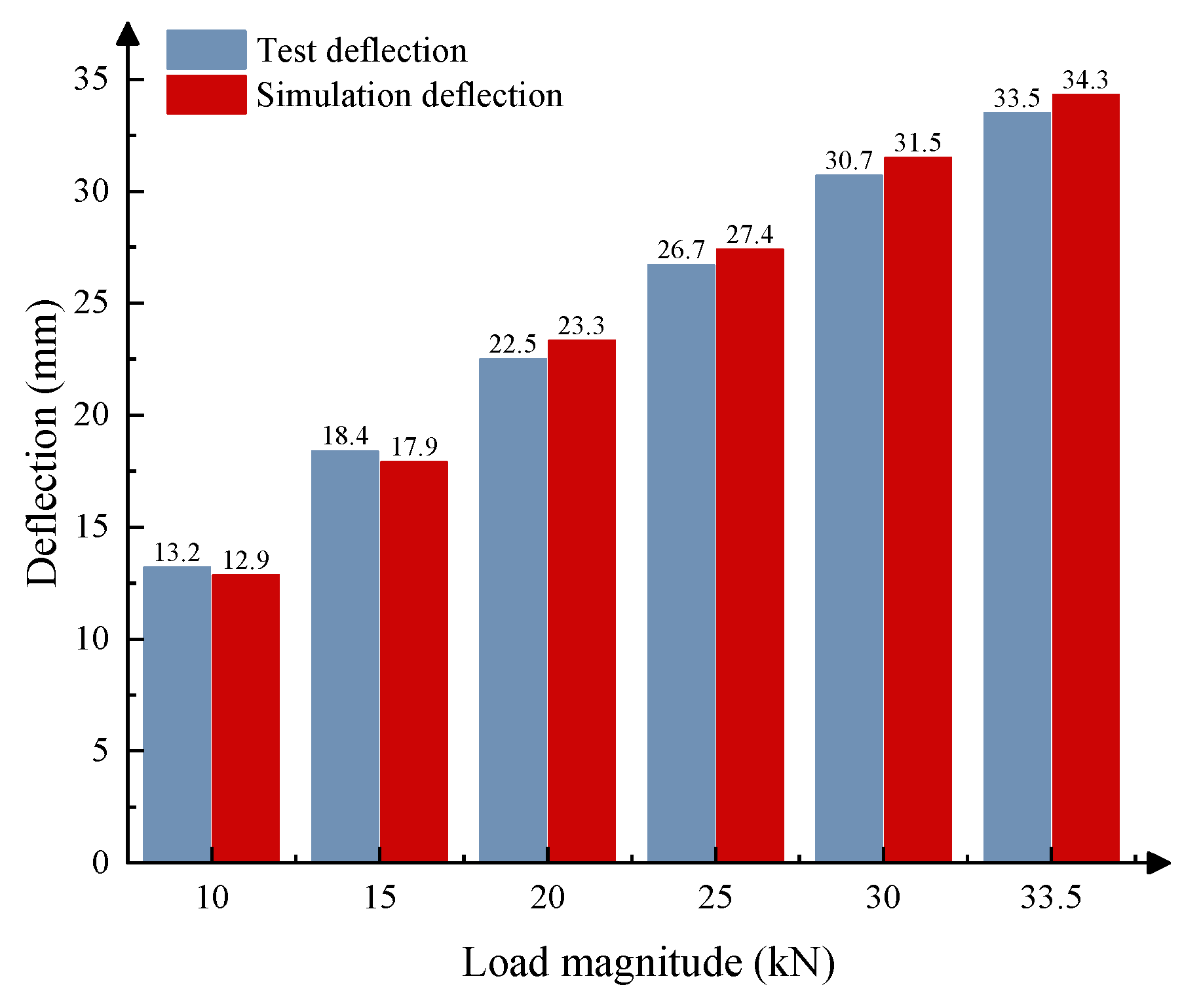
Besides the indexes verified above, the vertical deflection is another item tested in this paper to ensure the vertical stiffness of the tire is reliable. The FEM simulations with a MPa inflation pressure and a static loading magnitude ranging from 10 kN to kN were conducted and the vertical displacement of the point due to the exerted static load was recorded. Then, the result was compared with the real displacement, as shown in Figure 5. This demonstrates that the simulation displacement is larger than the true value for loading magnitudes of 10 kN and 15 kN, while the result is reversed once the loading magnitude is larger than 15 kN. In addition, the simulation is approximated to test at all conditions with only a minor difference between the two values.
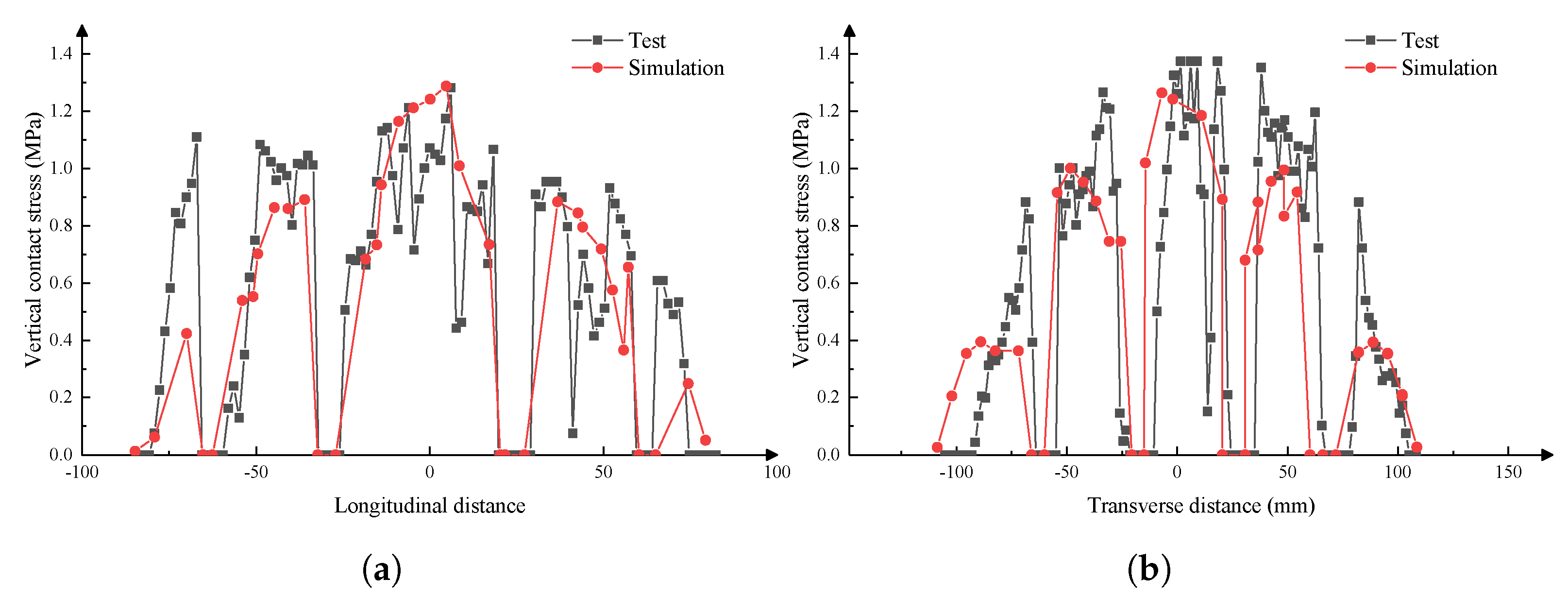
Moreover, the mechanical feature of the FEM is verified using the vertical contact stress in the central line of the longitudinal direction and transverse direction. There are several peaks and valleys, whose distribution is shown in Figure 6, where the peak refers to the tread pattern and the trench is represented by a valley. This configuration corresponds to the shape of the tire pattern. It is observed that the distribution of the vertical contact stress is similar for the simulation and test results, for which peaks and valleys are formed at the same position. However, the magnitude of the simulation is slightly lower, especially for the region away from the center of contact area. To summarize, despite some minor errors, the simulation can reasonably match the real test in both the geometric and mechanical features of the tire–pavement interaction results. This indicates that the constructed FEM is reliable in representing a real tire.
4. Tire–Pavement Interaction Simulation
4.1. The Tire Rolling Simulation
The current research has mostly investigated the interaction between the tire and road under static loading conditions using tire loading machines, while there are only a few studies that have focused on dynamic features due to the lack of equipment in this field. In this paper, three dynamic conditions including full traction, full braking, and free rolling were simulated based on the modeled three-dimensional finite element tire from the previous section by changing the angle velocity and translation velocity.
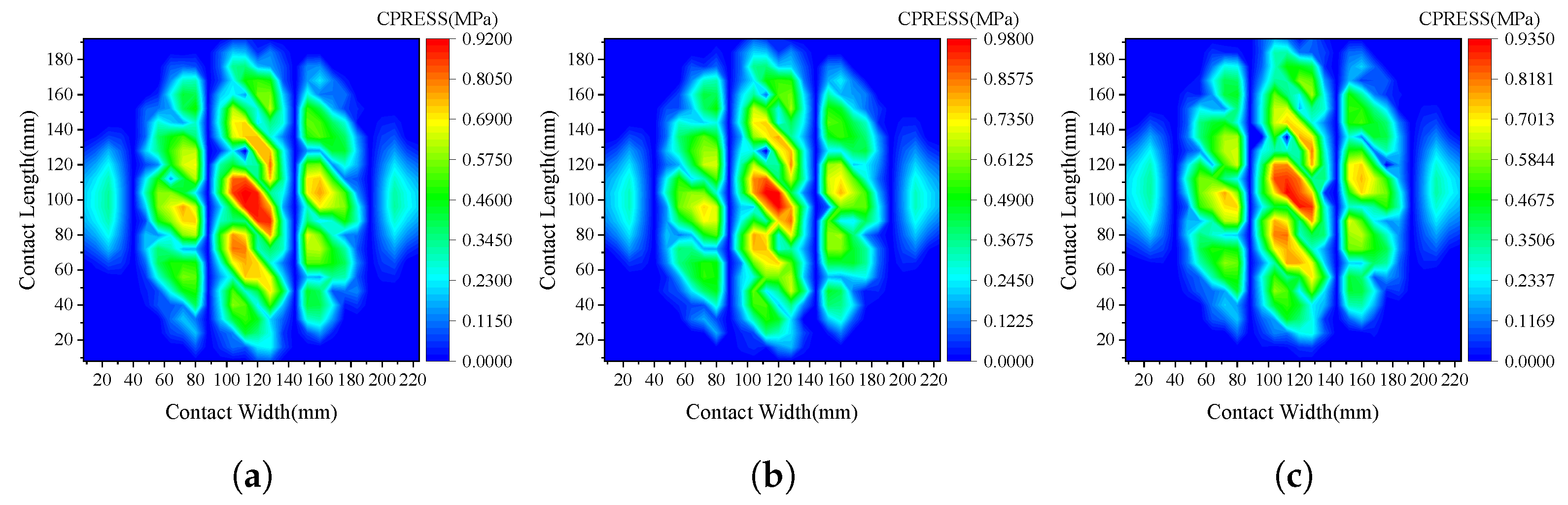
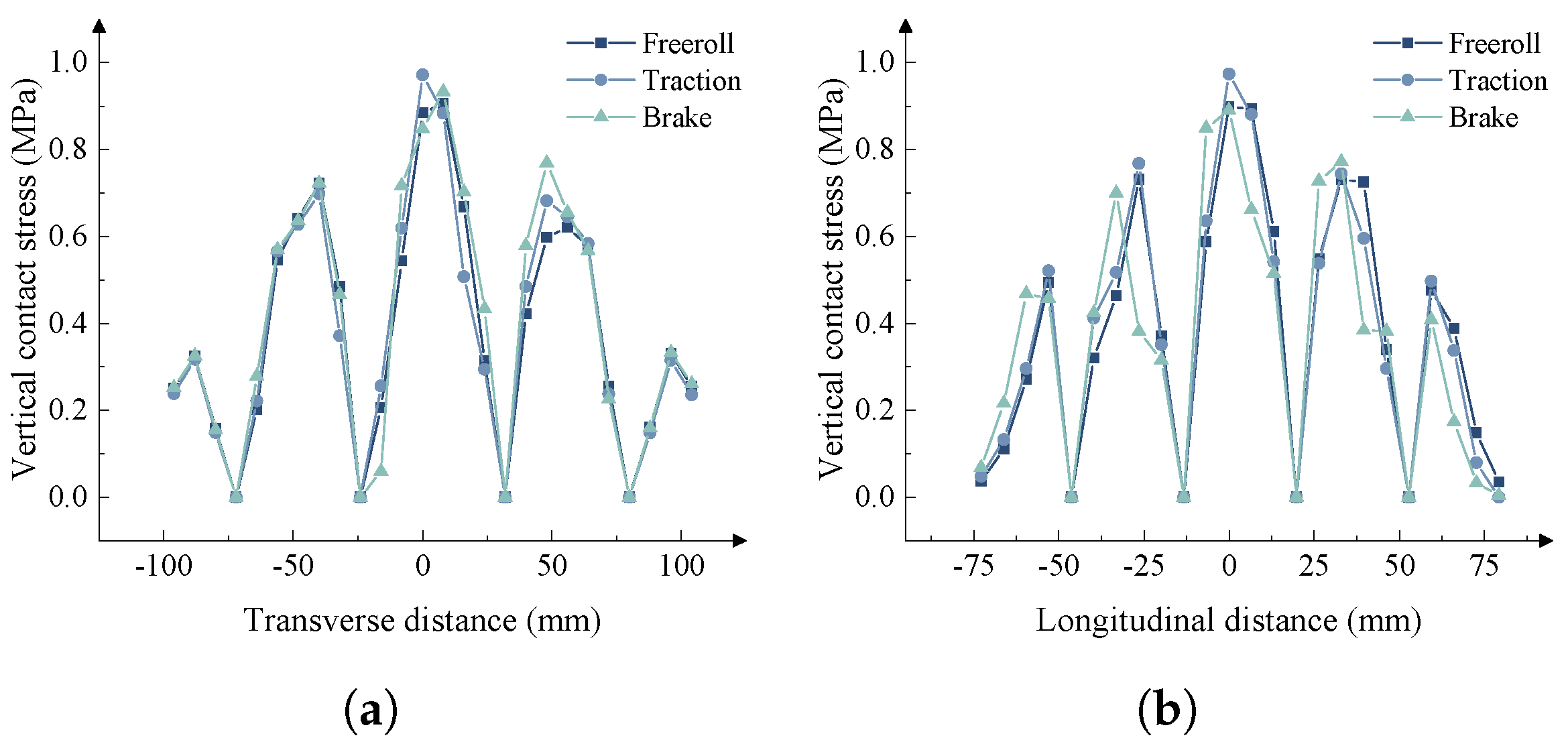
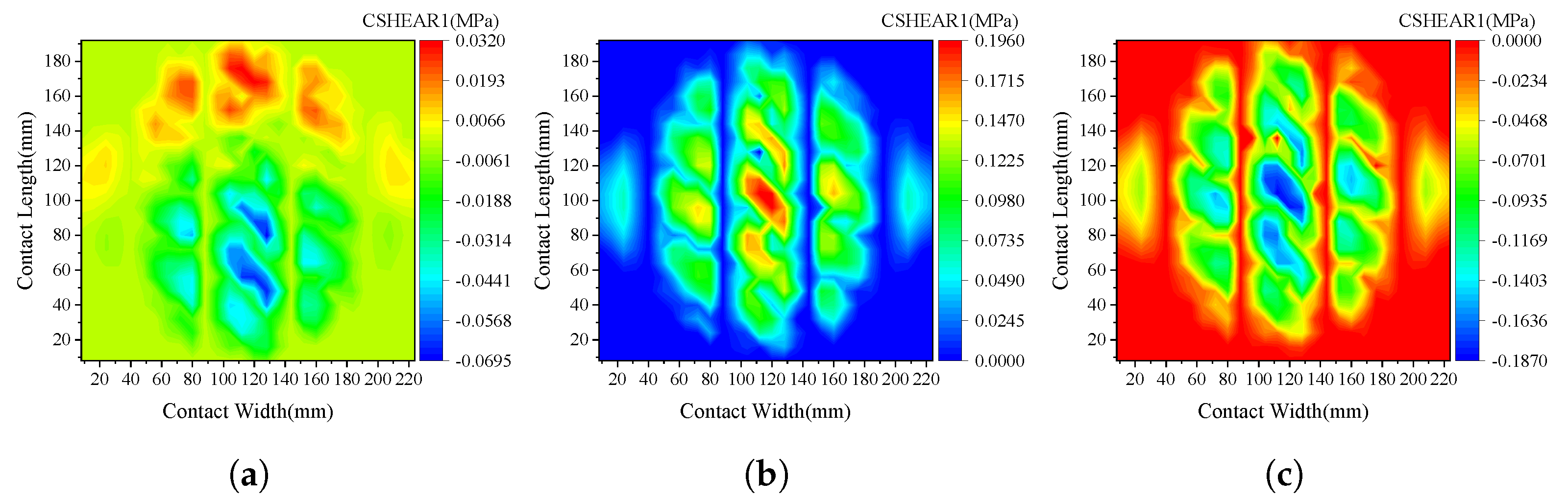
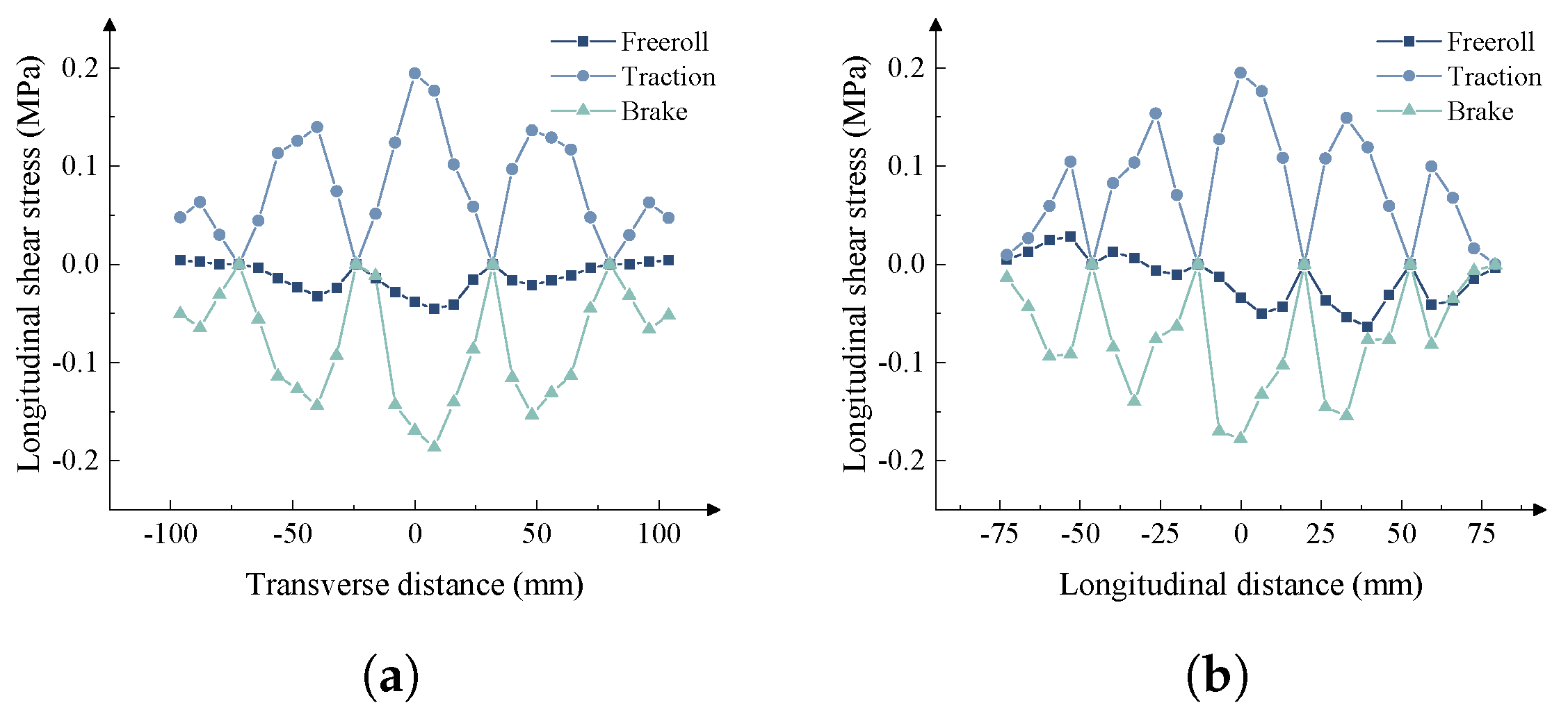
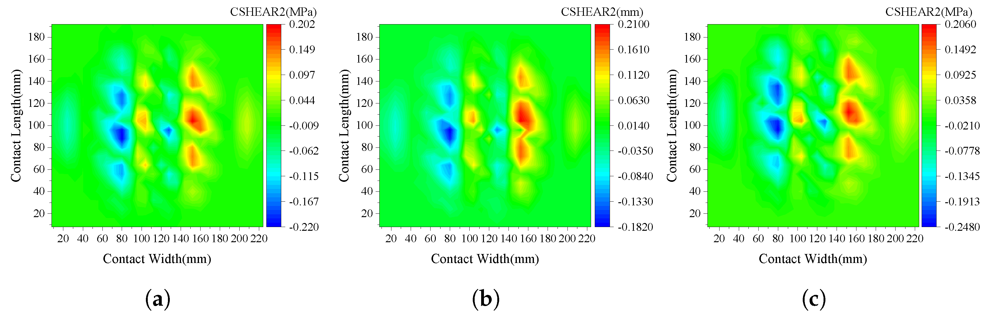
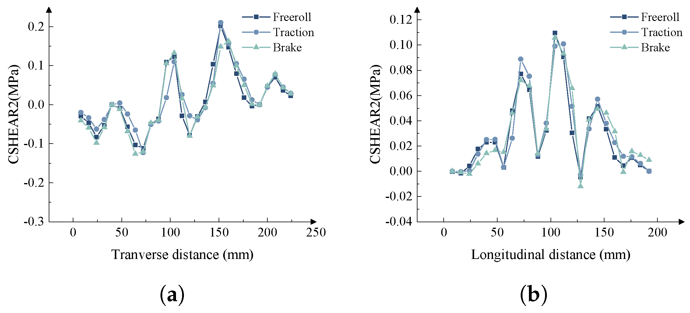
The FEM uses an angular velocity around an axis and a translation velocity in the direction of the speed to simulate different dynamic conditions of the tire. The translation speed of the tire was determined as 70 km/h and the rotation speed was set as 0 rad/s, whereas it was 36.5 rad/s to simulate the full-brake and free-roll conditions. Then, the translation speed and rotation speed were set as 0 km/h and 36.5 rad/s, respectively, to simulate the full-traction condition. The interaction between the tire and analytical road surface was defined as hard contact with a friction factor of 0.2 to simulate the friction between the tire and the road. Three indexes, including vertical contact stress, longitudinal shear stress, and transverse shear stress, were analyzed to describe the tire–pavement contact feature under dynamic conditions. For the vertical contact stress, shown in Figure 7 and Figure 8, the stress distribution for the three dynamic conditions is similar. The distribution exhibits the shape of an ellipse and the width in the transverse direction is larger than that in the longitudinal direction. It is observed that the stress magnitude decreases from the center of the contact area to the boundary. Meanwhile, the longitudinal shear stress has a different distribution in Figure 9 and Figure 10. In the traction state, the translation velocity is lower as the tire rolling speed increases, which induces the exertion of shear stress on the tire in the vehicle’s moving direction. The brake state demonstrates a reverse distribution since the translation velocity remains constant as the tire rolling speed decreases, exerting a force that pushes the tire backward. In the transition state of these two dynamic conditions, the stress in the moving direction and the opposite direction is observed at the front and back of the contact area, respectively, because the angle velocity is compatible with the translation velocity, which makes it similar to the contact feature under the static loading condition. In addition, there is little difference in the transverse stress for different states, which displays a feature of antisymmetric stress distribution along the longitudinal trench of the tread in Figure 11 and Figure 12. The tire–pavement contact distribution in this paper has similar features to the outcomes in the published literature [23,24].
As shown in Table 6, the full-traction state has more vertical contact stress and longitudinal contact stress than the free-rolling and full-brake conditions. There are minor differences for the vertical contact stress in free rolling and full braking, while their longitudinal stress demonstrates the opposite result. For the transverse contact stress, the tire-rolling states have little impact on the magnitude of stress.
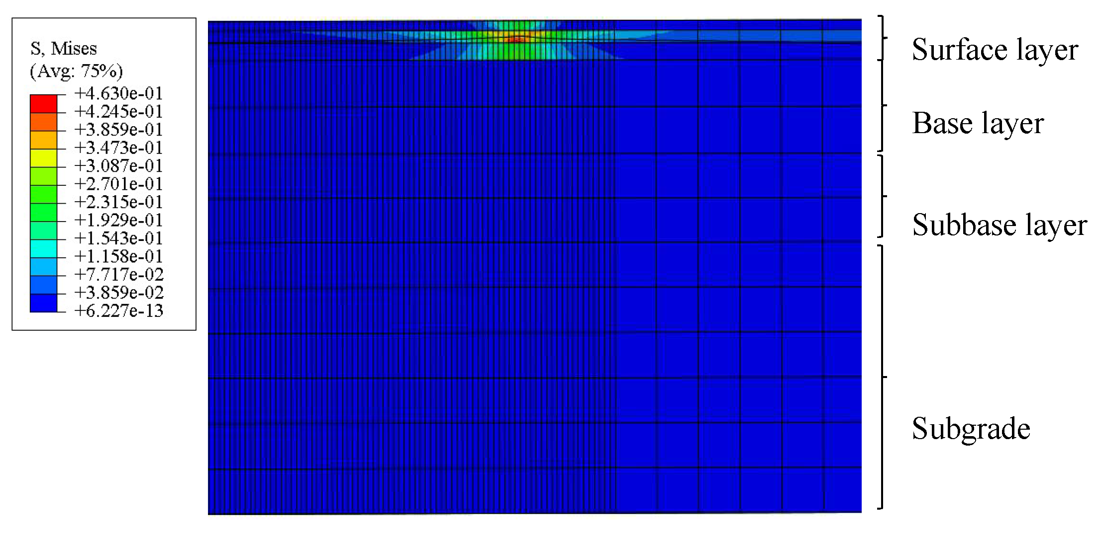
4.2. Pavement Mechanical Response Analysis
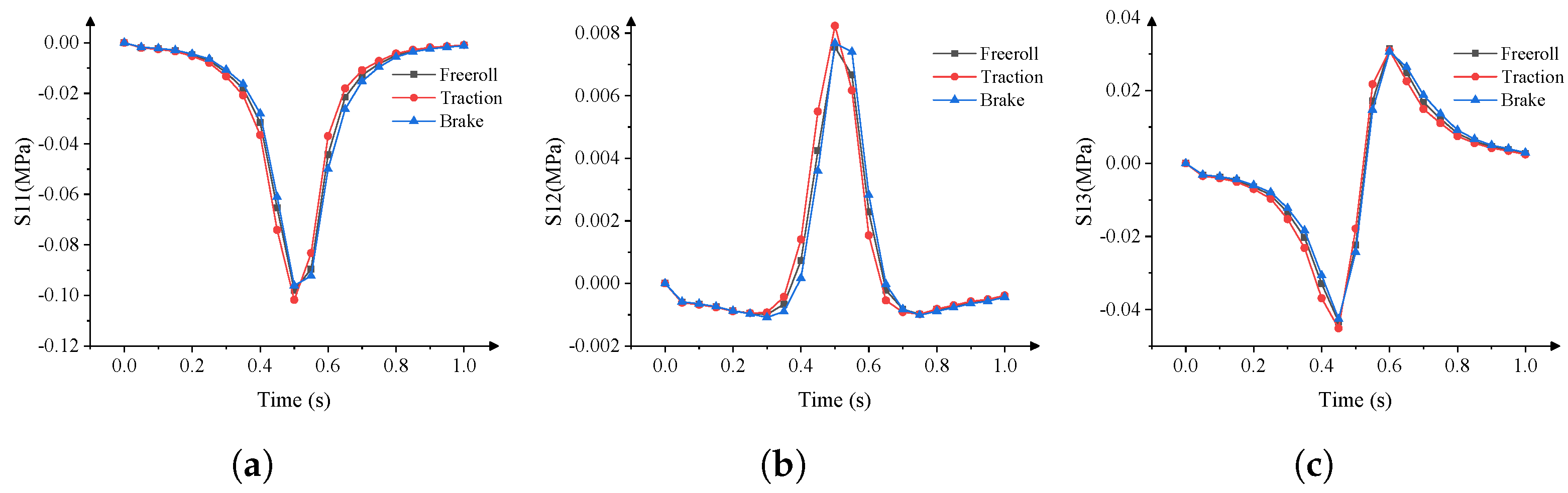
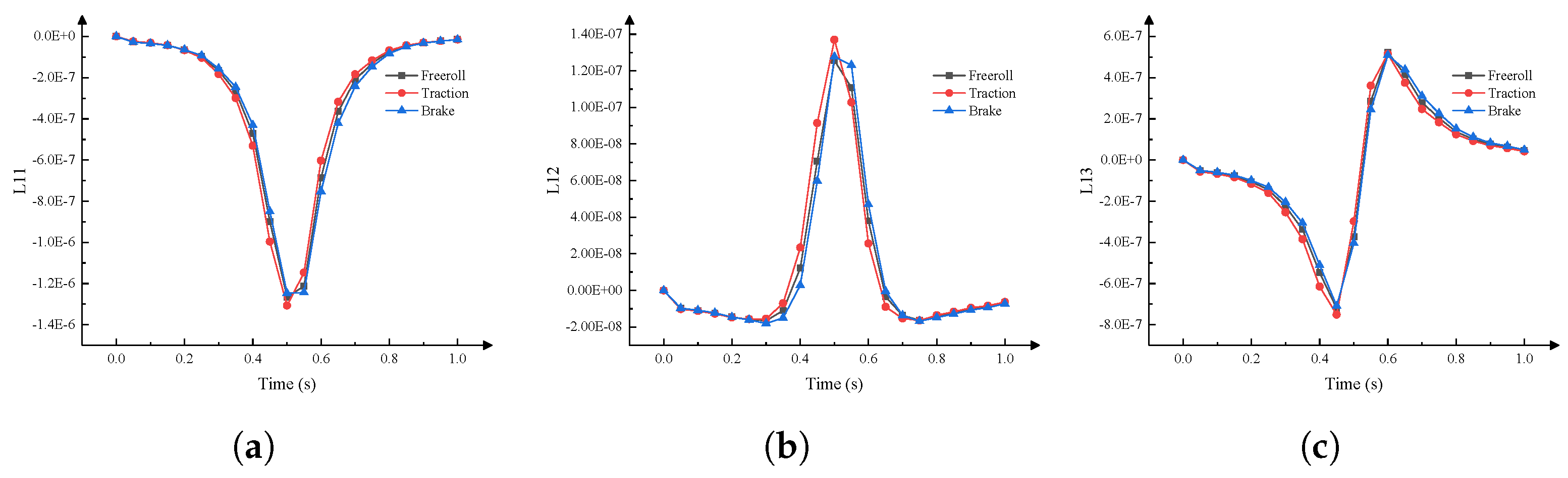
A road finite model was built to study the mechanical response of pavement to different rolling states using the property of the asphalt layer. The tire vertical contact stress and longitudinal contact stress obtained from the tire-rolling simulation were exerted on the pavement surface using a subroutine. The tire–pavement contact area was divided into several rectangular areas, within which the different magnitudes of distributed force were exerted. According to the simulation result shown in Figure 13, the mechanical response is more obvious in the surface layer rather than in other pavement structure layers. Thus, the stress at the bottom of the lower surface layer was selected to analyze the mechanical response of pavement. The change in the stress and strain with time is shown in Figure 14 and Figure 15. The line graph of S11 and S12 both show a symmetric feature with the opposite magnitude, and that for S13 is antisymmetric. Meanwhile, the pavement under traction loading initially reaches the peak of the stress magnitude earlier than that under the free-rolling state and full-brake state. The strain change feature is the same as the stress change, while there is a minor change in the strain under the tire loading. Comparing the three dynamic states, the magnitudes of stress and strain for different rolling states are close, demonstrating that the tire rolling state has little influence on the stress and strain value.
5. Conclusions
This study investigated the tire–pavement interaction and pavement mechanical response by utilizing the response surface method and tire finite element model. The RSM was calibrated using simulation and real test results following the experimental scheme created with the BBD method. Then, the optimal material combination obtained by the RSM was imported into the FEM and a tire static loading test was used to validate the effectiveness of the material parameters in the simulation. The loading test result demonstrated that the optimal material combination is suitable for the tire FEM and the parameter inversion method is reliable. Subsequently, the features of vertical, longitudinal, and transverse stress distributions under free-rolling, full-traction, and full-brake dynamic conditions were simulated by the tire FEM. The tire–pavement contact stress has different distribution features under the three rolling states. The vertical contact stress usually shows a symmetric feature and the transverse contact stress is antisymmetric along the center line of the tire surface. Additionally, the longitudinal stress is symmetric under the traction and brake conditions, while its magnitude changes from positive to negative along the rolling direction under the free-rolling state. These results are similar to the results presented in other studies. Finally, the pavement mechanical response was obtained based on the tire contact stress under the three rolling states. It was shown that the mechanical response is most obvious in the surface layer and the rolling state affects the time when the highest value of magnitude appears. The method used in this paper can be helpful in constructing tire FEMs and improving the accuracy of tire loading simulations. The tire–pavement interaction information can be acquired accurately, which supports the establishment of an interaction information dataset for different sorts of tires. Combined with deep learning methods like ContactGAN [25], the tire–pavement contact stress distribution can be quickly predicted, which will promote the development of pavement mechanical response analysis in the future.
Author Contributions
Conceptualization, X.M., Z.D. and Y.Y.; methodology, X.M., Q.Z. and T.L.; software, Q.Z., L.S. and X.M.; validation, L.S., Y.Y., Z.D. and Q.Z.; formal analysis, Z.D., L.S. and T.L.; investigation, Q.Z. and T.L.; resources, Q.Z. and X.M.; data curation, L.S.; writing—original draft preparation, Q.Z. and T.L.; writing—review and editing, L.S., X.M., Y.Y. and Z.D.; visualization, L.S.; supervision, T.L., Y.Y., Q.Z. and Z.D.; project administration, T.L. and Q.Z.; funding acquisition, Q.Z. and Y.Y. All authors have read and agreed to the published version of the manuscript.
Funding
This work was supported by the project “Early Warning and Rapid Processing Technology for Expressway Pavement Icing”.
Institutional Review Board Statement
Not applicable.
Informed Consent Statement
Not applicable.
Data Availability Statement
Not applicable.
Conflicts of Interest
The authors declare no conflict of interest.
References
- Guan, J.; Zhou, X.; Liu, L.; Ran, M. Measurement of Tire-Pavement Contact Tri-Axial Stress Distribution Based on Sensor Array. Coatings 2023, 13, 416. [Google Scholar] [CrossRef]
- Zhu, X.; Zhang, Q.; Chen, L.; Du, Z. Mechanical response of hydronic asphalt pavement under temperature–vehicle coupled load: A finite element simulation and accelerated pavement testing study. Constr. Build. Mater. 2021, 272, 121884. [Google Scholar] [CrossRef]
- Assogba, O.C.; Tan, Y.; Zhou, X.; Zhang, C.; Anato, J.N. Numerical investigation of the mechanical response of semi-rigid base asphalt pavement under traffic load and nonlinear temperature gradient effect. Constr. Build. Mater. 2020, 235, 117406. [Google Scholar] [CrossRef]
- Hu, X.; Sun, L. Stress response analysis of asphalt pavement under measured tire ground pressure of heavy vehicle. J.-Tongji Univ. 2006, 34, 64. [Google Scholar]
- Ge, H.; Quezada, J.C.; Le Houerou, V.; Chazallon, C. Multiscale analysis of tire and asphalt pavement interaction via coupling FEM–DEM simulation. Eng. Struct. 2022, 256, 113925. [Google Scholar] [CrossRef]
- Assogba, O.C.; Sun, Z.; Tan, Y.; Nonde, L.; Bin, Z. Finite-element simulation of instrumented asphalt pavement response under moving vehicular load. Int. J. Geomech. 2020, 20, 04020006. [Google Scholar] [CrossRef]
- Hu, X.; Faruk, A.N.; Zhang, J.; Souliman, M.I.; Walubita, L.F. Effects of tire inclination (turning traffic) and dynamic loading on the pavement stress–strain responses using 3-D finite element modeling. Int. J. Pavement Res. Technol. 2017, 10, 304–314. [Google Scholar] [CrossRef]
- Behnke, R.; Wollny, I.; Hartung, F.; Kaliske, M. Thermo-mechanical finite element prediction of the structural long-term response of asphalt pavements subjected to periodic traffic load: Tire-pavement interaction and rutting. Comput. Struct. 2019, 218, 9–31. [Google Scholar] [CrossRef]
- Yang, X.; Olatunbosun, O.; Bolarinwa, E. Materials testing for finite element tire model. Sae Int. J. Mater. Manuf. 2010, 3, 211–220. [Google Scholar] [CrossRef]
- Arachchi, N.; Abegunasekara, C.; Premarathna, W.; Jayasinghe, J.; Bandara, C.; Ranathunga, R. Finite Element Modeling and Simulation of Rubber Based Products: Application to Solid Resilient Tire. In Proceedings of the ICSECM 2019: Proceedings of the 10th International Conference on Structural Engineering and Construction Management; Springer: Berlin/Heidelberg, Germany, 2021; pp. 517–531. [Google Scholar]
- Boyce, M.C.; Arruda, E.M. Constitutive models of rubber elasticity: A review. Rubber Chem. Technol. 2000, 73, 504–523. [Google Scholar] [CrossRef]
- Yeoh, O.H. Some forms of the strain energy function for rubber. Rubber Chem. Technol. 1993, 66, 754–771. [Google Scholar] [CrossRef]
- Ogden, R. Nearly isochoric elastic deformations: Application to rubberlike solids. J. Mech. Phys. Solids 1978, 26, 37–57. [Google Scholar] [CrossRef]
- Meyer, K.H.; Ferri, C. The elasticity of rubber. Rubber Chem. Technol. 1935, 8, 319–334. [Google Scholar] [CrossRef]
- Giovanni, M. Response Surface Methodology and Product Optimization; Wiley: Hoboken, NJ, USA, 1983. [Google Scholar]
- Li, J.; Zuo, W.; Jiaqiang, E.; Zhang, Y.; Li, Q.; Sun, K.; Zhou, K.; Zhang, G. Multi-objective optimization of mini U-channel cold plate with SiO2 nanofluid by RSM and NSGA-II. Energy 2022, 242, 123039. [Google Scholar] [CrossRef]
- Pali, H.S.; Sharma, A.; Kumar, N.; Singh, Y. Biodiesel yield and properties optimization from Kusum oil by RSM. Fuel 2021, 291, 120218. [Google Scholar] [CrossRef]
- Benzannache, N.; Belaadi, A.; Boumaaza, M.; Bourchak, M. Improving the mechanical performance of biocomposite plaster/Washingtonian filifira fibres using the RSM method. J. Build. Eng. 2021, 33, 101840. [Google Scholar] [CrossRef]
- Yang, H.; Xu, X.; Neumann, I. Optimal finite element model with response surface methodology for concrete structures based on Terrestrial Laser Scanning technology. Compos. Struct. 2018, 183, 2–6. [Google Scholar] [CrossRef]
- Rajabi, M.; Aboutalebi, M.; Seyedein, S.; Ataie, S. Simulation of residual stress in thick thermal barrier coating (TTBC) during thermal shock: A response surface-finite element modeling. Ceram. Int. 2022, 48, 5299–5311. [Google Scholar] [CrossRef]
- Gent, A.N.; Walter, J.D. Pneumatic Tire 2006. Available online: https://ideaexchange.uakron.edu/mechanical_ideas/854 (accessed on 11 September 2023).
- Khuri, A.I.; Mukhopadhyay, S. Response surface methodology. Wiley Interdiscip. Rev. Comput. Stat. 2010, 2, 128–149. [Google Scholar] [CrossRef]
- Wang, T.; Dong, Z.; Xu, K.; Ullah, S.; Wang, D.; Li, Y. Numerical simulation of mechanical response analysis of asphalt pavement under dynamic loads with non-uniform tire-pavement contact stresses. Constr. Build. Mater. 2022, 361, 129711. [Google Scholar] [CrossRef]
- Wang, H.; Al-Qadi, I.L.; Stanciulescu, I. Simulation of tyre–pavement interaction for predicting contact stresses at static and various rolling conditions. Int. J. Pavement Eng. 2012, 13, 310–321. [Google Scholar] [CrossRef]
- Liu, X.; Jayme, A.; Al-Qadi, I.L. ContactGAN development–prediction of tire-pavement contact stresses using a generative and transfer learning model. Int. J. Pavement Eng. 2022, 1–11. [Google Scholar] [CrossRef]
Figure 1.
The framework of the paper.

Figure 2.
The procedure of constructing tire finite element model.

Figure 3.
The effect of different parameters. (a) The effect of C10. (b) The effect of area per bar. (c) The effect of spacing. (d) The effect of angle.
Figure 3.
The effect of different parameters. (a) The effect of C10. (b) The effect of area per bar. (c) The effect of spacing. (d) The effect of angle.

Figure 4.
Tire loading equipment. (a) Tire loading machine. (b) The pressure blanket.

Figure 5.
The deflection of the tire.

Figure 6.
Mechanical feature of FEM. (a) Stress distribution in longitudinal direction; (b) stress distribution in transverse direction.
Figure 6.
Mechanical feature of FEM. (a) Stress distribution in longitudinal direction; (b) stress distribution in transverse direction.

Figure 7.
Vertical contact stress. (a) Free rolling; (b) full traction; (c) full braking.

Figure 8.
The distribution of vertical contact stress. (a) Transverse distribution; (b) longitudinal distribution.
Figure 8.
The distribution of vertical contact stress. (a) Transverse distribution; (b) longitudinal distribution.

Figure 9.
Longitudinal shear stress. (a) Free rolling; (b) full traction; (c) full braking.

Figure 10.
The distribution of longitudinal shear stress. (a) Transverse distribution; (b) longitudinal distribution.
Figure 10.
The distribution of longitudinal shear stress. (a) Transverse distribution; (b) longitudinal distribution.

Figure 11.
The transverse shear stress of three dynamic conditions. (a) Free rolling; (b) full traction; (c) full braking.
Figure 11.
The transverse shear stress of three dynamic conditions. (a) Free rolling; (b) full traction; (c) full braking.

Figure 12.
The distribution of transverse shear stress. (a) Transverse distribution; (b) longitudinal distribution.
Figure 12.
The distribution of transverse shear stress. (a) Transverse distribution; (b) longitudinal distribution.

Figure 13.
Mechanical response.

Figure 14.
The stress at the bottom of the surface layer. (a) S11; (b) S12; (c) S13.

Figure 15.
The strain at the bottom of the surface layer. (a) L11; (b) L12; (c) L13.


Table 1.
The design parameter and the value at each level.
| Parameter | Level | ||
|---|---|---|---|
| −1 | 0 | 1 | |
| C10 (MPa) | 0.57 | 0.87 | 1.17 |
| Angle of cord (°) | 90 | 105 | 120 |
| Interval of cord (mm) | 0.7 | 1 | 1.3 |
| Area of cord cross-section (mm2) | 0.1 | 0.175 | 0.25 |
Table 2.
Design experiment.
| Serial Number | C10 (MPa) | Area of Cord Cross-Section (mm2) | Interval of Cord (mm) | Angle of Cord (°) |
|---|---|---|---|---|
| 1 | 1.17 | 0.25 | 1 | 105 |
| 2 | 0.87 | 0.25 | 0.7 | 105 |
| 3 | 0.87 | 0.1 | 1.3 | 105 |
| 4 | 0.57 | 0.175 | 1 | 120 |
| 5 | 1.17 | 0.1 | 1 | 105 |
| 6 | 0.87 | 0.175 | 1.3 | 90 |
| 7 | 0.57 | 0.175 | 0.7 | 105 |
| 8 | 0.87 | 0.175 | 1 | 105 |
| 9 | 0.87 | 0.25 | 1 | 120 |
| 10 | 0.57 | 0.175 | 1.3 | 105 |
| 11 | 1.17 | 0.175 | 0.7 | 105 |
| 12 | 0.57 | 0.175 | 1 | 90 |
| 13 | 0.57 | 0.25 | 1 | 105 |
| 14 | 0.87 | 0.175 | 1 | 105 |
| 15 | 0.87 | 0.175 | 1 | 105 |
| 16 | 0.87 | 0.175 | 0.7 | 120 |
| 17 | 0.87 | 0.1 | 1 | 120 |
| 18 | 0.87 | 0.175 | 0.7 | 90 |
| 19 | 0.87 | 0.1 | 0.7 | 105 |
| 20 | 0.87 | 0.25 | 1.3 | 105 |
| 21 | 1.17 | 0.175 | 1.3 | 105 |
| 22 | 0.87 | 0.1 | 1 | 90 |
| 23 | 1.17 | 0.175 | 1 | 120 |
| 24 | 0.87 | 0.175 | 1 | 105 |
| 25 | 0.57 | 0.1 | 1 | 105 |
| 26 | 0.87 | 0.175 | 1 | 105 |
| 27 | 1.17 | 0.175 | 1 | 90 |
| 28 | 0.87 | 0.175 | 1.3 | 120 |
| 29 | 0.87 | 0.25 | 1 | 90 |
Table 3.
The analysis of variance.
| Index | Std. Dev. | Adjusted | Mean | C.V. (%) | Adeq Precision | |
|---|---|---|---|---|---|---|
| Value | 0.14 | 0.91 | 0.83 | 0.75 | 19.42 | 11.85 |
Table 4.
The optimal parameter combination.
| Item | C10 (MPa) | Angle of Cord (°) | Interval of Cord (mm) | Area of Cord Cross-Section (mm2) |
|---|---|---|---|---|
| Value | 1.166 | 0.25 | 1.3 | 100 |
Table 5.
The verification of the geometry feature.
| Loading Magnitude (kN) | 10 | 15 | 20 | 25 | 30 | 33.5 | |
|---|---|---|---|---|---|---|---|
| Error rate (%) | Footprint area | 2.07 | 1.45 | 0.18 | 0.23 | 0.69 | 0.82 |
| Contact area | 2.06 | 2.30 | 0.82 | 1.52 | 2.03 | 0.17 | |
| Ratio of pattern | 0.05 | 3.72 | 2.81 | 8.39 | 6.46 | 4.80 | |
| Contact length | 3.59 | 0.33 | 0.80 | 1.11 | 3.39 | 4.22 | |
| Contact width | 0.45 | 4.30 | 1.76 | 1.76 | 1.32 | 0.43 | |
Table 6.
Comparison of different contact stresses.
| Direction | Vertical Contact Stress (MPa) | Longitudinal Contact Stress (MPa) | Transverse Contact Stress (MPa) | |
|---|---|---|---|---|
| Longitudinal | Free rolling | 0.920 | 0.052 | 0.115 |
| Full traction | 1.035 | 0.211 | 0.101 | |
| Full braking | 0.921 | 0.190 | 0.110 | |
| Transverse | Free rolling | 0.918 | 0.041 | 0.203 |
| Full traction | 1.031 | 0.214 | 0.202 | |
| Full braking | 0.929 | 0.191 | 0.202 | |
Disclaimer/Publisher’s Note: The statements, opinions and data contained in all publications are solely those of the individual author(s) and contributor(s) and not of MDPI and/or the editor(s). MDPI and/or the editor(s) disclaim responsibility for any injury to people or property resulting from any ideas, methods, instructions or products referred to in the content. |
© 2023 by the authors. Licensee MDPI, Basel, Switzerland. This article is an open access article distributed under the terms and conditions of the Creative Commons Attribution (CC BY) license (https://creativecommons.org/licenses/by/4.0/).
Share and Cite
MDPI and ACS Style
Zhang, Q.; Shangguan, L.; Li, T.; Ma, X.; Yin, Y.; Dong, Z. Tire–Pavement Interaction Simulation Based on Finite Element Model and Response Surface Methodology. Computation 2023, 11, 186. https://doi.org/10.3390/computation11090186
AMA Style
Zhang Q, Shangguan L, Li T, Ma X, Yin Y, Dong Z. Tire–Pavement Interaction Simulation Based on Finite Element Model and Response Surface Methodology. Computation. 2023; 11(9):186. https://doi.org/10.3390/computation11090186
Chicago/Turabian StyleZhang, Qingtao, Lingxiao Shangguan, Tao Li, Xianyong Ma, Yunfei Yin, and Zejiao Dong. 2023. "Tire–Pavement Interaction Simulation Based on Finite Element Model and Response Surface Methodology" Computation 11, no. 9: 186. https://doi.org/10.3390/computation11090186
Note that from the first issue of 2016, this journal uses article numbers instead of page numbers. See further details here.