
Sensitivity Analysis of Mathematical Models


Department of Applied Mathematics, Lipetsk State Technical University, Moskovskaya Str., 30, RU-398055 Lipetsk, Russia
Computation 2023, 11(8), 159; https://doi.org/10.3390/computation11080159
Submission received: 15 July 2023
/
Revised: 8 August 2023
/
Accepted: 12 August 2023
/
Published: 14 August 2023
Abstract
:The construction of a mathematical model of a complicated system is often associated with the evaluation of inputs’ (arguments, factors) influence on the output (response), the identification of important relationships between the variables used, and reduction of the model by decreasing the number of its inputs. These tasks are related to the problems of Sensitivity Analysis of mathematical models. The author proposes an alternative approach based on applying Analysis of Finite Fluctuations that uses the Lagrange mean value theorem to estimate the contribution of changes to the variables of a function to the output change. The article investigates the presented approach on an example of a class of fully connected neural network models. As a result of Sensitivity Analysis, a set of sensitivity measures for each input is obtained. For their averaging, it is proposed to use a point-and-interval estimation algorithm using Tukey’s weighted average. The comparison of the described method with the computation of Sobol’s indices is given; the consistency of the proposed method is shown. The computational robustness of the procedure for finding sensitivity measures of inputs is investigated. Numerical experiments are carried out on the neuraldat data set of the NeuralNetTools library of the R data processing language and on data of the healthcare services provided in the Lipetsk region.
1. Introduction
Being an important point in system investigation, Sensitivity Analysis (SA) is the study of how input uncertainty influences the uncertainty of outputs [1]. Depending on the purpose, a task like that could be helpful in solving the following problems: (1) to test how robust the results of a model or a system are; (2) to understand the relationships between outputs and inputs; (3) to reduce the uncertainty by choosing the most significant inputs; (4) to find errors in a model or a system by defining unexpected relationships between outputs and inputs; (5) to simplify a model by removing inputs that do not have a strong affect on outputs; (6) to make a model more interpretative by finding an understandable explanation of inputs; etc.
Depending on the tools used, many directions of sensitivity-measuring techniques of mathematical models can be proposed. Some of them are universal; the others can be applied only when the model has a predefined structure.
Saltelli [2] proposes SA taxonomy, which divides all approaches into two groups: local Sensitivity Analysis and global Sensitivity Analysis. Let us have the vector variable (factors, inputs) affecting the scalar function (indicator, output) y with the black-box relationship
The first group of approaches (local SA) is based on obtaining information about the uncertainty of the output with respect to a change in one of its inputs (i.e., partial derivative of the function ). But such understanding of sensitivity has two noticeable drawbacks: firstly, in the case of a non-linear nature of Model (1), the obtained result of sensitivity assessment is dependent on the range of chosen values; secondly, in the case of existing interactions between factors, the change to the partial derivative is dependent not only on the chosen values but on other factors corresponding to . This means that approaches for the local SA deliver adequate and accurate results in cases with some constraints on the structures of Model (1), which makes their application limited.
Methods of the second group (global SA) suggest delivering results taking into account changes to not only one factor but to all factors to consider possible interactions between them. The most well-known example of global sensitivity measures is the first-order sensitivity index proposed by Sobol (cf. [3])
where is the unconditional variance of y, which is obtained when all factors are allowed to vary; is the mean of y when one factor is fixed. Global SA is to be applied when Model (1) is not of linear nature and its factors are independent of each other.
Other techniques for global SA include the elementary effects approach (cf. [4]), global derivative-based measures (cf. [5]), moment-independent methods (cf. [6]), variogram-based approaches (cf. [7]), etc.
It should be noted that for the last decade, the interest in sensitivity measuring in applied problems has increased. Depending on the particular problem, different approaches and techniques are used. Among the current fields, medicine can be highlighted; in the case study [8], a parametric local SA technique is applied to a linear elastic lumped-parameter model of the arm arteries to find out the most important electrical and structural parameters. The study [9] uses Sobol’s indices applied to a model of coronavirus disease to study the individual effects of involved parameters as well as to combine (mutual) effects of parameters on output variables of the COVID-19 model and to identify the ranking of key model parameters and factors. The study [10] performs global SA based on partial-rank correlation coefficient to identify the key parameters contributing most significantly to the absorption and distribution of drugs and nanoparticles in different organs in the human body.
Another field where SA is widely applied is environmental studies. The case study [11] presents a comparison of approaches that were known at that time to identify the most influential parameters in environmental models. The study [12] is aimed at solving the problem of sample size choice and finding thresholds to identify insensitive input factors for environmental models. The study [13] provides a guide to choosing appropriate emulation modeling approaches for SA in the context of environmental modeling to reduce the complication of the model under consideration.
The application of Sensitivity Analysis is not limited to the presented areas of study; it can also be found in practical problems in economics (cf., e.g., [14,15,16]), robotics (cf., e.g., [17,18]), psychology (cf., e.g., [19,20]), etc.
This study investigates the algorithm proposed in [21], which is based on Analysis of Finite Fluctuation [22]. The mentioned approach is a global SA technique consisting of finding a parameter of the intermediate point in the Lagrange mean value theorem and determining the exact values of factors’ finite changes’ influences on the model output’s finite change. Compared to existing approaches, our technique does not use approximation of the original model; thus, it does decrease the accuracy of the obtained results; the approach permits the interconnection between factors: the only limitation is the existence of the first partial derivatives. Our technique also takes into account all available information related to both factors and parameters of the initial model, which makes the obtained results of the analysis sustainable.
The article is organized as follows: Section 2 gives a brief introduction of existing sensitivity-measuring techniques. In Section 3, a new approach is presented, and the problem of point-and-interval estimation of new indices as well as the problem of technique stability are discussed. Section 4 contains a numerical example on a publicly available data set from the R language and practical application of the proposed technique to a data set of medical healthcare provided in the Lipetsk region.
2. State-of-the-Art in Sensitivity Measures
Further, we present some approaches and techniques for local and global Sensitivity Analysis, which are mostly used to solve particular problems.
2.1. Local Techniques
Local SA consists of estimating
which characterizes how perturbation of affects the output y near the value [23].
A common approach to assess estimation of (3) based on the first partial derivatives usually refers to the “one at a time” (OAT) approach. Let be the nominal value of the input i; define as the model output where all factors are at nominal values except the factor i, which is set to its maximum. The OAT sensitivity measure can be defined as
where is the model output where all factors are at nominal values except the factor i, which is set to its minimum. The OAT approach keeps all factors fixed except the one that is under perturbation [24].
Another popular local SA approach is the Morris method [25,26]. Let r be the number of OAT realizations; we create the discrete representation of the input space in a d-dimensional grid with n levels by input; is the elementary effect of the j-th variable obtained at the i-th repetition, defined as:
where is the step of discretization and is the vector in the canonical base. According to the Morris approach, measures that can be used to assess sensitivity:
- are means of the absolute value of elementary effects;
- are standard deviations of elementary effects.
The following interpretations of the obtained results can be used: is a measure of the influence of the j-th input on the output (a larger indicates greater influence); is a measure of non-linear and/or interaction effects of the j-th input (a variable with a large measure is considered to have non-linear effects or is implied to have interaction with at least one other variable).
2.2. Global Techniques
The first group of approaches in this category is methods based on the analysis of linear models. Suppose that there is an available set of inputs and outputs of the explored model and that it is possible to fit the existing relationship (1) linearly. Some approaches to assess the sensitivity measures are supposed to use a fitted linear model. In this case, the commonly used indices are:
- Pearson correlation coefficient ;
- Standard regression coefficients (SRC)where are regression coefficients obtained during its parametric identification;
- Partial correlation coefficient (PCC)
The calculation of these sensitivity indices is dependent on an uncertainty estimation because of the limited sample size. After completing the calculations, the following conclusion can be reached: If is −1 or 1, the system output is dependent on the tested input value and the output is connected in a linear manner. If every set of and y have no connections, the correlation coefficient is equal to 0. If the input values of the variables are independent, each describes the portion of the output variance that is explained by the input . is the degree to which y is affected by when the effects of the other inputs have been nullified. It is important to recognize that the linear model approximation is the cause of error. To avoid similar errors prior to analyzing the built linear model, the linear hypothesis has to be confirmed (e.g., the classical coefficient of determination can be used for this purpose).
When it is not possible to use a linear model to identify Model (1) or this structure is non-monotonic, the decomposition of the output variance can be used to assess sensitivity. In the case when (1) is a square-integrable function, defined on the unit hypercube , it can be represented as a sum of elementary functions [27]
Let us have the random vector with mutually independent components and the output y connected to X by Model (1). In this case, a functional decomposition of the variance is available (cf. functional ANOVA [29]):
where , and so on for higher-order interactions. Sobol’s indices are obtained from (5) as follows
2.3. Other Techniques
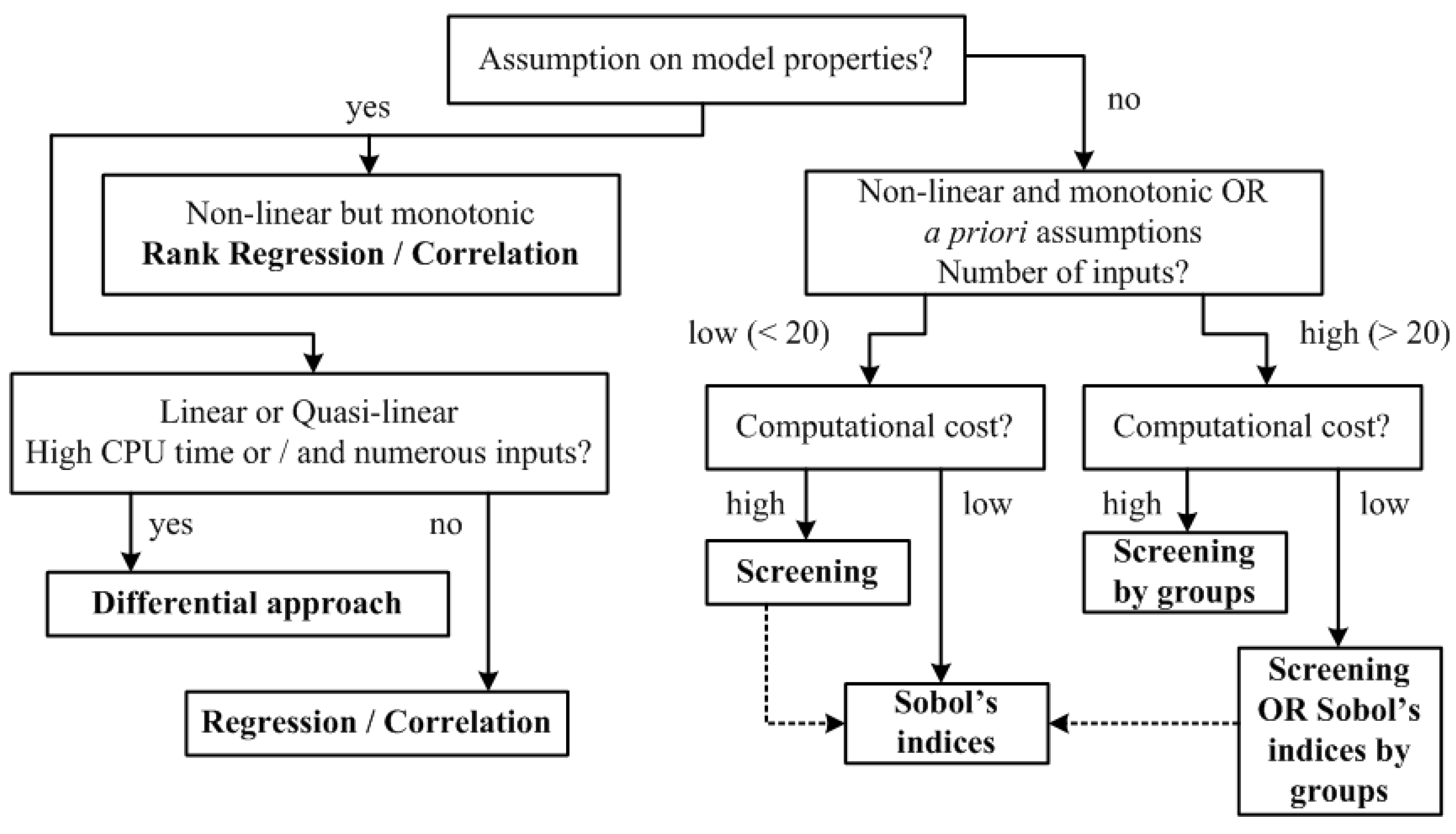
The techniques described above are common and are most-frequently used. The brief classification given in this article does not include many other approaches. They can be found, for example, in the case study [31], where the authors take into account the model structure, the number of inputs, and available computational resources to give a guide to how to use Sensitivity Analysis techniques (cf. Figure 1).
3. Analysis of Finite Fluctuations as an Approach to Sensitivity Measuring
This section is devoted to the introduction of the new technique and to the questions of its stability.
3.1. Technique Description
Analysis of Finite Fluctuations was introduced in study [22] as the sum of the results of an Economic Factor Analysis and concentrated mainly on the problem of how to manage resources effectively within existing conditions. Its primary issue is based on the initial model and creating a new model that links the finite fluctuation of the output to the finite fluctuations of inputs.
If fluctuations are small, in Mathematical Analysis, there exists the model of such connections. If the function describing the model is defined to be continuous and differentiable in a closed domain, the approximate relationship between the response and the small fluctuations of its arguments is
On the other hand, for some practical issues, fluctuations might be regarded as finite values rather than tiny ones.
When we use increments as finite fluctuations, there exists a model that is structurally exactly in the form connecting the finite fluctuation of the output and the inputs’ (factors) finite fluctuations. This is the Lagrange mean value theorem for functions, which is defined and continuous in a closed domain and has continuous partial derivatives inside this domain. It is formulated in the following manner:
Here, the mean (or intermediate) values of arguments (factors) are defined by the value of .
Let us have at the current moment of time factor initial state of Model (1) and the output . At the next moment of fixation, the factors of the system change and are described as and the output of the system is . Thus, the increment of the output can be defined, on the one hand, as the difference in the new and previous values of the outputs and, on the other hand, by the Lagrange theorem (7), i.e., the following equation can be composed and solved with respect to the parameter :
which allows estimation of the so-called factor loadings to obtain a model of the form
The procedure above is repeated m times (where m is the number of available observations); the numerical results of the analysis have to be averaged to construct the sensitivity measure [21].
3.2. Point-and-Interval Estimations of the Sensitivity Measure
Tukey’s weighted average can be used as an estimation of the mean value that is robust to outliers in the original data set. The algorithm for constructing this estimation is iterative and includes the following steps:
- Calculate the sample mean (the median is usually used at the beginning of the algorithm).
- Determine the distances from the calculated mean to each element of the sample. According to these distances, different weights are assigned to the sample elements, which are taken into account to recalculate the mean. The nature of the weight function is such that observations that are far enough away from the mean do not contribute much to the weighted mean.
Let be a sample from the calculated factor loadings for the input , is the sample median of the set , and S is the sample median of the set . For each element of the sample, the deviation from the mean is calculated
where c is a parameter that determines how sensitive the estimate is to outliers, and is a small value whose main purpose is to eliminate the possibility of dividing by zero.
To find the weight of each observation in the sample, we use a bi-quadratic function of the form
Tukey’s weighted estimate is
In addition to the point estimate of the mean, an interval is found to construct a value using the Student’s t-distribution approximation.
The symmetric confidence interval is given by
where is the -quantile of the Student’s t-distribution with the number of degrees of freedom .
3.3. Stability of the Proposed Technique
Inputs of Model (1) may have unrecoverable errors, which, nevertheless, should not cause inaccuracies when calculating estimates of the factor’s influence on the output. Stability of the numerical method is characterized by small deviations to the output value with insignificant changes to the inputs. Let the output value be found by the input value of the factor as a result of solving the problem. The input value has some error ; then, the output y has an error , so if at , , , the method is computationally stable.
For practical study of stability, it is necessary to conduct a series of computational experiments. The obtained corresponding samples consist of estimates of the significance of inputs and should be investigated from the point of view of similarity in the sense of mean values. For this purpose, we can formulate the null hypothesis about the shift of the mean values of the samples under the alternative hypothesis with the absence of such a shift, the test of which is further reduced to the calculation of some statistics (e.g., non-parametric Mann–Whitney–Wilcoxon test).
Let and be samples ordered in ascending order. To test the hypothesis, it is necessary to calculate
The Mann–Whitney U-statistic (12) defines the exact number of pairs of values and for which . Related to the U-statistic is the Wilcoxon statistic, which is defined as the sum of the ranks of elements of one sample (e.g., of volume ) in the total ordered sequence of elements of a joint sample (of volume ):
In the case when , the following approximation can be applied:
The statistic (13) is approximated by a normal distribution; the shift hypothesis (sample mean mismatch) is rejected with confidence if .
4. Numerical Example
In this section, we provide examples of applying the newly proposed approach to assess sensitivity measures of the factors of a neural network model. The first example is synthetic and is based on the well-known extended data set from the NeuralNetTools package of the R language, and the second example uses real indicators of healthcare data provided by the Compulsory Medical Insurance Fund of the Lipetsk region.
4.1. Neuraldat Data Set: Design of the Experiment
To assess the adequacy of the results obtained using the proposed approach, a series of computational experiments were conducted. The neuraldat data set from the NeuralNetTools package of the R data processing environment was used as data. The set contains 2000 realizations, which allows us to obtain 1999 finite response increments and their corresponding arguments. The described data set contains three independent and two dependent variables (only one dependent variable was used as an output for model-building and research at this stage). For numerical experiments, the number of independent variables was increased to 15 according to the scheme given in Table 1.
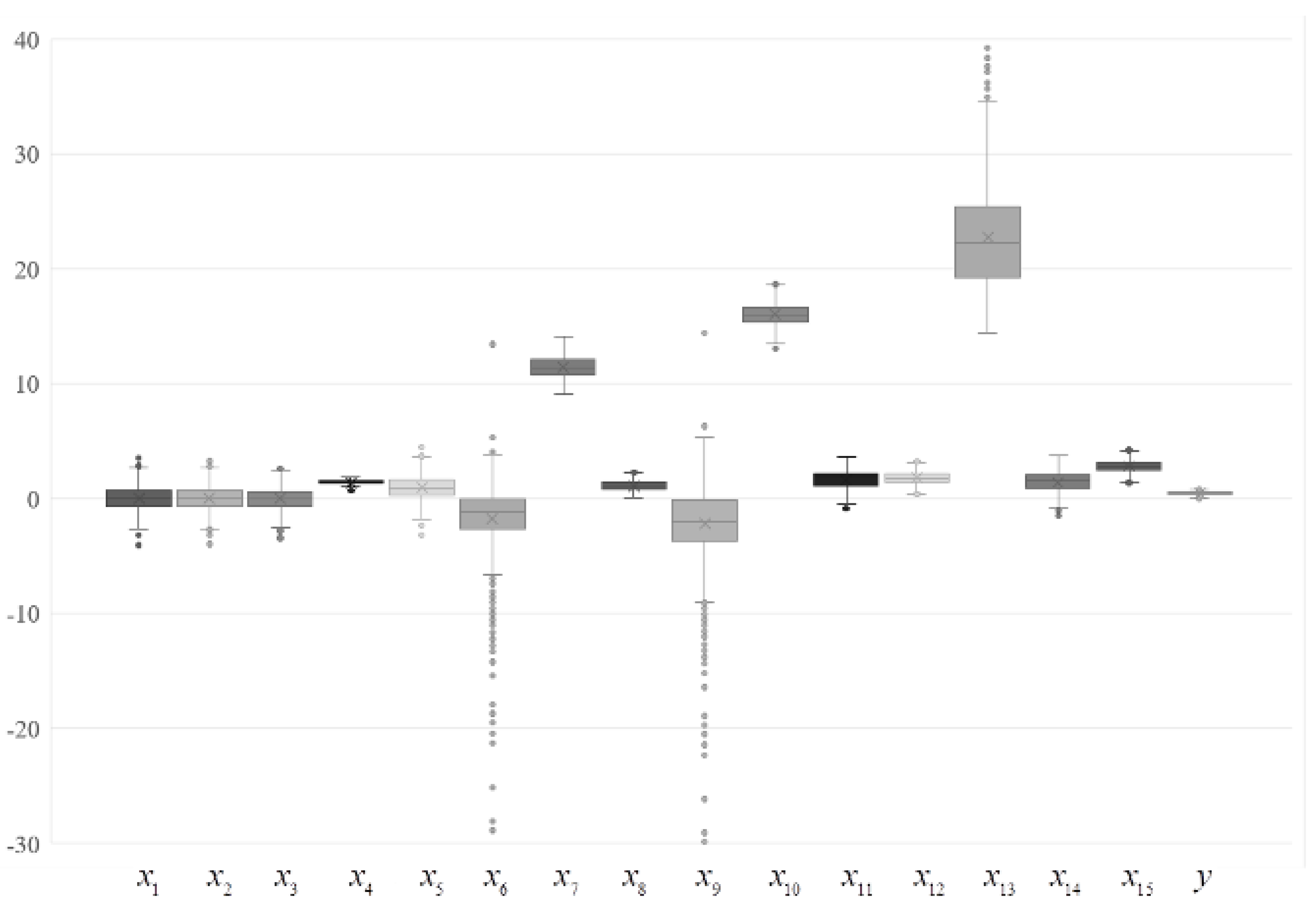
The independent variables obtained additionally represent series of random numbers with different statistical distributions (normal and Weibull distributions) and different values of these distribution parameters. The box-plots shown in Figure 2 demonstrate the spreads for the independent and dependent variables.
A neural network model with one hidden layer consisting of three neurons with the following structure was used as a model for the numerical experiment:
where is the response value; is a vector of factors; and are weight coefficients of the output and hidden layers, respectively; and are biases of the output and hidden layers, respectively; are logistic activation functions.
For the initial data set and the model used, MAE is 0.092%, which indicates high accuracy of the proposed neural network model and allows us to continue numerical experiments to find the sensitivity of Model (14).
4.2. Neuraldat Data Set: Discussion of Results
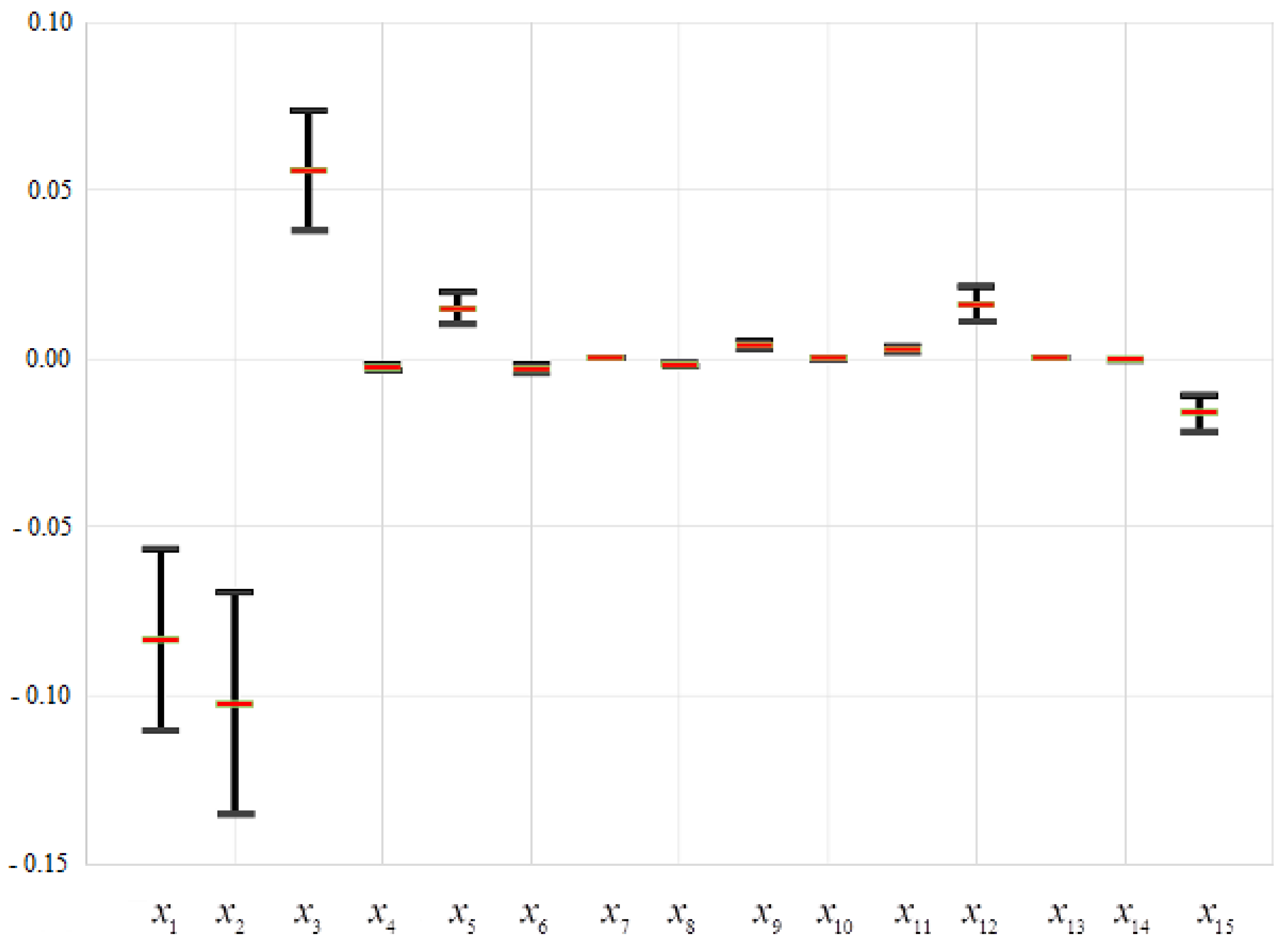
The calculated values of the sensitivity measures (Section 3) (point estimates obtained as Tukey’s weighted averages (10) and interval estimates (11)) for the described data set are presented in Figure 3.
According to the obtained results, the variables , , , , , and have the highest sensitivity. It should also be noted that the approach for analyzing the sensitivity of the model based on using Analysis of Finite Fluctuations, in addition to the strength of the influence of factors, assesses the direction of this influence. Thus, for Model (14), the factors , , and have a positive influence on the output y, while the factors , , and influence negatively.
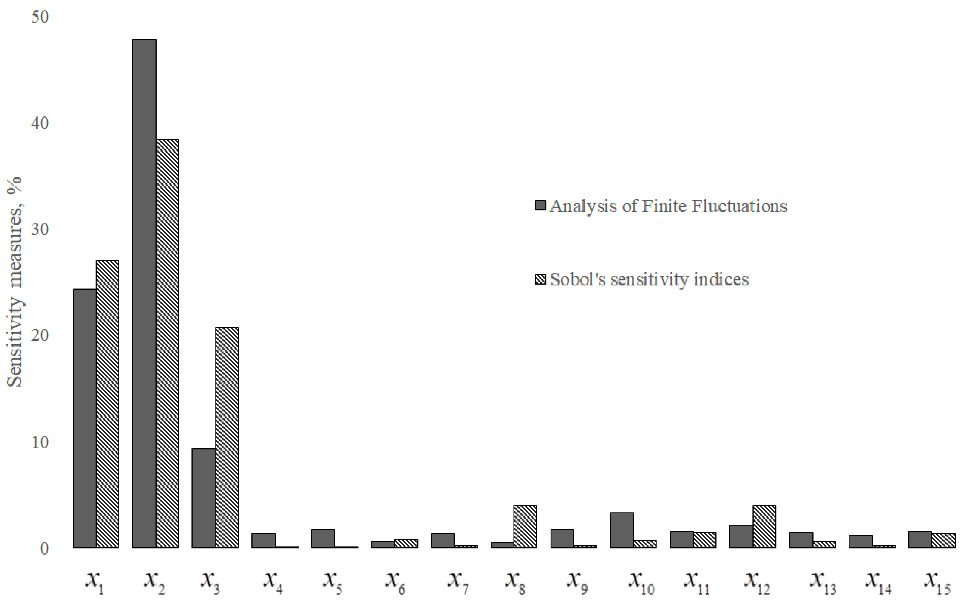
Figure 4 presents a comparison of the assessed sensitivity measures by analyzing final fluctuations in the factor loadings in accordance with the proposed approach, followed by finding Tukey’s weighted average for each factor loading and by using the algorithm for finding Sobol’s sensitivity indices. Analyzing the obtained results, we can state that both presented methods give similar results. It should be noted that due to the difference of scales used in different methods, the results of all methods were presented as percents.
When investigating the computational stability of the proposed approach, the approach described above was applied (Mann–Whitney–Wilcoxon statistics were calculated). For all analyzed input factors, the calculated values of the Mann–Whitney–Wilcoxon criterion exceed the tabular values. Thus, it is possible to reject the hypothesis about the presence of a shift between the mean values in the samples formed from the estimates of the influence of factors on the model output in the case of random fluctuations and without it.
4.3. Medical Healthcare Data: Design of Experiment
The data set of medical healthcare in the Lipetsk region includes 34 indicators. Data were collected from February to May 2019 and show how medical care was provided in more than 1 billion cases; one patient could be linked to many records (according to their visits to the physician). All the indicators could be divided into consolidated groups: indicators belonging to the patient, indicators belonging to the medical organization providing healthcare, indicators belonging to the disease, indicators belonging to the doctor, and indicators belonging to the particular case of medical care. It should be noted that assessing sensitivity in this task was a particular problem prior to building a neural network binary classifier to detect anomalies in data collected from hospitals. The initial neural network model with 34 input factors, 1 hidden layer with 3 neurons, and 1 output was investigated; logistic activation functions were used, and the reduced model uses the 15 most-important inputs (with the highest sensitivity measures), as presented in Table 2.
4.4. Medical Healthcare Data: Sensitivity Measures and Outlier Prediction
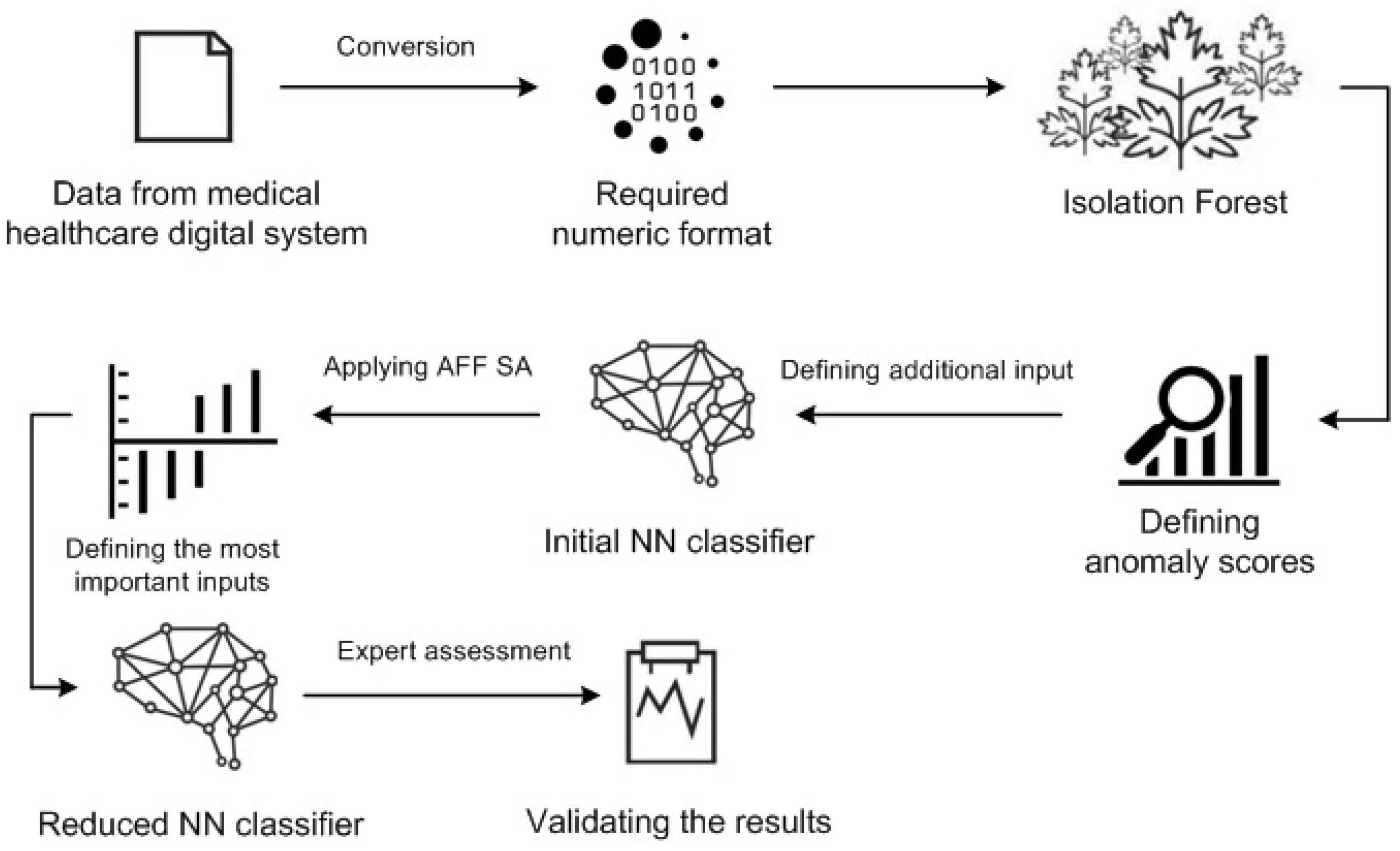
Since the model of a neural network must be reduced according to its input in order to increase the accuracy of the model, it is proposed to increase the results (distortion) of the isolation forest algorithm used to expand the input. This step has been optimized and is the basis for integrating error detection methods in the clinical setting described in [32]. The suggested workflow is shown in Figure 5.
The data for numerical testing are divided into two groups, 80% of which make up the training set and 20% the testing set. The final curtailed results showed an accuracy of 78%, with a type I error of 24% and a type II error of 16%. Analyzing the results of the outliers detected by the neural network model, it is found that most of the outliers are different from normal records. Most of the items identified fall into one of the following categories: First, in most established records, there are technical errors in the labels, such as record “chronic disease” instead of “dental consultation”. Second, minor ailments often require multiple visits to the doctor, such as five visits to the dentist to treat enamel degradation.
5. Conclusions and Future Work
In the article, the classification of existing methods of sensitivity assessment by factors of mathematical models is given. The Analysis of Finite Fluctuations approach based on the Lagrange mean value theorem is described and investigated. The only limitation to the proposed technique is that the model under consideration must be differentiable. The proposed method is compared with the calculation of Sobol’s indices; as a result, the consistency of the method is shown. The numerical stability of the procedure is investigated. Compared to the existing approaches, our technique does not use approximation of the original model; thus, it does not cause inaccuracy of the obtained results. The approach permits the interconnection between factors; the only limitation is the existence of the first partial derivatives. Our technique also takes into account all available information related to both the factors and the parameters of the initial model, which makes the obtained results of the analysis sustainable.
The next stage of the study is connected with applying the proposed technique to models that are convolutions of functions. Such functions can be used to model complicated hierarchical systems and multi-stage processes.
Funding
This research received no external funding.
Institutional Review Board Statement
Not applicable.
Informed Consent Statement
Not applicable.
Data Availability Statement
Simulated dataset for function examples used in numerical study is public and can be found at https://rdrr.io/cran/NeuralNetTools/man/neuraldat.html (accessed on 11 August 2023). Data on medical healthcare in the Lipetsk region was provided by the Compulsory Medical Insurance Fund of the Lipetsk region.
Acknowledgments
The author is deeply thankful to his scientific advisor, Semen Blyumin (1942–2023).
Conflicts of Interest
The author declares no conflict of interest.
References
- Saltelli, A.; Ratto, M.; Andres, T.; Campolongo, F.; Cariboni, J.; Gatelli, D.; Saisana, M.; Tarantola, S. Global Sensitivity Analysis: The Primer; John Wiley & Sons: Chichester, UK, 2008. [Google Scholar]
- Saltelli, A.; Tarantola, S.; Campolongo, F. Sensitivity analysis as an ingredient of modeling. Stat. Sci. 2000, 15, 377–395. [Google Scholar]
- Sobol, I.M. Global sensitivity indices for nonlinear mathematical models and their Monte Carlo estimates. Math. Comput. Simul. 2001, 55, 271–280. [Google Scholar] [CrossRef]
- Sanchez, D.G.; Lacarriere, B.; Musy, M.; Bourges, B. Application of sensitivity analysis in building energy simulations: Combining first-and second-order elementary effects methods. Energy Build. 2001, 68, 741–750. [Google Scholar] [CrossRef] [Green Version]
- Lamboni, M.; Kucherenko, S. Multivariate sensitivity analysis and derivative-based global sensitivity measures with dependent variables. Reliab. Eng. Syst. Saf. 2021, 212, 107519. [Google Scholar] [CrossRef]
- Borgonovo, E.; Castaings, W.; Tarantola, S. Model emulation and moment-independent sensitivity analysis: An application to environmental modelling. Environ. Model. Softw. 2012, 34, 105–115. [Google Scholar] [CrossRef]
- Rana, S.; Ertekin, T.; King, G.R. An efficient assisted history matching and uncertainty quantification workflow using Gaussian processes proxy models and variogram based sensitivity analysis: GP-VARS. Comput. Geosci. 2018, 114, 73–83. [Google Scholar] [CrossRef]
- Gul, R.; Schütte, C.; Bernhard, S. Mathematical modeling and sensitivity analysis of arterial anastomosis in the arm. Appl. Math. Model. 2016, 40, 7724–7738. [Google Scholar] [CrossRef]
- Zhang, Z.; Gul, R.; Zeb, A. Global sensitivity analysis of COVID-19 mathematical model. Alex. Eng. J. 2021, 60, 565–572. [Google Scholar] [CrossRef]
- Azizi, T.; Mugabi, R. Global Sensitivity Analysis in Physiological Systems. Appl. Math. 2020, 11, 119–136. [Google Scholar] [CrossRef]
- Hamby, D.M. A review of techniques for parameter sensitivity analysis of environmental models. Environ. Monit. Assess. 1994, 32, 135–154. [Google Scholar] [CrossRef]
- Sarrazin, F.; Pianosi, F.; Wagener, T. Global Sensitivity Analysis of environmental models: Convergence and validation. Environ. Model. Softw. 2016, 79, 135–152. [Google Scholar] [CrossRef] [Green Version]
- Ratto, M.; Castelletti, A.; Pagano, A. Emulation techniques for the reduction and sensitivity analysis of complex environmental models. Environ. Model. Softw. 2012, 34, 1–4. [Google Scholar] [CrossRef]
- Briggs, A.; Sculpher, M.; Buxton, M. Uncertainty in the economic evaluation of health care technologies: The role of sensitivity analysis. Health Econ. 1994, 3, 95–104. [Google Scholar] [CrossRef]
- Levine, R.; Renelt, D. A sensitivity analysis of cross-country growth regressions. Am. Econ. Rev. 1992, 82, 942–963. [Google Scholar]
- Jain, R.; Grabner, M.; Onukwugha, E. Sensitivity analysis in cost-effectiveness studies: From guidelines to practice. Pharmacoeconomics 2011, 29, 297–314. [Google Scholar] [CrossRef]
- Gosselin, C.; Isaksson, M.; Marlow, K.; Laliberte, T. Workspace and sensitivity analysis of a novel nonredundant parallel SCARA robot featuring infinite tool rotation. IEEE Robot. Autom. Lett. 2016, 1, 776–783. [Google Scholar] [CrossRef]
- Orekhov, A.L.; Ahronovich, E.Z.; Simaan, N. Lie group formulation and sensitivity analysis for shape sensing of variable curvature continuum robots with general string encoder routing. IEEE Trans. Robot. 2023, 39, 2308–2324. [Google Scholar] [CrossRef]
- VanderWeele, T.J.; Ding, P. Sensitivity analysis in observational research: Introducing the E-value. Ann. Intern. Med. 2017, 167, 268–274. [Google Scholar] [CrossRef] [Green Version]
- Carter, E.C.; Schönbrodt, F.D.; Gervais, W.M.; Hilgard, J. Correcting for bias in psychology: A comparison of meta-analytic methods. Adv. Methods Pract. Psychol. Sci. 2019, 2, 115–144. [Google Scholar] [CrossRef] [Green Version]
- Sysoev, A.; Ciurlia, A.; Sheglevatych, R.; Blyumin, S. Sensitivity analysis of neural network models: Applying methods of analysis of finite fluctuations. Period. Polytech. Electr. Eng. Comput. Sci. 2019, 63, 306–311. [Google Scholar] [CrossRef]
- Blyumin, S.L.; Borovkova, G.S.; Serova, K.V.; Sysoev, A.S. Analysis of finite fluctuations for solving big data management problems. In Proceedings of the 2015 9th International Conference on Application of Information and Communication Technologies (AICT), Rostov-on-Don, Russia, 14–16 October 2015. [Google Scholar]
- Pujol, G. Simplex-based screening designs for estimating metamodels. Reliab. Eng. Syst. Saf. 2009, 94, 1156–1160. [Google Scholar] [CrossRef] [Green Version]
- Hamby, D.M. A comparison of sensitivity analysis techniques. Health Phys. 1995, 68, 195–204. [Google Scholar] [CrossRef] [PubMed] [Green Version]
- Box, G.E.; Meyer, R.D. An analysis for unreplicated fractional factorials. Technometrics 1986, 28, 11–18. [Google Scholar] [CrossRef]
- Dean, A.; Lewis, S. Screening: Methods for Experimentation in Industry, Drug Discovery, and Genetics; Springer Science & Business Media: Berlin/Heidelberg, Germany, 2006. [Google Scholar]
- Hoeffding, W. A class of statistics with asymptotically normal distributions. Ann. Math. Stat. 1948, 13, 293–325. [Google Scholar] [CrossRef]
- Sobol, I.M. Sensitivity estimates for non linear mathematical models. Math. Comput. Exp. 1993, 1, 407–414. [Google Scholar]
- Efron, B.; Stein, C. The jacknife estimate of variance. Ann. Stat. 1981, 9, 586–596. [Google Scholar] [CrossRef]
- Homma, T.; Saltelli, A. Importance measures in global sensitivity analysis of non linear models. Reliab. Eng. Syst. Saf. 1996, 52, 1–17. [Google Scholar] [CrossRef]
- Meloni, C.; Dellino, G. (Eds.) A review on global sensitivity analysis methods. In Uncertainty Management in Simulation-Optimization of Complex Systems: Algorithms and Applications; Springer: Berlin/Heidelberg, Germany, 2015; pp. 101–122. [Google Scholar]
- Sysoev, A.; Scheglevatych, R. Combined approach to detect anomalies in health care datasets. In Proceedings of the 2019 1st International Conference on Control Systems, Mathematical Modelling, Automation and Energy Efficiency (SUMMA), Lipetsk, Russia, 20–22 November 2019. [Google Scholar]
Figure 1.
Brief classification of Sensitive Analysis techniques.

Figure 2.
Variations to output and input factors.

Figure 3.
Assessed sensitivity measures of Model (14) (presented are Tukey’s weighted average values and corresponding intervals).
Figure 3.
Assessed sensitivity measures of Model (14) (presented are Tukey’s weighted average values and corresponding intervals).

Figure 4.
Comparison of assessed sensitivity measures.

Figure 5.
Workflow of the proposed solution.


Table 1.
Test data characteristics.
| Input Factor | Characteristic |
|---|---|
Table 2.
Indicators with the highest impact on the neural network output.
| Name of the Indicator | Explanation | Sensitivity Measure, % |
|---|---|---|
| lPU_P | The name of the medical organization to which the patient is assigned | 4.11 |
| USL_OK | Conditions for the provided medical care | 8.25 |
| SROK_LECH | The length of the treatment or hospitalization | 6.29 |
| CEL_OBSL | The purpose of the patient’s appeal to the medical organization | 3.92 |
| PRVS | The doctor’s specialization | 4.08 |
| SPEC_END | The regional localization of the doctor’s specialization | 4.82 |
| POVTOR | The sign of a repeated treatment case for a single disease | 5.71 |
| TYPE_MN | The nature of the basic disease | 4.55 |
| ITAP | The stage of the medical examination or the preventive examination | 4.24 |
| RSLT_D | The result of the medical examination or the preventive examination | 4.77 |
| OBR | The indicator characterizing the method of payment for medical care in case of outpatient treatment | 3.15 |
| RAZN_SKOR | The time between calling for an ambulance and the arrival of medical services | 5.75 |
| VIDTR | The type of injury | 4.39 |
| NAZ_PK | The profile of around-the-clock or daily hospital for which a referral for the hospitalization was given based on the results of medical examination for patients of the 3rd health group | 5.33 |
| ANOMALY_SCORE | The anomaly score obtained by applying the Isolation Forest algorithm | 2.85 |
Disclaimer/Publisher’s Note: The statements, opinions and data contained in all publications are solely those of the individual author(s) and contributor(s) and not of MDPI and/or the editor(s). MDPI and/or the editor(s) disclaim responsibility for any injury to people or property resulting from any ideas, methods, instructions or products referred to in the content. |
© 2023 by the author. Licensee MDPI, Basel, Switzerland. This article is an open access article distributed under the terms and conditions of the Creative Commons Attribution (CC BY) license (https://creativecommons.org/licenses/by/4.0/).
Share and Cite
MDPI and ACS Style
Sysoev, A. Sensitivity Analysis of Mathematical Models. Computation 2023, 11, 159. https://doi.org/10.3390/computation11080159
AMA Style
Sysoev A. Sensitivity Analysis of Mathematical Models. Computation. 2023; 11(8):159. https://doi.org/10.3390/computation11080159
Chicago/Turabian StyleSysoev, Anton. 2023. "Sensitivity Analysis of Mathematical Models" Computation 11, no. 8: 159. https://doi.org/10.3390/computation11080159
Note that from the first issue of 2016, this journal uses article numbers instead of page numbers. See further details here.