Mathematical Modeling for Estimating the Risk of Rice Farmers’ Losses Due to Weather Changes

Abstract

This paper discusses the relationship between weather and rice productivity modeled using the Cobb–Douglas production function principle, with the hypothesis that rice production will increase in line with the increase in average rainfall, wind speed, and temperature every month and then decrease if the weather conditions exceed the threshold. As a result, farmers have the risk of losing rice production. To overcome this problem, we try to estimate the value of the risk. The purpose of this study is to estimate the risk of losses that occurred in rice plants due to weather changes. The method used in this study is risk estimation with the Tail Value at Risk (TVaR) approach. In addition to TVaR, it is estimated simultaneously with Value at Risk (VaR) and Conditional Value at Risk (CVaR). This study uses weather data consisting of rainfall data, wind speed, and air temperature collected from geophysical and meteorological data. Meanwhile, yield data were obtained and processed from the Central Statistics Agency and the West Java Agricultural Service. The data used are data from 2008 to 2021. There are two main parts of the results in this study, namely mathematical analysis and data analysis. The mathematical analysis is a risk model derivation process, which includes TVaR risk measurement. The data analysis process is a simulation of the estimated risk of rice production loss. The results obtained from this study are the value of opportunity risk of loss based on the VaR, CVaR, and TVaR approaches. The conclusion of this study is that the rice plants have a risk of loss in the form of reduced yields caused by weather changes. Farmers can plan to overcome this loss problem, by setting up a reserve fund. Risk of loss can be managed through the rice agricultural insurance program. This is in line with the Indonesian government’s program through the ministry of agriculture. Thus, farmers, insurance companies, and the government can manage the risk of losing rice yields.

1. Introduction

Agriculture is a type of business that is widely used with a low level of risk. Sources of risk are external or cannot be controlled by farmers, which generally come from the natural environment [1,2,3]. One of the main types of agriculture in Indonesia is food crops in the form of rice plants. Rice production in Indonesia often suffers losses due to crop failure. It is influenced by several factors, including drought, flooding, and plant pests [4,5,6,7]. To minimize losses due to crop failure, it is necessary to estimate the risk of these losses. One of the risk measurement tools is to use Tail Value at Risk (TVaR). However, to estimate TVaR, we have to estimate Value at Risk (VaR) and Conditional Value at Risk (CVaR). Thus, in this paper, we estimate the three risk measures.

Rice yields are influenced by several things, including business capital (in the form of labor, fertilizers, pesticides, etc.) and weather (in the form of rainfall, wind speed, and temperature) [2,8]. The working capital in this study is assumed to be constant (Cateris Paribus). Meanwhile, the weather is a risk factor that cannot be controlled by farmers. This study develops a risk model for rice production losses due to weather effects. As a preliminary study, we refer to the following papers. Based on the research results of Sheehy et al. (2006) [9], rice production is influenced by weather changes, rainfall, wind speed, and temperature.

The risk of loss in rice production occurs due to weather changes which have the potential risk to cause a decrease in the production yields obtained by farmers, compared to the expected average production amount [10,11,12,13,14,15]. Data on rice production are used as a reference for risk modeling. Risk is estimated based on predictions from crop yields and weather data [9,16]. The method used for the prediction and analysis of production results is usually a linear regression model [1,17]. Meanwhile, in this study, the Cobb–Douglas principle is used to predict the amount of production [18,19]. The Cobb–Douglas model is a production function model that shows the relationship between physical output (output) and production factors (input). All resources are assumed to be finite, but the weather has unlimited characteristics, which cannot be controlled by farmers. However, the variables of rainfall, temperature, and wind speed have unlimited values. The Cobb–Douglas model was chosen, with the hypothesis that rice production will increase with increasing rainfall, wind speed, and temperature. This is because rice plants need sufficient water, wind speed, and temperature. On the other hand, if it is too high or too low, it will cause a decrease in production output and will cause large losses [20,21,22,23,24]. This model is used to predict production yields with the hypothesis that rainfall increase, temperature, and wind speed results in production increase, however, this increase will reach a certain limit. If it is too high or too low, productivity will decrease. There will be situations where yields do not break even on production costs.

2. Literature Review

Previous related studies are as follows, Khai and Yabe (2011) [25] conducted a study on the measurement of agricultural production efficiency to determine the level of household efficiency in farming activities, using the stochastic frontier analysis method on the Cobb-Douglas production function. This study shows that the most important factors that have a positive impact on the level of technical efficiency are intensive labor, irrigation, and education. Nantui et al. (2012) [26] conducted a study to estimate the adaptive capacity of farmers to climate change adaptation strategies and their effects on paddy production in the Northern Region of Ghana. To measure the effect of farmers’ adaptive capacity on paddy production, the Cobb–Douglas production function double logarithmic regression model was used. The results of his research showed that the more farmers have the ability to adapt to climate changes, the more rice yields are obtained. Farmers should be empowered through extension in order to achieve a high adaptive capacity status, so it can help them obtain more rice yields. Ghoshal and Goswami (2017) [18] conducted a study on the production efficiency of agricultural systems in four regions of India. The stochastic production limit model uses panel data, which are used to estimate variations in efficiency by considering the integrated effects model. The results obtained, namely, the variables that are statistically significant and explain inefficiency in agricultural production are credit, irrigation, and fertilizer consumption. Nikkah et al. (2016) [27] conducted a study using the Life Cycle Assessment method and Cobb–Douglas modeling to determine the impact of phosphate and potassium fertilizers on kiwi fruit yields. From the results of the analysis, it is recommended to replace urea with other nitrogen fertilizer sources that have a lower environmental impact. Other studies that discuss the Cobb–Douglas method in the agricultural sector include [28,29,30,31,32,33,34].

Based on the results of the literature review, there is a research gap that is discussed in this study. Likewise, research has been carried out on the risk of loss in rice farming. Thus, we took three main keywords, namely prediction of rice production, risk of loss, and weather. This result is used as a research gap, so the topic is “Mathematical Modeling for Estimating the Risk of Rice Farmers’ Losses Due to Weather Changes”.

The research question (RQ) of this paper is formulated as follows: how to manage financial risk in rice farming? The scope of this research is financial loss risk management in rice farming. Meanwhile, the risk factors in this paper are for weather conditions (rainfall, temperature, and wind speed) limited only to the West Java area. However, we formulate a risk model and estimate the risk of loss in rice farming which can be applied flexibly in other areas with similar natural conditions.

3. Materials and Methods

Materials are data objects used in research, while methods consist of models used in analyzing data. The descriptions of materials and methods in this study are described below sequentially.

3.1. Materials

In this paper, to formulate a risk model for rice farming losses, Value at Risk (VaR), Conditional Value at Risk (CVaR), and Tail Value at Risk (TVaR) are used. The scope of this research is risk management of rice farming losses. This study uses weather data consisting of rainfall, wind speed, and air temperature data collected from geophysical and meteorological data. Meanwhile, yield data were obtained and processed from the Central Statistics Agency and the West Java Agricultural Service. The data used are data from 2008 to 2021. Considering the weather data in Indonesia, especially Bandung Regency, West Java, is different every month, the presentation of the data is grouped by month. The recorded data consist of rice productivity, wind speed, temperature, and rainfall data. The summary of the data used are presented in Appendix D. The processed data were obtained over a period of approximately 14 years. In this paper, data analysis of weather variables on rice production (Q) is carried out as the dependent variable. Weather variables, which consist of wind speed (X₁), average temperature (X₂), and rainfall (X₃), then act as independent variables. Appendix D displays the processed data, which are data above the threshold. The threshold in this case is chosen by the principle of Peaks Over Threshold (POT).

3.1.1. Risk Model

Risk is a hazard that can occur as a result of going process or future events [23]. In the field of insurance, risk can be defined as a state of uncertainty, where if an undesirable situation occurs, it can cause a loss. There are several forms of risk, including pure risk, speculative risk, particular risk, and fundamental risk. Here is a brief explanation [35].

• Pure risk is a risk that results in only two types: loss or break even, for example, theft, accident, or fire.
• Speculative risk is a risk that results in three types: loss, profit or break even, for example, gambling.
• Particular risks are risks that come from individuals and local impacts, for example, plane crashes, car crashes, and ship aground.
• Fundamental risk is a risk that does not come from individuals and the impact is wide, for example, hurricanes, earthquakes, and floods.

The risks raised in this paper are fundamental risks. The object of observation is the risk of the impact of weather on the amount of rice yields. The next sub-chapter briefly discusses rice plants.

3.1.2. Rice Plants

Rice is one of the most important cultivated plants in human civilization. Rice refers to the type of cultivated plant. Rice is thought to come from India or Indochina and entered Indonesia brought by ancestors who migrated from mainland Asia around 1500 BC. [36,37].

Several types of rice varieties, according to their habitat, included upland rice, swamp rice, pera rice, sticky rice, and pandan wangi rice [38].

Upland Rice

Upland rice is developed in rainfed areas. This type of rice is relatively tolerant without flooding as in rice fields. Usually, upland rice is grown using an intercropping system. In the intercropping system, not only rice but also other crops are grown in one area. Upland rice is usually intercropped with corn or cassava.

Swamp Rice

Swamp rice or tidal rice grows wild and is cultivated in swampy areas. Swamp rice is able to form long stems so that it can follow extreme seasonal changes in water depth.

Pera Rice

Rice grains when cooked do not stick together. This classification is mainly seen from the consistency of the rice.

Sticky Rice

Sticky rice is often called glutinous rice. It has been known for a long time. Glutinous rice has amylose content below 1% in its rice starch. Starch is dominated by amylopectin, so when cooked it is very sticky.

Pandan Wangi Rice

Pandan wangi rice was developed by people in several places in Asia, the famous one in Indonesia is the “Cianjur Pandanwangi” rice (it has now become a superior cultivar). This is a long-living javanica variety [36].

One of the most important stages in rice breeding is the release of the “IR5” and “IR8” cultivars, which are the first short-lived rice with high yield potential. This is the beginning of a change in rice cultivation. Subsequent rice cultivars generally have the “genes” of the two pioneer cultivars. From sub-Section 3.1.1, it is revealed that fundamental risk is a risk that does not come from individuals and has a wide impact, for example, hurricanes, earthquakes, and floods. Rice agricultural production is considered important in both developed and developing countries because of its role in providing food and rural employment [39,40].

3.1.3. Cobb–Douglas Production Function

The production function is an equation that describes the relationship between inputs and outputs, or what is used to make a particular product. the Cobb–Douglas production function is a special standard equation that is applied to describe how much of two or more inputs-outputs go into the production process, with capital and labor as inputs.

The Cobb–Douglas concept can be developed for the model of rice productivity by modifying several independent variables. For example, the Cobb–Douglas function of form (1) is modified into a Cobb–Douglas concept with elasticity developed with reference to the following forms.

$$Q=\beta X_1^{{\alpha }_1}{X}_2^{{\alpha }_2}{X}_3^{{\alpha }_3}{e}^u$$

(1)

where the rank in Equation (2) states the elasticity stated in the form of: ${\alpha }_i$ = ${\alpha }_i$ (I)

• $Q$: rice production per planting period (kg)
• $X_1$: rainfall (mm)
• $X_2$: temperature (°C)
• $X_3$: wind speed (m/s)
• $u$: random error
• $e$: natural logarithm.

Variable I, as the index is assumed to affect the elasticity significantly of production where the scale of business is defined ${\displaystyle \sum }_{1=1}^3 {\alpha }_i=1$. The effect of variable I can be tested if in the equation model (1) it becomes:

$$Q=\beta X_1^{{\alpha }_1\left(I\right)}{X}_2^{{\alpha }_2\left(I\right)}{X}_3^{{\alpha }_3\left(I\right)}{e}^u$$

(2)

The scale line in Equation (2) is no longer unique as in Equation (1) because there is a variable I that affects it, but they both pass through the origin (O).

Variable selection I can represent differences in size, level of management, capital or labor so that the production function is no longer homogeneous. Equation (2) can be written in the form of the following logarithmic linear equation:

$$\ln Q=\ln \beta +{\alpha }_1\left(I\right)\ln X_1+{\alpha }_2\left(I\right)\ln X_2+{\alpha }_3\left(I\right)\ln X_3+u,$$

(3)

assuming that ${\beta }_i$ is linear in its parameters, so the Ordinary Least Square (OLS) estimation can be used.

Each variable value will represent the partial elasticity of each independent variable with a unique production scale. While the value of ${\alpha }_i$ in the Cobb–Douglas equation is the elasticity of the input factors $X_1, X_2$, and $X_3$ respectively. In the Cobb–Douglas equation the amount of elasticity of the input factors can show the additional level of yield under the following conditions:

• If ${\displaystyle \sum }_{1=1}^3 {\alpha }_i=1$, there is a constant increase in returns to scale of production, (Scale of returns is constant).
• If ${\displaystyle \sum }_{1=1}^3 {\alpha }_i>1$, there is an increasing scale of return.
• If ${\displaystyle \sum }_{1=1}^3 {\alpha }_i<1$, there is an additional drop back to scale.

The Cobb–Douglas production model in Equation (1) follows the law of diminishing returns, meaning that initially, every increase in the value of a production factor will increase productivity until a certain value addition of a production factor will actually decrease productivity.

3.2. Methods

The methods used in this study to measure the risk of loss are risk measurement and Peak Over Threshold. The risk measurement included Value at Risk, Conditional Value at Risk, and Tail Value at Risk [41]. These measurements are explained as follows.

3.2.1. Risk Measurement

In this subsection, an analysis of the risks that occurred in the production process of rice farming caused by weather changes is carried out. It is suspected that extreme weather changes can affect rice yields. Rainfall, wind speed, and extreme temperature are also expected to increase the level of yield loss. The methods used to measure risk are Value at Risk, Conditional Value at Risk (CVaR), and Tail Value at Risk (TVaR), which are used to measure the risk of loss due to yield failure [42,43].

Value at Risk (VaR) is a statistic used to measure the extent of possible losses over a certain period of time [44]. This measure is used to determine the potential loss opportunities in a production process. Meanwhile, Conditional Value at Risk (CVaR), also known as shortfall expectation, is a risk assessment measure that quantifies the amount of tail risk that an asset’s return has. The CVaR value is derived from the VaR calculation, so assumptions such as the shape of the distribution of returns, threshold, the periodicity of the data, and assumptions about stochastic volatility will affect all the CVaR value. The CVaR value is calculated from VaR, which is the average value that is outside the VaR [45]. Meanwhile Tail Value at Risk (TVaR), is a measure to quantify the value of the expected loss from an event beyond a certain probability level. This measure of risk is also known as Mean Excess Loss, Mean Shortfall, or Tail Value at Risk [45].

The mathematically constructed risk measure is determined as follows. Let X be a continuous random variable with a loss distribution function $F_X\left(x\right)$, the risk value at the probability level $\alpha$ $(0<\alpha <1$), denoted by $Va{R}_{\alpha }\left(X\right)$, is the quantile of X, that is,

$$Va{R}_{\alpha }\left(X\right)=F_X^{-1}\left(\alpha \right)=x_{\alpha }$$

(4)

If $\alpha$ is close to 1 (0.95 or 0.99), then the probability of X’s loss exceeding $Va{R}_{\alpha }\left(X\right)$ is not more than $1-\alpha$, which is quite small. The value of VaR at the probability level $\alpha$ as $Va{R}_{\alpha }\left(X\right)$ when the variable loss occurs. Alternatively, if $F_X\left(x\right)$ is a ladder function (X is a discrete random variable), then there is some ambiguity in defining $F_X^{-1}\left(\alpha \right)$, so the definition of $Va{R}_{\alpha }\left(X\right)$ can be expressed as

$$Va{R}_{\alpha }\left(X\right)=\inf \left\{x\in \left[0,\infty \right):F_X\left(x\right)\ge \alpha \right\}.$$

(5)

Meanwhile, the weakness of VaR is that it does not use information about the tail distribution. While TVaR with probability $\alpha$, denoted by $TVa{R}_{\alpha }\left(X\right)$ is defined as

$$TVa{R}_{\alpha }\left(X\right)=E\left(X|X>x_{\alpha }\right)$$

(6)

If X is a continuous random variable, then Value at Risk is written as

$$TVa{R}_{\alpha }\left(X\right)=E\left[X|X>Va{R}_{\alpha }\left(X\right)\right]$$

as a measure of risk. If the loss exceeds the VaR condition or the excess loss, then the risk is in the form

$$\left[X-Va{R}_{\alpha }\left(X\right)\right]|X>Va{R}_{\alpha }\left(X\right)$$

The average of this conditional excess is called the conditional VaR, which is denoted by $CVa{R}_{\alpha }\left(X\right)$ and is defined as

$$CVa{R}_{\alpha }\left(X\right)=E[X-Va{R}_{\alpha }\left(X\right)| X > Va{R}_{\alpha }\left(X\right)]$$

(7)

Equation (7) can be written as

$$\begin{gathered} CVa{R}_{\alpha }\left(X\right)=E [X|X>Va{R}_{\alpha }\left(X\right)\left]-E\right[Va{R}_{\alpha }\left(X\right)|X>Va{R}_{\alpha }\left(X\right)] \\ =TVa{R}_{\alpha }\left(X\right)-Va{R}_{\alpha }\left(X\right) \end{gathered}$$

(8)

If $Va{R}_{\alpha }$ is used as economic capital, then the lack of capital is the value of VaR, when X is continuous, i.e., $Va{R}_{\alpha }=x_{\alpha }$, and the mean shortfall is

$$\begin{gathered} E[{\left(X-x_{\alpha }\right)}_{+}\left]=E \right[X-x_{\alpha } | X>x_{\alpha }]Pr(X>x_{\alpha }) \\ =\left(1-\alpha \right)CVa{R}_{\alpha }, \end{gathered}$$

thus, we obtained

$$TVa{R}_{\alpha }=x_{\alpha }+CVa{R}_{\alpha }=x_{\alpha }+\frac{1}{1-\alpha }E[{\left(X-x_{\alpha }\right)}_{+}]$$

(9)

If X represents a random variable of loss, the tail value at risk X with a 100% confidence level, denoted TVaR(X) is the average loss that exceeds the 100 α percentile. The value of TVaR(X) can be written as

$$TVa{R}_{\alpha }=E\left(X|X>x_{\alpha }\right)=\frac{1}{1-\alpha }\underset{x_{\alpha }}{\overset{\infty }{{\displaystyle \int }}}x{f}_X\left(x\right)dx$$

(10)

If we let ξ = $F_X\left(x\right)$

$$\underset{x_{\alpha }}{\overset{\infty }{{\displaystyle \int }}}x{f}_X\left(x\right)dx=\underset{x_{\alpha }}{\overset{\infty }{{\displaystyle \int }}}xd{F}_X\left(x\right)dx=\underset{\alpha }{\overset{1}{{\displaystyle \int }}}{x}_{\mathsf{\xi }}d\mathsf{\xi }$$

then

$$TVa{R}_{\alpha }=E\left(X|X>x_{\alpha }\right)=\frac{1}{1-\alpha }\underset{\alpha }{\overset{1}{{\displaystyle \int }}}{x}_{\mathsf{\xi }}d\mathsf{\xi }=\frac{1}{1-\alpha }\underset{\alpha }{\overset{1}{{\displaystyle \int }}}Va{R}_{\mathsf{\xi }}d\mathsf{\xi }$$

(11)

So, $TVa{R}_{\alpha }$ can be interpreted as an average quantile that exceeds $x_{\alpha }$. If the number is finite, use part integration and substitution to rewrite it as

$$TVa{R}_{\mathsf{\alpha }}\left(X\right)=\frac{{{\displaystyle \int }}_{\alpha }^{1}Va{R}_{\mathrm{u}}\left(X\right)du}{\left(1-\alpha \right)}$$

(12)

Thus, TVaR can be seen as the average of all VaR values with a confidence level of $\alpha$. The TVaR value gives an indication of the tail of the distribution, not just VaR. Thus, TVaR can be seen as the average of all VaR values with a confidence level of $\alpha$.

$$\begin{gathered} TVa{R}_{\mathsf{\alpha }}\left(X\right)=E\left(X|X>\mathsf{\pi }\alpha \right) \\ =Va{R}_{\alpha }\left(\mathrm{X}\right)+\frac{{{\displaystyle \int }}_{{\mathrm{x}}_{\alpha }}^{\infty }\left(x-{\mathsf{\pi }}_{\alpha }\right)f\left(x\right)dx}{1-\alpha } \\ =Va{R}_{\mathsf{\alpha }}\left(X\right)+e\left({\mathsf{\pi }}_{\alpha }\right) \end{gathered}$$

(13)

where $e\left({\mathsf{\pi }}_{\alpha }\right)$ is the average excess loss function evaluated at the 100$\alpha$ percentile, TVaR is greater than VaR value. TVaR value is an extreme event that exceeds the VaR threshold. TVaR provides an excess of average losses in bad times, that is, the VaR threshold has been exceeded.

If the random loss variable X is assumed to be normally distributed with the mean $\mathsf{\mu }$, standard deviation $\mathsf{\sigma }$, and probability density function is

$$f\left(x\right)=\frac{1}{\mathsf{\sigma }\sqrt{2\mathsf{\pi }}}\exp \left[\frac{1}{2}{\left(\frac{x-\mathsf{\mu }}{\mathsf{\sigma }}\right)}^2\right]$$

(14)

Let $f\left(x\right)$ and $F\left(x\right)$ represent the probability density function and the cumulative distribution function of the standard normal distribution (μ = 0 and σ = 1) and

$$TVa{R}_{\mathsf{\alpha }}\left(X\right)=\mathsf{\mu }+\mathsf{\sigma }\frac{f [F^{-1}\left(\alpha \right)]}{1-\alpha }$$

(15)

In this case, the risk measure can be translated into the standard deviation principle.

In the case of an exponential distribution. Consider an exponential distribution with mean and probability density function

$$f\left(x\right)=\frac{1}{\mathsf{\theta }}\exp \left(-\frac{x}{\mathsf{\theta }}\right), x>0$$

so

$$Va{R}_{\mathsf{\alpha }}\left(X\right)=-\mathsf{\theta } \ln \left(1-\alpha \right)$$

and

$$TVa{R}_{\mathsf{\alpha }}\left(X\right)=Va{R}_{\mathsf{\alpha }}\left(X\right)+\mathsf{\theta }$$

(16)

The third is Pareto distribution with scale parameters and shape parameters are p > 1 and

$$F\left(x\right)=1-{\left(\frac{\mathsf{\theta }}{x+\mathsf{\theta }}\right)}^p, x>0$$

so

$$Va{R}_{\mathsf{\alpha }}\left(X\right)=\mathsf{\theta } [{\left(1-\alpha \right)}^{\frac{-1}{p}}-1$$

and

$$TVa{R}_{\mathsf{\alpha }}\left(X\right)=Va{R}_{\mathsf{\alpha }}\left(X\right)+\frac{Va{R}_{\mathsf{\alpha }}\left(X\right)+\mathsf{\theta }}{p-1}$$

(17)

Another advantage of TVaR over VaR is that linear increase function in VaR, which means that a mean excess loss greater than VaR indicates an increased hazard, where the results vary greatly depending on the choice of distribution.

Whereas the normal distribution has a tail lighter than the probability of extreme value leading to smaller quantiles. The Pareto distribution with $\mathsf{\xi }<1$, has a heavy tail, so it has relatively larger extreme quantiles.

Numerical values of VaR and TVaR can be done either from the data directly or from the distribution model. The quantile method of the empirical distribution can be used to estimate the VaR of the data. While TVaR is the expected value of observations that is greater than the given threshold because many observations exceed the threshold. In cases where there are not many observations exceeding the threshold, we prefer to obtain a model for the distribution of all observations, or at least all observations calculated directly from the fitted distribution. This can be done for a continuous distribution, using the relation.

3.2.2. Peak over Threshold

According to [1] the approach used to determine the extreme distribution it focuses on determining the probability value in the tail region. It can be used as extreme value theory (EVT). This theory is used to predict rare events. Meanwhile, the extreme value theory consists of the Block Maxima (BM) model and the Peak Over Threshold (POT) model. The BM model is a method used to find extreme data based on the highest value from each period (daily, weekly, monthly), while the POT model is a method used to estimate data based on values that exceed the threshold value. The POT method is an extreme data distribution that is the result of a generalization of the Pareto distribution known as the Generalized Pareto Distribution (GPD). In this case, we choose POT as the threshold.

The POT model is an extreme data distribution that is the result of a generalization of the Pareto distribution known as the Generalized Pareto Distribution (GPD). Generalized Pareto Distribution is the distribution limit for the distribution of extreme data that is above the threshold u. The limit of the function is the conditional distribution of the variable $Y=\left(X-u |X>u\right)$.

$$F\left(y\right)=1-{\left(1+\frac{\mathsf{\xi }\left(y\right)}{\mathsf{\sigma }}\right)}^{-\frac{1}{\mathsf{\xi }}}$$

(18)

where $\{y:y>0$ and $1+\frac{\mathsf{\xi }\left(y\right)}{\mathsf{\sigma }}>0\}$.

The density function of Equation (18) is

$$f\left(x;\mathsf{\sigma },\mathsf{\xi }\right)=\left\{\begin{array}{c}\frac{1}{\mathsf{\sigma }}{\left(1+\frac{\mathsf{\xi }x}{\mathsf{\sigma }}\right)}^{-\frac{1}{\mathsf{\xi }}-1}, \mathsf{\xi }\ne 0\\ \frac{1}{\mathsf{\sigma }}\exp \left(-\frac{x}{\mathsf{\sigma }}\right), \mathsf{\xi }=0\end{array}\right.$$

(19)

where domains $0\le x<\infty$ for $\mathsf{\xi }\ge 0$ and $0\le x<-\frac{\mathsf{\sigma }}{\mathsf{\xi }}$, for $\mathsf{\xi }<0$. This density function has two parameters, namely the form parameter $\left(\mathsf{\xi }\right)$ and the scale parameter $\left(\mathsf{\sigma }\right)$. Estimating GPD parameters in this discussion is used the maximum likelihood estimator. The estimated value is calculated numerically using the Newton Raphson method.

4. Results

The research results can be divided into two parts, namely the results of mathematical modeling and the results of data analysis. The two results were found to be congruent. The description is explained as follows.

4.1. Mathematical Modelling

This idea was developed from the research of Riaman et al. (2021) [5], which discussed a model of determining the premium of paddy insurance using the extreme value theory method and the operational value at risk approach. In this paper, a rice risk model based on yield productivity returns is developed, with a modified Cobb–Douglas concept. Meanwhile, this paper discusses productivity risk based on changes in production output. That is, by comparing the current production amount to the production one period back. The variable used is the production quantity $Q_t$.

For example, $Q_t$ representing the production of the growing season at time t and $Q_{t-1}$ the production of the growing season in the previous period. Referring to Equation (2), can be expressed as $\ln Q_t$

$$\ln Q_t=\ln \beta +{\alpha }_1\left(I\right)\ln X_{1t}+{\alpha }_2\left(I\right)\ln X_{2t}+{\alpha }_3\left(I\right)\ln X_{3t}+u_t$$

(20)

If we look at the production results from one period back, then Equation (20) can be written as follows

$$\ln Q_{t-1}=\ln \beta +{\alpha }_1\left(I\right)\ln X_{1t-1}+{\alpha }_2\left(I\right)\ln X_{2t-1}+{\alpha }_3\left(I\right)\ln X_{3t-1}+u_{t-1}$$

(21)

If Equation (20) is subtracted by Equation (21), then we get

$$\ln Q_t-\ln Q_{t-1}={\alpha }_1\left(I\right)\left[\ln X_{1t}-\ln X_{1t-1}\right]+{\alpha }_2\left(I\right)\left[\ln X_{2t}-\ln X_{2t-1}\right]+{\alpha }_3\left(I\right)\left[\ln X_{3t}-\ln X_{3t-1}\right]+u_t-u_{t-1}$$

(22)

Equation (22) using the logarithmic property can be expressed as Equation (23)

$$\ln \frac{Q_t}{Q_{t-1}}={\alpha }_1\left(I\right)\ln \frac{ X_{1t}}{ X_{1t-1}}+{\alpha }_2\left(I\right)\ln \frac{ X_{2t}}{ X_{2t-1}}+{\alpha }_3\left(I\right)\ln \frac{ X_{3t}}{ X_{3t-1}}+u_t-u_{t-1}$$

(23)

If $\ln \frac{Q_t}{Q_{t-1}}=R_{Q_t}$, represents return in period t, then

$$R_{Q_t}={\alpha }_{1}R{X}_{1t}+{\alpha }_{2}R{X}_{2t}+{\alpha }_{3}R{X}_{3t}+v_t$$

(24)

The mean of Equation (24) is

$$\begin{gathered} E\left[R_{Q_t}\right]={\alpha }_{1}E{R}_{X_{1t}}+{\alpha }_{2}E{R}_{X_{2t}}+{\alpha }_{3t}E{R}_{X_{3t}}+E\left[v_t\right] \\ {\mathsf{\mu }}_{Qt}={\alpha }_1{\mathsf{\mu }}_{X_{1t}}+{\alpha }_2{\mathsf{\mu }}_{X_{2t}}+{\alpha }_3{\mathsf{\mu }}_{X_{3t}}\mathrm{and} \left[v_t\right]=0. \end{gathered}$$

Completely written in a system of linear equations as Equation (25)

$$\begin{gathered} {\mathsf{\mu }}_{Q_1}={\alpha }_1{\mathsf{\mu }}_{X_{11}}+{\alpha }_2{\mathsf{\mu }}_{X_{21}}+{\alpha }_3{\mathsf{\mu }}_{X_{31}} \\ {\mathsf{\mu }}_{Q_2}={\alpha }_1{\mathsf{\mu }}_{X_{12}}+{\alpha }_2{\mathsf{\mu }}_{X_{22}}+{\alpha }_3{\mathsf{\mu }}_{X_{32}} \\ {\mathsf{\mu }}_{Q_3}={\alpha }_1{\mathsf{\mu }}_{X_{13}}+{\alpha }_2{\mathsf{\mu }}_{X_{23}}+{\alpha }_3{\mathsf{\mu }}_{X_{33}} \end{gathered}$$

(25)

In matrix form, we get Equation (26)

$$\left(\begin{array}{c}{\mathsf{\mu }}_{Q_1}\\ {\mathsf{\mu }}_{Q_2}\\ {\mathsf{\mu }}_3\end{array}\right)=\left(\begin{array}{ccc}{\alpha }_1& {\alpha }_2& {\alpha }_3\end{array}\right)\left(\begin{array}{ccc}{\mathsf{\mu }}_{X_{11}}& {\mathsf{\mu }}_{X_{12}}& {\mathsf{\mu }}_{X_{13}}\\ {\mathsf{\mu }}_{X_{21}}& {\mathsf{\mu }}_{X_{22}}& {\mathsf{\mu }}_{X_{23}}\\ {\mathsf{\mu }}_{X_{31}}& {\mathsf{\mu }}_{X_{32}}& {\mathsf{\mu }}_{X_{33}}\end{array}\right)$$

(26)

In vector form, it can be expressed as (27)

$$\begin{gathered} {\mathsf{\mu }}_{Qt}={\alpha }^T\mathsf{\mu } \\ {\alpha }^T=\left({\alpha }_1,{\alpha }_2,{\alpha }_3\right) \\ {\mathsf{\mu }}^T=\left({\mathsf{\mu }}_1,{\mathsf{\mu }}_2,{\mathsf{\mu }}_3\right) \end{gathered}$$

(27)

${\mathsf{\sigma }}_{Q_t}^2$: risk of crop failure is measured by variance.

If the risk of crop failure is measured by VaR, where ${\mathsf{\mu }}_{Qt}={\alpha }^T\mathsf{\mu }$, ${\alpha }^T=\left({\alpha }_1,{\alpha }_2,{\alpha }_3\right)$, and ${\mathsf{\mu }}^T=\left({\mathsf{\mu }}_{X_1},{\mathsf{\mu }}_{X_2},{\mathsf{\mu }}_{X_3}\right)$, then the following theorem appears.

Theorem 1.

If it is assumed that the relationship pattern of the three climatic factors in Equations (18) and (20) and the initial capital for rice planting is one unit and the risk is measured by Value at Risk, then

$$\begin{gathered} Va{R}_p\left(R_{Qt}\right)=-\left[{\mathsf{\mu }}_{R_{Qt}}+z_p{\mathsf{\sigma }}_{R_{Qt}}\right] \\ =-[{\alpha }^T{\mathsf{\mu }}_{R_{Qt}}+z_p\sqrt{{\alpha }^T\mathsf{\Omega }\alpha +v^{T}v}]. \end{gathered}$$

The proof of theorem is included in Appendix A.

The risk measure using VaR does not consider all possible worst-case scenarios, so it needs refinement, which in this case, can be used CVaR. CVaR is the average return for a more pessimistic tail risk measure when compared to VaR. The following theorem will provide an explanation of CVaR for the case of financial risk in rice farming.

Theorem 2.

If it is assumed that the relationship pattern of the three climatic factors in Equations (18) and (20) and the initial capital for rice planting is one unit and the risk is measured by value at risk, then

$$CVaR(R_{Qt})={{\displaystyle \int }}_{-\infty }^{Va{R}_p\left(Q_t\right)}\frac{1}{\sqrt{2\mathsf{\pi }}}\exp (-\frac{1}{2}{Q}_t^2)d{Q}_t.$$

The proof of theorem is included in Appendix B.

The next result, if the initial capital to plant rice is one unit and risk is measured by Value at Risk, then Tail Value at Risk is equivalent to Value at Risk plus Conditional Value at Risk.

Theorem 3.

If it is assumed that the relationship pattern of the three climatic factors in Equations (18) and (20) and the initial capital for rice planting is one unit and the risk is measured by value at risk, then

$$\mathit{TVaR}=Va{R}_{\mathsf{\alpha }}\left(R_{Qt}\right)+\frac{Va{R}_{\mathsf{\alpha }}\left(R_{Qt}\right)+\mathsf{\theta }}{\mathsf{\alpha }-1}.$$

The proof of theorem is included in Appendix C.

All of the above theorems are based on hypotheses based on plotting rice yield return data. From the plotting results, it is obtained that the distribution for the return of yields above the threshold, namely the normal distribution, the General Extreme Value, the General Pareto Distribution, and the exponential distribution. However, data analysis was performed for normal, exponential, and General Pareto Distribution models. Although the result of the normal distribution is on the sixth rank, it is used as a counterweight in taking risk estimates. If the exponential distribution and general Pareto distribution are taken, the minimum risk value is obtained, then the normal distribution used in this risk modeling has a fairly free margin. This is in accordance with the results obtained [1,40,43].

4.2. Data Analysis Results

The object observed was rice farming in Bandung Regency, West Java Province, Indonesia. The results of data processing were obtained from the survey of the Central Bureau of Statistics (BPS) Bandung Regency, West Java, and BMKG West Java. This study uses data in the West Java region, but the model obtained can be applied in other areas, as long as it has equal weather characteristics. Complete data are presented in Appendix D. A summary of data using SPSS Ver. 25 (IBM Corporation, Armonk, New York, NY, USA) software is presented in Figure 1 and Figure 2.

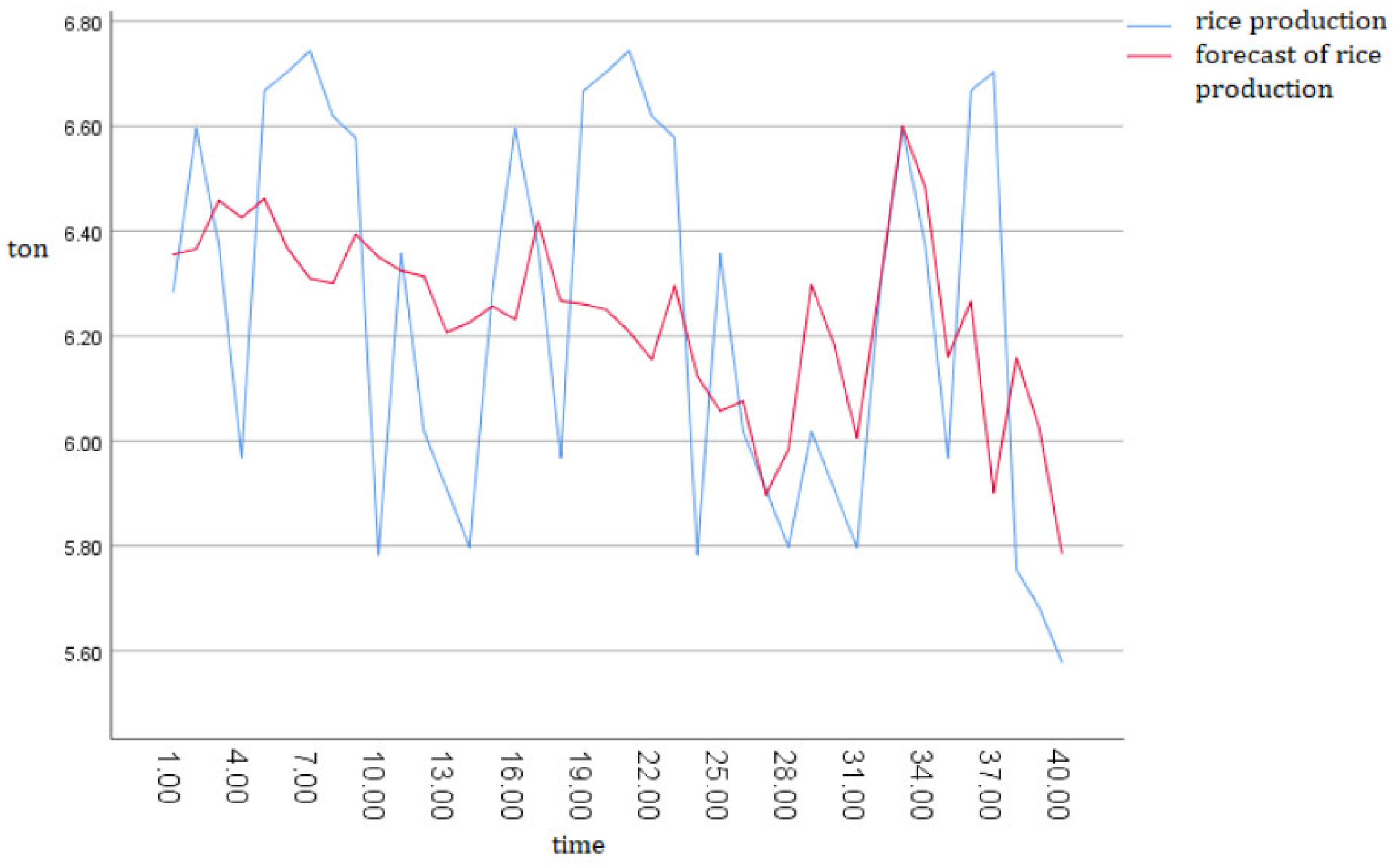
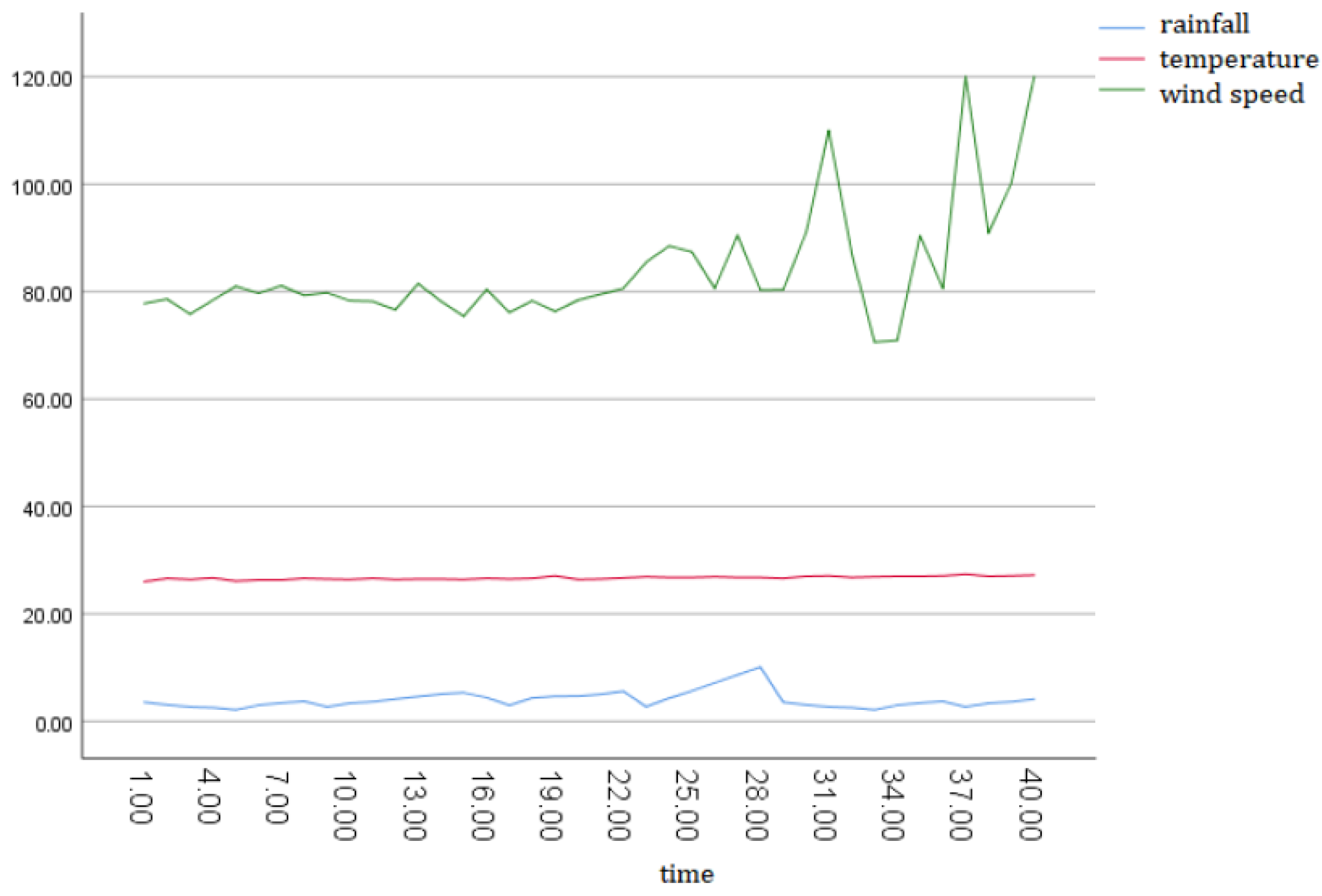
From the graph in Figure 1, it can be seen that there is a downward trend. And if we look at the graph in Figure 2, there is an increasing trend in rainfall. Meanwhile, wind speed and temperature are relatively stable. This result is in accordance with the hypothesis that if rainfall increases, rice production will decrease.

In this section, an analysis of the risks that occurred in the production process of rice farming is carried out which is caused by several factors that cause losses based on the weather index. Based on the mathematical modeling in sub-Section 4.1, weather can affect rice yields. The variable analyzed is the return on the predicted yield of rice harvest, which fluctuates with weather changes. Next, the value of VaR, CVaR, and TVaR can be determined based on the tail distribution of the exponential family. The pattern of return data is plotted and fitted using easyfit, the results of plotting the data are presented in

Table 1. Plotting results of rice yield return data.

#	Distribution	Kolmogorov Smirnov		Anderson Darling		Chi-Squared
		Statistic	Rank	Statistic	Rank	Statistic	Rank
1	Beta	0.11192	5	0.68607	4	1.75600	5
2	Exponential	0.10034	3	0.31211	1	0.61500	2
3	Exponential (2p)	0.09466	2	1.09920	5	0.82823	3
4	Gen. Extreme Value	0.10730	4	0.60817	3	1.37110	4
5	Gen. Pareto	0.08324	1	0.36822	2	0.47797	1
6	Normal	0.15392	6	1.59750	6	3.27000	6
7	Pareto	0.26462	7	6.75510	7	9.03440	7
8	Student’s t	No fit

.

From Table 1, General Pareto Distribution was the first rank, exponential distribution was the second rank, and normal distribution as justification or comparison was the sixth rank. The complete results of parameter estimation for each data distribution are presented in

Table 2. Parameter estimation results.

#	Distribution	Parameters
1	Beta	α1 = 0.50082 α2 = 1.1546 a = 9.700 × 10−4 b = 0.0659
2	Exponential	λ = 53.252
3	Exponential (2p)	λ = 56.049 γ = 9.3700 × 10−4
4	Gen. Extreme Value	k = 0.163 σ = 0.01139 μ = 0.01036
5	Gen. Pareto	k = −0.01662 σ = 0.02306 μ = −0.00105
6	Normal	σ = 0.02306 μ = −0.00105
7	Pareto	α = 0.40141 β = 9.3700 × 10−4
8	Student’s t	No fit

.

Based on the results of data processing in Table 2, the results of parameter estimation in Table 2, and the results of model development, which are presented in Theorem 1, Theorem 2, and Theorem 3, the values of risk measures at safety levels of 95%, 99%, and 99.9% were obtained and presented in Table 2.

Meanwhile, as a comparison, the exponential distribution and GPD with μ, σ, and ξ, are used, which are estimated by the principle of the moment method, with

$$E\left(X\right)=\frac{\mathsf{\sigma }}{1-\mathsf{\xi }}, \mathsf{\xi }<1 \mathrm{and} Var\left(X\right)=\frac{{\mathsf{\sigma }}^2}{{\left(1-\mathsf{\xi }\right)}^2\left(1-2\mathsf{\xi }\right) }, \mathsf{\xi }<\frac{1}{2}$$

Parameters estimated Equations (16) and (17) by moment method,

$$\begin{gathered} \mathsf{\xi }=\frac{1}{2}\left(1-\frac{{\left(E\left(X\right)-\mathsf{\mu }\right)}^2}{Var\left(X\right)}\right) \\ \mathsf{\sigma }=\left(E\left(X\right)-\mathsf{\mu }\right)\left(1-\mathsf{\xi }\right) \end{gathered}$$

If losses follow GPD, with the opportunity density function,

$$\begin{gathered} f\left(x\right)=\frac{1}{s}{\left(1+\frac{\mathsf{\xi }\left(x-\mathsf{\mu }\right)}{s}\right)}^{\left(-\frac{1}{\mathsf{\xi }}-1\right)}, \mathrm{so} \\ Va{R}_{\alpha }\left(R_{Q_t}\right)=u+\frac{\beta }{\mathsf{\xi }}\left({\left(\frac{n}{N_u}q\right)}^{-\mathsf{\xi }}-1\right), \\ TVa{R}_{\alpha }\left(R_{Q_t}\right)=\mathsf{\mu }+s\left(\frac{{\left(1-\alpha \right)}^{-\mathsf{\xi }}}{1-\mathsf{\xi }}+\frac{{\left(1-\alpha \right)}^{-\mathsf{\xi }}-1}{\mathsf{\xi }}\right),\mathsf{\xi }\ne 0 \mathrm{and} \\ TVa{R}_{\alpha }\left(R_{Q_t}\right)=\mathsf{\mu }+s\ln (1-\alpha ),\mathsf{\xi }=0 \end{gathered}$$

If the loss follows exponential, with density function

$$\begin{gathered} f\left(R_{Q_t}\right)=\lambda \exp (-\lambda R_{Q_t}) \\ TVa{R}_{\alpha }\left(R_{Q_t}\right)=\frac{-\ln (1-\alpha )+1}{\lambda } \end{gathered}$$

If the loss follows Pareto, with density function

$$\begin{gathered} f\left(R_{Q_t}\right)=\left\{\begin{array}{c}\frac{a{x}_m^a}{x^{a+1}},jikax\ge x_m\\ 0,jikax<x_m\end{array}\right. \\ TVa{R}_{\alpha }\left(R_{Q_t}\right)=\frac{x_{m}a}{{\left(1-\alpha \right)}^{\raisebox{1ex}{$1$}\!\left/ \!\raisebox{-1ex}{$\alpha $}\right.}\left(a-1\right)} \end{gathered}$$

The calculation results are presented in

Table 3. Values of VaR, CVaR, and TVaR.

Distribution	$\mathit{\alpha }$	VaR	CVaR	TVaR
Normal	0.95	0.039086	0.04114318	0.080229
	0.99	0.056688	0.05726110	0.113950
	0.999	0.075548	0.07562391	0.151172
Exponential	0.95	0.0231298	0.02345126	0.04658106
	0.99	0.0324114	0.05453217	0.08694357
	0.999	0.0567435	0.06675345	0.12349695
GPD	0.95	0.0290863	0.03113418	0.06022048
	0.99	0.0478682	0.05834212	0.10621032
	0.999	0.0643547	0.06564287	0.12999757

.

Based on Table 3, the results of the data analysis, some comments can be given. The results of fitting the data with a normal distribution approach produce VaR values that increase with increasing $\mathsf{\alpha }$, as well as CVaR and TVaR values. The largest VaR value occurs in the normal distribution model approach, while the smallest VaR value occurs in the General Pareto distribution approach. Meanwhile, in the exponential distribution approach, the VaR and TVaR values are relatively stable. These results are in line with the results of data fitting, which are presented in Table 1, where the order of data fit starts from the exponential distribution, General Pareto distribution, and normal distribution. This is also equivalent to the results obtained [1,5,20,24].

The possible losses that can be suffered by farmers can be calculated by referring to the size of the risk of loss and the amount of capital invested. If referring to the average production cost per hectare per planting period, that farmers currently spend is IDR 8,000,000.00 and an average production of IDR 13,000,000.00, then the net profit is around IDR 5,000,000,000.00. The possible loss of production capital is presented in Table 3. This result is obtained if it is assumed that the fixed capital for the rice production process per hectare per planting period is IDR 8,000,000.00, then the potential loss that may occur in the capital is presented in

Table 4. Value of risk of loss on capital (IDR).

Distribution	$\mathit{\alpha }$	VaR	CVaR	TVaR
Normal	0.95	312,688.00	329,145.44	641,832.00
	0.99	453,504.00	458,088.80	911,600.00
	0.999	604,384.00	604,991.28	1,209,376.00
Exponential	0.95	185,038.40	187,610.08	372,648.48
	0.99	259,291.20	436,257.36	695,548.56
	0.999	453,948.00	534,027.60	987,975.60
GPD	0.95	232,690.40	249,073.44	481,763.84
	0.99	382,945.60	466,736.96	849,682.56
	0.999	514,837.60	525,142.96	1,039,980.56

.

The amounts of losses suffered by farmers will depend on when the planting period, which of course will determine when the harvest period. Based on Table 3, the biggest possible loss will occur around October, when the harvest will take place around the end of January-early February. Meanwhile, minimal losses occur in March–April with the harvest period around July-August. The results of the complete calculation of losses are presented in Table 4. These results illustrate the magnitude of losses that may be experienced by farmers. They will be used as the basis for the calculation model or the estimated premium price.

Rahmawati [44] states that the phenomenon of climate change is an erratic weather condition. This study observes the technical efficiency of rice farming including the factors that influence it in uncertain weather conditions. The production function model is used by the Cobb–Douglas translog frontier to analyze the factors that affect rice production and technical efficiency. The results of the production function show that the factors that affect rice production are land, labor, organic fertilizer, N fertilizer, irrigation, pollution, season, and location. Rice farming has not been efficient. The results of this study imply that rice farming efficiency for sustainable agriculture needs to use optimal inputs, encourage farmers’ skills, and develop irrigation infrastructure. However, this study did not discuss the effect of weather on the risk of paddy yields.

The results of our study are in accordance with the results obtained from the study [40]. Sukono [40] stated that the agricultural sector is directly affected by climate variables. The existence of climate variability causes considerable risk to agricultural productivity. Thus, risk management is an alternative to reducing risk, including optimizing the allocation of agricultural land and selecting crop insurance for certain planting dates. This paper investigates several possible considerations of rice farming losses based on weather changes. We conclude that the weather index insurance policy is the best option that farmers can choose for each planting date, the higher the significance value considered, the greater the Value at Risk, Conditional Value at Risk, and Tail Value at Risk.

5. Discussion

Agricultural activity is changing in pattern currently caused by erratic weather conditions. Weather changes have made us aware of the importance of studying extreme events, which is the main step in mitigating the risk of crop loss. The main strategic steps are detecting potential risks, collecting data on risk, and tracking losses that have occurred. After that, the mitigation process is carried out by determining the amount of risk as an expectation of losses.

In this study, modeling is carried out to estimate the risk of rice yield loss. The rice yield was modeled using the Cobb–Douglas model. The forecast production results are modified into the return production results. From the return modeling results, there are modeled the VaR, CVaR, and TVaR values as a measure of the risk of loss. These results are written in Theorem 1, Theorem 2, and Theorem 3.

From those models, we verified the results through data analysis. The data used are presented in Appendix D. Based on the hypothesis, we can find that the data on rainfall, wind speed, and high temperature will cause a decrease in the amount of production, as shown in Figure 1 and Figure 2. From the two figures, it can be seen that, especially if the rainfall increases, the amount of production decreases. A decrease in the amount of production will cause a risk of loss. The risk of this loss can be measured using a risk measure. From the results of the discussion, we concentrate on the problem of estimating the risk of agricultural financial losses using the VaR, CVaR, and TVaR measures, which are the most classic risk indicators used by financial institutions as carried out by [46,47,48,49].

The results of the modeling, shown in Theorem 1, Theorem 2, and Theorem 3 and proven in Appendix A, Appendix B and Appendix C, with the results of data analysis, are not contradictory. This result is a refinement of the research conducted by Sukono et al. [40]. From the results of this research, we can see that the risk measurement using VaR does not consider all possible worst cases. The slightest of the worst cannot be ignored.

The estimated risk for this study was measured by calculating the values of VaR, CVaR, and TVaR. The results can be seen in Table 3. While the value of losses that occurred can be seen in Table 4. These results were measured parametrically using the data distribution fitted with easyfit. The distribution used is selected based on the ranking of the data fitting results. From Table 1, General Pareto distribution, exponential, and normal are selected. Even though the normal distribution is in the sixth rank, it is chosen as the counterpart to the other two distributions selected.

Furthermore, it is necessary to consider the maximum potential loss as a precaution in making decisions. The results in Table 4 can be considered in determining the next steps for the formulation of loss risk management. From these three distributions, the estimation results in the greatest potential loss occurred if the losses are normally distributed.

One of the benefits of this study is that it can help insurance companies to take policies and develop types of agricultural insurance products. This will help ensure that the insurer can determine the premium price correctly for protection against losses due to weather changes. On the other hand, this can be a consideration for farmers, especially in Bandung Regency in making decisions on whether to insure their rice crops or not. This is certainly very helpful for farmers in making decisions.

6. Conclusions

Based on the results of the discussion, it can be concluded that weather factors have an important role in considering the risk of loss in rice farming. From the results of this modeling, an increase in the intensity of the weather, especially rainfall will result in a reduced return of rice production. The results of the analysis show that the potential for losses varies depending on the distribution pattern of the extreme data. If you look at the results in Table 2, then the estimated loss using the Generalized Pareto Distribution is the best decision. However, if we rely on the return of crop yields, then the normal distribution will provide results that are more careful in measuring the risk of loss.

The analysis results of this study are in accordance with the characteristics of the risk of loss so that the result of the maximum potential loss becomes a reference for mitigating the risks that may occur. If the risk of this loss is borne by the agricultural insurance company, not by the farmer, the insurance company needs to provide reserve funds that can cover the potential loss. If the reserve fund cannot be provided, it is feared that there will be disturbances in the rice production process. In particular, extreme unforeseen events such as extreme weather, hurricanes, and floods can occur at any time. If this happens and the reserve funds are unprepared, it can certainly make the insurance company collapse. Therefore, the maximum potential loss is an important concern in risk mitigation efforts.

This research still has limitations related to the exploration of loss risk data and weather data. Therefore, further research can explore the risk of loss and estimate the loss to be better, so it can make risk management safer.

References

- Riaman, R.; Sukono, S.; Supian, S.; Ismail, N. Analysing the decision making for agricultural risk assessment: An application of extreme value theory. Decis. Sci. Lett. 2021, 10, 351–360. [Google Scholar] [CrossRef]
- Raghu, S.; Guru-Pirasanna, G.; Baite, M.S.; Yadav, M.K.; Prabhukarthikeyan, S.R.; Keerthana, U.; Rath, P.C. Estimation of yield loss and relationship of weather parameters on incidence of bakanae disease in paddy varieties under shallow low land ecologies of Eastern India. J. Environ. Biol. 2021, 42, 995–1001. [Google Scholar] [CrossRef]
- Ali, S.; Ghosh, B.C.; Osmani, A.G.; Hossain, E.; Fogarassy, C. Farmers’ climate change adaptation strategies for reducing the risk of rice production: Evidence from rajshahi district in Bangladesh. Agronomy 2021, 11, 600. [Google Scholar] [CrossRef]
- Brahmantyo, Y.; Riaman, R.; Sukono, F. Willingness to Pay of Fishermen Insurance Using Logistic Regression with Parameter Estimated by Maximum Likelihood Estimation Based on Newton Raphson Iteration. J. Mat. Integr. 2021, 17, 15–21. [Google Scholar] [CrossRef]
- Riaman, R.; Sukono, S.; Supian, S.; Ismail, N. Determining the premium of paddy insurance using the extreme value theory method and the operational value at risk approach. J. Phys. Conf. Ser. 2021, 1722, 012059. [Google Scholar] [CrossRef]
- Sang, A.J.; Tay, K.M.; Lim, C.P.; Nahavandi, S. Application of a Genetic-Fuzzy FMEA to Rainfed Lowland Paddy Production in Sarawak: Environmental, Health, and Safety Perspectives. IEEE Access 2018, 6, 74628–74647. [Google Scholar] [CrossRef]
- Sujarwo, S.; Rukmi, S.M.N. Factors affecting agricultural insurance acceptability of paddy farmers in East Java, Indonesia. J. Manaj. Agribisnis 2018, 15, 143. [Google Scholar] [CrossRef]
- Savary, S.; Horgan, F.; Willocquet, L.; Heong, K.L. A review of principles for sustainable pest management in paddy. Crop. Prot. 2012, 32, 54–63. [Google Scholar] [CrossRef]
- Sheehy, J.E.; Mitchell, P.L.; Ferrer, A.B. Decline in paddy grain yields with temperature: Models and correlations can give different estimates. Field Crops Res. 2006, 98, 151–156. [Google Scholar] [CrossRef]
- Dhaene, J.; Kukush, A.; Linders, D.; Tang, Q. Remarks on quantiles and distortion risk measures. Eur. Actuar. J. 2012, 2, 319–328. [Google Scholar] [CrossRef]
- Tavanaie Marvi, M.; Linders, D. Decomposition of Natural Catastrophe Risks: Insurability Using Parametric CAT Bonds. Risks 2021, 9, 215. [Google Scholar] [CrossRef]
- Chen, Q.; Zhang, J.; Zhang, L. Risk assessment, partition and economic loss estimation of paddy production in China. Sustainability 2015, 7, 563–583. [Google Scholar] [CrossRef]
- Liu, F.; Corcoran, C.P.; Tao, J.; Cheng, J. Risk perception, insurance recognition and agricultural insurance behavior—An empirical based on dynamic panel data in 31 provinces of China. Int. J. Disaster Risk Reduct. 2016, 20, 19–25. [Google Scholar] [CrossRef]
- Ramaswami, B. Supply response to agricultural insurance: Risk reduction and moral hazard effects. Am. J. Agric. Econ. 1993, 75, 914–925. [Google Scholar] [CrossRef]
- Polukhin, A.A.; Panarina, V.I. Financial Risk Management for Sustainable Agricultural Development Based on Corporate Social Responsibility in the Interests of Food Security. Risks 2022, 10, 17. [Google Scholar] [CrossRef]
- Kijima, Y. Farmers’ risk preferences and paddy production: Experimental and panel data evidence from Uganda. PLoS ONE 2019, 14, 219202. [Google Scholar]
- Budhathoki, N.K.; Lassa, J.A.; Pun, S.; Zander, K.K. Farmers’ interest and willingness-to-pay for index-based crop insurance in the lowlands of Nepal. Land Use Policy 2019, 85, 1–10. [Google Scholar] [CrossRef]
- Ghoshal, P.; Goswami, B. Cobb-Douglas production function for measuring efficiency in Indian agriculture: A region-wise analysis. Econ. Aff. 2017, 62, 295084. [Google Scholar] [CrossRef]
- Kumar, A.J.; Rohila, A.K.; Pal, V.K. Profitability and resource use efficiency in vegetable cultivation in Haryana: Application of Cobb-Douglas production model. Indian J. Agric. Sci. 2018, 88, 153–157. [Google Scholar]
- Wang, Y.; Huang, J.; Wang, J.; Findlay, C. Mitigating paddy production risks from drought through improving irrigation infrastructure and management in China. Aust. J. Agric. Resour. Econ. 2018, 62, 161–176. [Google Scholar] [CrossRef]
- Wang, H.H.; Tack, J.B.; Coble, K.H. Frontier studies in agricultural insurance. Geneva Pap. Risk Insur.-Issues Pract. 2020, 45, 1–4. [Google Scholar] [CrossRef]
- Yanuarti, R.; Aji, J.M.M.; Rondhi, M. Risk aversion level influence on farmer’s decision to participate in crop insurance: A review. Agric. Econ. 2019, 65, 481–489. [Google Scholar] [CrossRef]
- Villano, R.; Fleming, E. Technical inefficiency and production risk in paddy farming: Evidence from Central Luzon Philippines. Asian Econ. J. 2006, 20, 29–46. [Google Scholar] [CrossRef]
- Vedenov, D.V.; Sanchez, L. Weather derivatives as risk management tool in Ecuador: A case study of paddy production. In Proceedings of the Selected Paper Prepared for Presentation at the Southern Agricultural Economics Association Annual Meeting, Corpus Christi, TX, USA, 5–8 February 2011. [Google Scholar]
- Khai, H.V.; Yabe, M. Technical efficiency analysis of paddy production in Vietnam. J. ISSAAS 2011, 17, 135–146. [Google Scholar]
- Nantui, M.F.; Bruce, S.D.; Yaw, O.A. Adaptive capacities of farmers to climate change adaptation strategies and their effects on paddy production in the northern region of Ghana. Russ. J. Agric. Socio-Econ. Sci. 2012, 11, 9–17. [Google Scholar]
- Nikkhah, A.; Emadi, B.; Soltanali, H.; Firouzi, S.; Rosentrater, K.A.; Allahyari, M.S. Integration of life cycle assessment and Cobb-Douglas modeling for the environmental assessment of kiwifruit in Iran. J. Clean. Prod. 2016, 137, 843–849. [Google Scholar] [CrossRef]
- Ioan, C.A.; Ioan, G. The Complete Theory of Cobb-Douglas Production Function. Acta Univ. Danub. 2015, 11, 74–114. [Google Scholar]
- Kaka, Y.; Shamsudin, M.N.; Radam, A.; Abd Latif, I. Profit efficiency among paddy farmers: A Cobb-Douglas stochastic frontier production function analysis. J. Asian Sci. Res. 2016, 6, 66–75. [Google Scholar] [CrossRef]
- Umar, H.S.; Girei, A.A.; Yakubu, D. Comparison of Cobb-Douglas and Translog frontier models in the analysis of technical efficiency in dry season tomato production. Agrosearch 2017, 17, 67. [Google Scholar] [CrossRef]
- Singh, A.K.; Narayanan, K.G.; Sharma, P. Effect of climatic factors on cash crop farming in India: An application of Cobb-Douglas production function model. Int. J. Agric. Resour. Gov. Ecol. 2017, 13, 175–210. [Google Scholar] [CrossRef]
- Kumar, V.; Singh, S.; Kumar, R.M.; Sharma, S.; Tripathi, R.; Nayak, A.K.; Ladha, J.K. Growing Paddy in Eastern India: New Paradigms of risk reduction and improving productivity. In The Future Paddy Strategy for India; Academic Press: New Delhi, India, 2017; pp. 221–258. [Google Scholar]
- Entezari, A.F.; Wong, K.S.; Ali, F. Malaysia’s Agricultural Production Dropped and the Impact of Climate Change: Applying and Extending the Theory of Cobb Douglas Production. Agrar. J. Agribus. Rural. Dev. Res. 2021, 7, 127–141. [Google Scholar] [CrossRef]
- Uche, C.O.; Umar, H.S.; Girei, A.A.; Ibrahim, H.Y. Performance of Translog and Cobb-Douglas models in the estimation of technical efficiency of Irish potato production in Plateau State, Nigeria. Agro-Sci. 2021, 20, 62–67. [Google Scholar] [CrossRef]
- Kaylen, M.S.; Loehman, E.T.; Preckel, P.V. Farm-level analysis of agricultural insurance: A mathematical programming approach. Agric. Syst. 1989, 30, 235–244. [Google Scholar] [CrossRef]
- Riaman, R.; Sukono, S.; Supian, S.; Ismail, N. Mapping in the Topic of Mathematical Model in Paddy Agricultural Insurance Based on Bibliometric Analysis: A Systematic Review Approach. Computation 2022, 10, 50. [Google Scholar] [CrossRef]
- Yamuangmorn, S.; Jumrus, S.; Jamjod, S.; Yimyam, N.; Prom-u-Thai, C. Stabilizing grain yield and nutrition quality in purple paddy varieties by management of planting elevation and storage conditions. Agronomy 2021, 11, 83. [Google Scholar] [CrossRef]
- Islam, M.M.; Ahamed, T.; Noguchi, R. Land suitability and insurance premiums: A GIS-based multicriteria analysis approach for sustainable paddy production. Sustainability 2018, 10, 1759. [Google Scholar] [CrossRef]
- Zulkafli, Z.; Muharam, F.M.; Raffar, N.; Jajarmizadeh, A.; Abdi, M.J.; Rehan, B.M.; Nurulhuda, K. Contrasting Influences of Seasonal and IntraSeasonal Hydroclimatic Variabilities on the Irrigated Paddy Paddies of Northern Peninsular Malaysia for Weather Index Insurance Design. Sustainability 2021, 13, 5207. [Google Scholar] [CrossRef]
- Sukono, S.; Riaman, R.; Supian, S.; Hidayat, Y.; Saputra, J.; Pribadi, D. Investigating the agricultural losses due to climate variability: An application of conditional value-at-risk approach. Decis. Sci. Lett. 2021, 10, 71–78. [Google Scholar] [CrossRef]
- Tsakaev, A.K.; Saidov, Z.A. Identification and analysis of the risk of reducing the stability of the Russian agricultural insurance system. Espacios 2018, 39, 22090. [Google Scholar]
- Varadan, R.J.; Kumar, P. Impact of crop insurance on paddy farming in Tamil Nadu. Agric. Econ. Res. Rev. 2012, 25, 291–298. [Google Scholar]
- Diop, A.N. Agricultural Risk Pricing in Senegal. J. Math. Financ. 2019, 9, 182. [Google Scholar] [CrossRef]
- Rahmawati, N.; Isnawan, B.H. Technical efficiency of paddy farm under risk of uncertainty weather in Yogyakarta, Indonesia. IOP Conf. Ser. Earth Environ. Sci. 2020, 423, 012036. [Google Scholar]
- Asimit, A.V.; Vernic, R.; Zitikis, R. Evaluating risk measures and capital allocations based on multi-losses driven by a heavy-tailed background risk: The multivariate Pareto-II model. Risks 2013, 1, 14–33. [Google Scholar] [CrossRef]
- Amnuaylojaroen, T.; Chanvichit, P.; Janta, R.; Surapipith, V. Projection of paddy and maize productions in Northern Thailand under climate change scenario RCP8. 5. Agriculture 2021, 11, 23. [Google Scholar] [CrossRef]
- Faroni, S.; Le Courtois, O.; Ostaszewski, K. Equivalent Risk Indicators: VaR, TCE, and Beyond. Risks 2022, 10, 142. [Google Scholar] [CrossRef]
- Syuhada, K.; Neswan, O.; Josaphat, B.P. Estimating Copula-Based Extension of Tail Value-at-Risk and Its Application in Insurance Claim. Risks 2022, 10, 113. [Google Scholar] [CrossRef]
- Demirer, R.; Gkillas, K.; Kountzakis, C.; Mavragani, A. Risk Appetite and Jumps in Realized Correlation. Mathematics 2020, 8, 2255. [Google Scholar] [CrossRef]
Figure 1.
Trends in rice productivity in West Java area.
Figure 2.
Weather Data in Bandung Regency, West Java.