DC Drive Adaptive Speed Controller Based on Hyperstability Theory

Abstract

The scope of this research is to develop a hyperstable adaptive control system of a direct current (DC) drive speed for effective load torque attenuation. The proposed speed controller is based on the model reference adaptive control framework and integrated into the conventional DC drive cascade control system. Its main features are as follows: (1) the boundedness of the control action signal, as well as the armature current control loop non-stationarities, are taken into consideration with the help of the reference model hedging technique; (2) its inputs include only measurable signals, thus there is no need to use any kind of state estimators; (3) it attenuates the disturbances, which are matched with its control action signal, particularly, the inertia moment non-stationarity and load torque. The asymptotic hyperstability of the obtained DC drive control system is proven with the help of Lyapunov’s theorems and Popov’s criterion. The numerical experiments corroborate the obtained results. They include the demonstration of disadvantages of the conventional cascade control system under conditions of the drive parameters’ non-stationarity and advantages of the proposed solution for different disturbance types and amplitudes.

1. Introduction

Nowadays, electric motors are the main actuators, which are applied to control technological processes of various branches of industry [1]. Owing to the simplicity of their control, the direct current (DC) motors with separate excitation of the armature and rotor windings are the most widespread among all electric motors. However, due to the structural features, such motors are energy inefficient and require periodic maintenance of the collector-and-brush assembly unit. Therefore, in recent decades, because of the power electronics development, there is a tendency in the industry to replace DC motors with asynchronous and synchronous ones, which do not have the above-mentioned disadvantages. However, under conditions of real production, such replacement, as a rule, requires significant capital investments for the renewal of the electric motors and accompanying control electronic and computer equipment (replacement of the thyristor converters with frequency converters, etc.). Today, many enterprises are not ready to make such capital investments, and therefore, the most promising solution is to find ways to improve the energy and economic efficiency of DC motors.

There is an opinion [2], that it is possible to increase the DC motors efficiency indirectly, i.e., by means of control quality improvement of the technological processes, in which such motors are used as the actuating mechanisms. The main factor, which has an impact on such quality, is the deterioration of the motor speed and/or rotor position control, which are/is caused by the non-stationarity of such motor characteristics. In turn, this instability is usually caused by changes of values of such parameters as the motor inertia moment and the load torque. For example, according to expert opinion [3], a factor of the inertia moment variation of such units as coilers and industrial robots can reach 2–10 times compared to its nominal value. At the same time, the factor of the load torque variation of such units as rolling mills reaches 2–3 times compared to its nominal value. In this regard, the problem of the DC motor non-stationarity compensation to improve its speed control quality is actual.

To date, the speed control of the DC motors is usually implemented as a cascade control system [1,3] based on a proportional-integral (PI) controller with stationary values of the parameters of its proportional and integral parts. Such parameters are calculated to make the speed loop follow the symmetrical optimum requirements [1,4]. Accordingly, to compensate for the influence of the non-stationarity of the motor, it is necessary either to provide such a PI-controller with the adaptive properties by its parameters adjustment or to develop a new adaptive speed controller.

Let us consider the main methods related to both mentioned solutions, as the computational power of the modern industrial programmable logic controllers (PLCs) and micro-controller devices is high enough for the practical implementation of such more complex, but also more efficient control systems. This means that, from the point of view of software and technical implementation, there are no obstacles to solving the above-stated problem.

In [5,6], the neural network and fuzzy tuners of the speed PI-controller parameters are proposed, respectively. The advantages of these tuners include the rules of the PI-controller parameters adjustment, which are understandable by the process automation engineers. As for their disadvantages, the main of them is the open question of such closed-loop control systems stability. In [7], based on the feedback linearization and the second Lyapunov methods, an adaptive speed controller is developed, which has another structure that is different from the PI one. The disadvantage of this controller is the necessity to know some values, which are immeasurable in practice, as well as the facts that: (1) it does not include an algorithm to compensate for the load torque and (2) the boundedness of the control action signal is not taken into consideration. In [8], according to the model reference adaptive control (MRAC) method, a tuner of the speed PI-controller parameters is proposed, which takes into account the control signal boundedness. But it, as well as in [7], is based on the practically immeasurable values and provides only the robustness of the closed-loop control system to the load torque, but not its compensation.

This paper is to take all the shortcomings of the methods from [5,6,7,8] into consideration and propose an adaptive DC motor speed control system, which: (1) uses only measurable signals; (2) considers the boundedness of the control signal; and (3) adaptively compensates for the load torque.

To develop such a system, the results of [8], the method of the adaptive laws synthesis based on the hyperstability criterion [9], and the notion of strictly positive real transfer functions [10], which have been successfully applied to control composite [11] and non-square systems [12], are used. Considering the known method of the reference model hedging to adapt to the boundedness of the control signal [13], the approach to hedge the reference model to take into account the bounded input–bounded output (BIBO) stable unmodeled dynamics of the plant will be proposed and then applied in this research.

The study is organized as follows. Section 2 contains a problem statement and the main result. Section 3 is to demonstrate the results of the numerical experiments. The study is wrapped-up with the concluding remarks. The proof of the proposed theorem is in the Appendix A.

2. Problem Statement and Methods

2.1. Disadvantages of Conventional Cascade DC Drive Control System

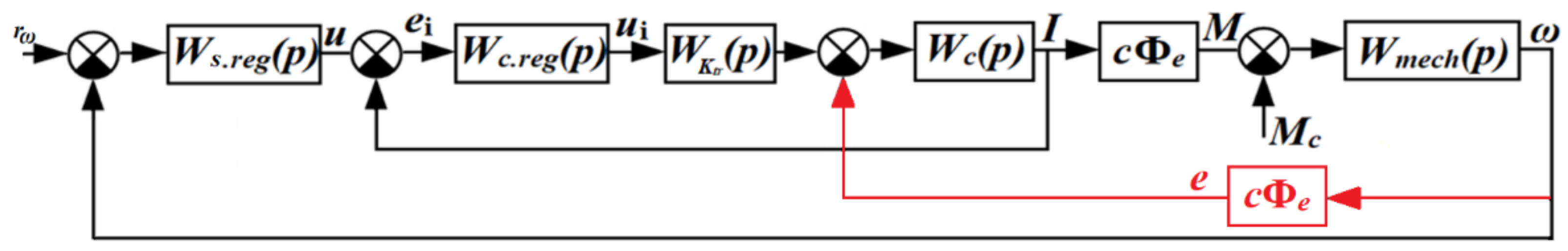
The conventional cascade DC drive control system is shown in Figure 1.

Here, $c$ is the torque constant; ${\Phi }_e$ is the magnetic flux; $I$ is the armature current; $\mathsf{\omega }$ is the rotor speed; $u$ is the control action signal (output of the speed controller) and a setpoint value for the armature current loop $\left(u_{min}\le u\le u_{max}\right)$; $M_c$ is the load torque; and $M$ is the motor electrodynamic torque. $W_{mech}\left(p\right)$ is a transfer function of the drive mechanics $\left(p:=\frac{d}{dt}\right)$, $W_c\left(p\right)$ is a transfer function of the armature winding, $e_i$ is an armature current control error, $e$ is a back electromotive force (back-EMF), $W_{c.reg}\left(p\right)$ is an armature current controller, $W_{s.reg}\left(p\right)$ is a speed controller, $u_i$ is the armature current controller output $\left(u_{i\hspace{0.33em}min}\le u_i\le u_{i\hspace{0.33em}max}\right)$, $W_{K_{tr}}\left(p\right)$ is a thyristor converter transfer function, and $r_{\mathsf{\omega }}$ is a speed setpoint. The transfer functions $W_{mech}\left(p\right),\hspace{0.33em}{W}_c\left(p\right),\hspace{0.33em}{W}_{K_{tr}}\left(p\right)$ are shown below:

$$W_{mech}\left(p\right)=\frac{1}{J_{\Sigma }p},\hspace{0.33em}\hspace{0.33em}\hspace{0.33em}\hspace{0.33em}{W}_c\left(p\right)=\frac{\frac{1}{R}}{\frac{L}{R}p+1},\hspace{0.33em}\hspace{0.33em}\hspace{0.33em}\hspace{0.33em}{W}_{K_{tr}}\left(p\right)=\frac{K_{tr}}{T_{\mathsf{\mu }}p+1},$$

(1)

where $J_{\Sigma }$ is the inertia moment of a motor shaft, $R$ is an armature resistance, $T_{\mathsf{\mu }}$ is the thyristor converter time constant, $K_{tr}$ is a thyristor converter gain, and $L$ is an armature inductance. The transfer functions of the controllers will be defined below.

Certainly, this control scheme has a lot of advantages, because of which it is broadly used in practice: (1) the fact that the physical limits on the values of the motor armature current and voltage are taken into account; (2) the scheme provides the astatism of the first order for the speed control loop when its controller parameters are calculated in accordance with the symmetrical optimum; and (3) there is no need to know the derivatives of the measured output variables (speed and armature current) to calculate the control action. The armature current controller in this scheme is usually calculated using the technical (modulus) optimum requirements (step response with 4.3% overshoot and phase margin 63⁰) and structurally implemented as a PI-controller:

$$W_{c.reg}\left(p\right)=\frac{L}{a_I{T}_{\mathsf{\mu }}{K}_{tr}}+\frac{R}{a_I{T}_{\mathsf{\mu }}{K}_{tr}p}.$$

(2)

Here $a_I$ = 2 is the conventional parameter used to meet the modulus optimum requirements.

The speed controller in such a scheme usually follows the modulus or symmetrical optimum requirements and is chosen as a proportional (P) or PI controller, respectively. Typically, considering speed, automatic electric drive systems are required to provide zero steady-state error, thus the symmetrical optimum (step response with 43% overshoot and phase margin 37⁰) is applied more often. In such a case, the speed PI-controller is defined as:

$$W_{s.reg}\left(p\right)=\frac{J_{\Sigma }}{a_I^2{T}_{\mathsf{\mu }}^{}c{\Phi }_e}+\frac{J_{\Sigma }}{a_{\mathsf{\omega }}{a}_I^3{T}_{\mathsf{\mu }}^{2}c{\Phi }_{e}p}.$$

(3)

Here $a_{\mathsf{\omega }}$ = 4 is the conventional parameter used to meet the symmetrical optimum requirements.

In the general case, the structural scheme parameters $M_c$, $J_{\Sigma }$, and $c{\Phi }_e$ are considered to be a priori unknown values.

From Equations (2) and (3), it follows that the parameters of the controllers of the electric drive depend on the values of its electrical and mechanical parameters. In particular, the armature current PI controller depends on the parameters of the electric circuits of the motor and the low-value uncompensated time constant $T_{\mathsf{\mu }}$. The speed PI controller depends on the parameters of the motor mechanics and $T_{\mathsf{\mu }}$ as well. As it is mentioned in the Introduction section, considering real electric drives, in the course of their normal functioning, the change of the motor electric circuits parameters (in particular, the armature resistance $R$) may reach up to 50% of the nominal values. At the same time, the motor mechanics parameters (the inertia moment) may change in a step-like way or as smooth functions of time. This is defined by the types of mechanical gears of a certain mechanism to be controlled. The most significant changes of the inertia moment occur in such mechanisms as winding machines used in the metallurgical and pulp and paper industries and excavators in the mining industry, as well as in transport mechanisms and manipulators. Considering such non-stationarity of the mechanics and electric circuits of the electric drive, the speed control quality may differ significantly from the required one. This will be demonstrated in the third section of this study.

2.2. Problem Statement

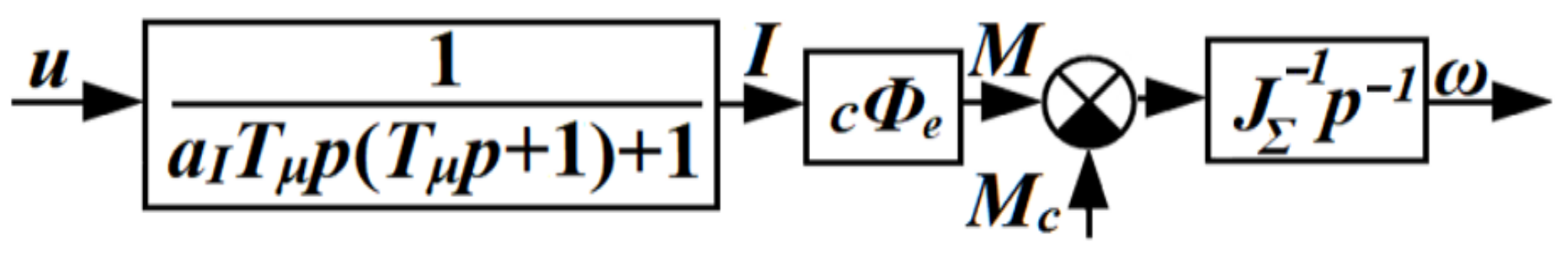
The general structural scheme of the plant of the separately excited DC motor speed control loop is shown in Figure 2 [1]. The transfer function to transform $u$ into $I$ is obtained as a closed-loop transfer function:

$$W_{c.reg}\left(p\right)W_{K_{tr}}\left(p\right)W_c\left(p\right)/\left(1+W_{c.reg}\left(p\right)W_{K_{tr}}\left(p\right)W_c\left(p\right)\right).$$

The scheme in Figure 2 is relevant when the armature current loop is tuned to follow the modulus optimum ($a_I$ = 2), and the back-EMF is compensated (red lines in Figure 1 do not exist). The following assumption is introduced for further analysis.

Assumption 1.

The load torque M_c is matched with the control action signal$u$.

The scheme in Figure 2 can be transformed into the one shown in Figure 3 as:

$$\begin{array}{c}\frac{1}{a_I{T}_{\mathsf{\mu }}p\left(T_{\mathsf{\mu }}p+1\right)+1}=1+\frac{-a_I{T}_{\mathsf{\mu }}p\left(T_{\mathsf{\mu }}p+1\right)}{a_I{T}_{\mathsf{\mu }}p\left(T_{\mathsf{\mu }}p+1\right)+1},\\ \underset{M}{\underbrace{Ic{\Phi }_e}}-M_c=\left(I-\frac{M_c}{c{\Phi }_e}\right)c{\Phi }_e.\end{array}$$

Considering Assumption 1, the plant of the DC drive speed control loop is described in the extended state space as:

$$\begin{array}{c}\dot{x}=Ax+B\left(u+\Delta \left(u\right)-{\mathsf{\tau }}_e\right)\\ x=\left[\begin{array}{c}\mathsf{\theta }\\ \mathsf{\omega }\end{array}\right]; A=\left[\begin{array}{cc}0& 1\\ 0& 0\end{array}\right]; B=\left[\begin{array}{c}0\\ b\end{array}\right]; b=c{\Phi }_e{J}_{\Sigma }^{-1}; {\mathsf{\tau }}_e=\frac{1}{c{\Phi }_e}{M}_c,\end{array}$$

(4)

where $x$ ∈ R² is the state vector; ${\mathsf{\tau }}_e$ is the disturbance, which is caused by the load torque $M_c$ and matched with the control action signal; $\Delta \left(u\right)$ is a function to describe unmodeled dynamics (the disturbance, which is caused by the armature current loop dynamics and could not be compensated by the control signal $u$), $A$ ∈ R^2×2 is the state matrix, and $B$ ∈ R^2×1 is the input matrix. The pair $\left(A,B\right)$ is controllable. The following assumption is introduced about the disturbance, $\Delta \left(u\right)$.

Assumption 2.

The disturbance $\Delta \left(u\right)$, which could not be compensated by the control signal $u$, is bounded $\Delta \left(u\right)\in L_{\infty }$ if the control action signal $u$ is bounded $u\in L_{\infty }$.

Then, it is rational to choose the control law $u$ for the system (4) as an adaptive PI-controller with saturations:

$$u=sat\left({\widehat{K}}_I{\displaystyle \underset{0}{\overset{t}{\int }}sa{t}_I\left(e\right)d\mathsf{\tau }}+{\widehat{K}}_{P}e+{\widehat{u}}_{ad}\right).$$

(5)

Here, ${\widehat{K}}_P$ is the parameter of the PI-controller proportional part; ${\widehat{K}}_I$ is the parameter of the PI-controller integral part, ${\widehat{u}}_{ad}$ is an additional term to compensate for ${\mathsf{\tau }}_e$; $e=r_{\mathsf{\omega }}-\mathsf{\omega }$ is the tracking error, i.e., the difference between the rotor speed setpoint $r_{\mathsf{\omega }}$ and its actual value. The fact that $u$ (the armature current) is bounded is taken into consideration in (5) with the help of the saturation function $sat\left(.\right)$ and the Anti-Windup procedure $sa{t}_I\left(.\right)$:

$$\begin{array}{c}sat\left(v_{sat}\right)=\left\{\begin{array}{l}{u}_{max} \mathrm{if} v_{sat}\ge u_{max}\\ v_{sat} \mathrm{if} u_{min}<v_{sat}<u_{max}\\ u_{min} \mathrm{if} v_{sat}\le u_{min}\end{array}\right., \\ sa{t}_I\left(e\right)=\left\{\begin{array}{l}0 \mathrm{if} \left[v_{sat}\ge u_{max}\vee v_{sat}\le u_{min}\right]\wedge \left[e>0\vee e<0\right]\\ e \mathrm{otherwise}\end{array}\right..\end{array}$$

(6)

where $v_{sat}$ is the control action $u$ value after application of the Anti-Windup procedure $sa{t}_I\left(.\right)$, which is used in the integral part of the controller.

Remark 1.

It follows from the chosen control law (5) with the Anti-Windup procedure (6) that Assumption 2 is met for (5).

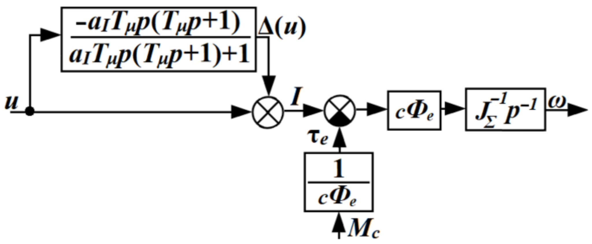
Remark 2.

In accordance with Figure 3, the disturbance $\Delta \left(u\right)$ is generated as a BIBO transfer function:

$$W_1\left(p\right)=\frac{-a_I{T}_{\mathsf{\mu }}p\left(T_{\mathsf{\mu }}p+1\right)}{a_I{T}_{\mathsf{\mu }}p\left(T_{\mathsf{\mu }}p+1\right)+1}$$

(7)

only if the following holds simultaneously for the motor armature current control loop: (1) the armature current controller is tuned to follow the modulus optimum requirements; (2) the back-EMF is fully compensated (we consider the scheme in Figure 1, but without red lines); (3) the motor armature current controller output is not saturated.

Otherwise, the disturbance is generated by some BIBO transfer function$W_2\left(p\right)$of higher order compared to (7), but the requirements of Assumption 2 are still met.

Using (5), let the notion of the control law $v$, which is formed without (6), be introduced:

$$\begin{array}{c}v=\widehat{K}\left(r-y\right)+{\widehat{u}}_{ad},\\ \widehat{K}=\left[{\widehat{K}}_I\hspace{0.33em}\hspace{0.33em}\hspace{0.33em}{\widehat{K}}_P\right], \mathrm{r}={\left[{\displaystyle \underset{0}{\overset{t}{\int }}{r}_{\mathsf{\omega }}d\mathsf{\tau }}\hspace{0.33em}\hspace{0.33em}\hspace{0.33em}{r}_{\mathsf{\omega }}\right]}^T, y={\left[\mathsf{\theta }\hspace{0.33em}\hspace{0.33em}\mathsf{\omega }\right]}^T.\end{array}$$

(8)

The control signal $u$ is added and subtracted with $v$ in Equation (4). Then, $u-v$ is denoted as $\tilde{u}$. This notion is needed to define the reference model and arrange its hedging. As a result, (4) is rewritten as:

$$\dot{x}=Ax+B\left(u\pm v+\Delta \left(u\right)-{\mathsf{\tau }}_e\right)=Ax+B\left(v+\tilde{u}+\Delta \left(u\right)-{\mathsf{\tau }}_e\right).$$

(9)

The required control quality of the plant (9), which is achievable under the conditions of the saturation (6) and disturbance $\Delta \left(u\right)$, is defined as:

$$\begin{array}{c}{\dot{x}}_{ref}=A_{ref}{x}_{ref}+B_{ref}r+B_0{\widehat{K}}_{ref}\left(\tilde{u}+\Delta \left(u\right)\right)\\ A_{ref}=\left[\begin{array}{cc}0& 1\\ -a_{ref}^0& -a_{ref}^1\end{array}\right]; B_{ref}=\left[\begin{array}{cc}0& 0\\ a_{ref}^0& a_{ref}^1\end{array}\right]; B_0=\left[\begin{array}{c}0\\ 1\end{array}\right],\end{array}$$

(10)

where $x_{ref}$ ∈ R² is the reference model state vector, $A_{ref}$ ∈ R^2×2 is the reference model state matrix, $B_{ref}$ ∈ R^2×2 is the reference model input matrix. The disturbance $\Delta \left(u\right)$ is calculated as the difference between the current value of the armature current I and the control action $u$: $\Delta \left(u\right)=I-u$. The values of the parameters $a_{ref}^0$ and $a_{ref}^1$ are chosen so as to make the matrix $A_{ref}$ be Hurwitz one. If, additionally, $a_{ref}^0$ and $a_{ref}^1$ are chosen according to the following expressions ($a_{\mathsf{\omega }}$ = 4 is the conventional value):

$$a_{ref}^0=\frac{1}{a_{\mathsf{\omega }}{a}_I^3{T}_{\mathsf{\mu }}^2}; a_{ref}^1=\frac{1}{a_I^2{T}_{\mathsf{\mu }}^{}},$$

(11)

Then, the reference model (10) follows the symmetrical optimum requirements, as far as the speed loop is concerned. They are obtained from (3) by making $c{\Phi }_e$ and $J_{\Sigma }$ equal to one.

The Equation (10) is subtracted from (9), and the obtained expression is added and subtracted with $A_{ref}x$ to obtain:

$${\dot{e}}_{ref}=A_{ref}{e}_{ref}+B\left(v-{\mathsf{\tau }}_e\right)-B_0{\tilde{K}}_{ref}\left(\tilde{u}+\Delta \left(u\right)\right)+\left(A-A_{ref}\right)x-B_{ref}r,$$

(12)

where ${\tilde{K}}_{ref}={\widehat{K}}_{ref}-B_0^{†}B$, $B_0^{†}$ is the pseudoinverse of $B_0^{}$.

Using the definitions of $A$, $A_{ref}$ and $B$, $B_{ref}$, the following equality is obtained from (12):

$$B^{†}\left(A-A_{ref}\right)x-B^{†}{B}_{ref}r=-K\left(r-y\right).$$

(13)

Finally, considering (8) and (13), the Equation (12) is transformed into:

$${\dot{e}}_{ref}=A_{ref}{e}_{ref}+B\left(\tilde{K}e+{\tilde{u}}_{ad}\right)-B_0{\tilde{K}}_{ref}\left(\tilde{u}+\Delta \left(u\right)\right).$$

(14)

If $\tilde{K}=0$, ${\tilde{u}}_{ad}=0$ and ${\tilde{K}}_{ref}=0$, then, taking into account that $A_{ref}$ is the Hurwitz matrix, the tracking error (14) is asymptotically stable, and the required control quality (10) of the plant (4) is achieved. As $M_c,\hspace{0.33em}{J}_{\Sigma }$, and $c{\Phi }_e$ are considered to be a priori unknown values, then the equalities $\widehat{K}=K$, ${\widehat{u}}_{ad}={\mathsf{\tau }}_e$ and ${\widehat{K}}_{ref}=B_0^{†}B$ cannot be used to calculate the controller parameters. Therefore, the adaptive laws of functional form are to be derived for such parameters:

$$\dot{\widehat{K}}=f_1\left(e_{ref},e\right); {\dot{\widehat{u}}}_{ad}=f_2\left(e_{ref},1\right), {\dot{\widehat{K}}}_{ref}=f_3\left(e_{ref},\tilde{u}+\Delta \left(u\right)\right)$$

(15)

to meet the objective:

$$\underset{t\to \infty }{\lim }\Vert e_{ref}\left(t\right)\Vert =0.$$

(16)

2.3. Main Result

To derive the adaptive laws of the controller parameters, which guarantee that the Equation (16) holds, the hyperstability theory results [9,14] are used. In accordance with them, the linear block of (14) is a combination of the two transfer functions:

$$H_1\left(p\right)=B^{T}P{\left(pI-A_{ref}\right)}^{-1}B; H_2\left(p\right)=B_0^{T}P{\left(pI-A_{ref}\right)}^{-1}{B}_0,$$

(17)

where $P=P^T>0$ is a solution of the Lyapunov equation:

$$A_{ref}^{T}P+P{A}_{ref}=-Q.$$

(18)

$Q$ is a positively defined matrix. The nonlinear components of (14) $\left(\tilde{K}e+{\tilde{u}}_{ad}\right),\hspace{0.33em}{\tilde{K}}_{ref}\left(\tilde{u}+\Delta \left(u\right)\right)$ are inputs of such transfer functions, respectively.

As $A_{ref}$ is the Hurwitz matrix, then the matrix $P$ exists, and, following the Kalman–Yakubovich–Popov lemma, the transfer functions (17) are strictly positive real. According to [3,9,14], the nonlinear block of (14) is formed as sum of the multiplications of the linear block outputs and respective nonlinear components:

$$q=-e_{ref}^{T}PB\left(\tilde{K}e+{\tilde{u}}_{ad}\right)+e_{ref}^{T}P{B}_0{\tilde{K}}_{ref}\left(\tilde{u}+\Delta \left(u\right)\right).$$

(19)

According to Popov’s criterion [14], to make the system (14) be asymptotically hyperstable, it is necessary and sufficient that the following inequality holds for the non-linear block of (14):

$${\displaystyle \underset{0}{\overset{t}{\int }}\left[-e_{ref}^{T}PB\left(\tilde{K}e+{\tilde{u}}_{ad}\right)+e_{ref}^{T}P{B}_0{\tilde{K}}_{ref}\left(\tilde{u}+\Delta \left(u\right)\right)\right]d\mathsf{\tau }}\ge -\epsilon ,$$

(20)

where $\epsilon$ > 0 is a time-independent constant.

The following theorem is to define the adaptive laws of the form (15) to meet (20).

Theorem 1.

The integral inequality (20) holds if the adaptive laws of the controller parameters are chosen as (21), where${\Gamma }_I,{\gamma }_1^I,{\gamma }_2^I$and${\Gamma }_P,{\gamma }_1^P,{\gamma }_2^P$are the parameters of the integral and proportional parts of the adaptive laws, respectively.

$$\begin{array}{l}{\dot{\tilde{K}}}^T={\dot{\widehat{K}}}^T=-{\Gamma }_{I}e{e}_{ref}^T\tilde{P}\mathrm{sgn}\left(b\right)-{\Gamma }_P\frac{d}{dt}\left[e{e}_{ref}^T\tilde{P}\mathrm{sgn}\left(b\right)\right]; \\ {\dot{\tilde{u}}}_{ad}={\dot{\widehat{u}}}_{ad}=-{\gamma }_1^I{e}_{ref}^T\tilde{P}\mathrm{sgn}\left(b\right)-{\gamma }_1^P\frac{d}{dt}\left[e_{ref}^T\tilde{P}\mathrm{sgn}\left(b\right)\right];\\ {\dot{\tilde{K}}}_{ref}={\dot{\widehat{K}}}_{ref}={\gamma }_2^I\left(\tilde{u}+\Delta \left(u\right)\right)e_{ref}^T\tilde{P}+{\gamma }_1^P\frac{d}{dt}\left[\left(\tilde{u}+\Delta \left(u\right)\right)e_{ref}^T\tilde{P}\right],\end{array}$$

(21)

$sgn\left(.\right)$ is the sign function.

Proof of Theorem 1.

The proof of Theorem 1 and the definition of $\tilde{P}$ are found to Appendix A. □

As the inequality (20) holds when the adaptive laws (21) are used for (14), the Lyapunov function candidate is chosen as:

$$V=e_{ref}^{T}P{e}_{ref}+2\epsilon +2{\displaystyle \underset{0}{\overset{t}{\int }}\left[-e_{ref}^{T}PB\left(\tilde{K}e+{\tilde{u}}_{ad}\right)+e_{ref}^{T}P{B}_0{\tilde{K}}_{ref}\left(\tilde{u}+\Delta \left(u\right)\right)\right]d\mathsf{\tau }}.$$

(22)

It is positive semi-definite all the time, as: (1) $e_{ref}^{T}P{e}_{ref}\ge 0$ because $P=P^T>0$ (see Equation (18)), (2) the sum of the second and third terms of (22) is also equal or above zero, as the third term is equal or above $-2\epsilon$ (see Equation (20)).

Considering (14), the function (22) is differentiated to obtain the following:

$$\begin{array}{c}\dot{V}={\dot{e}}_{ref}^{T}P{e}_{ref}+e_{ref}^{T}P{\dot{e}}_{ref}-2e_{ref}^{T}PB\left(\tilde{K}e+{\tilde{u}}_{ad}\right)+2e_{ref}^{T}P{B}_0{\tilde{K}}_{ref}\left(\tilde{u}+\Delta \left(u\right)\right)=\\ =-e_{ref}^{T}Q{e}_{ref}\le -{\lambda }_{min}\left(Q\right)\Vert e_{ref}{\Vert }^2.\end{array}$$

(23)

Then, the derivative of (22) is a negative semi-definite function when the adaptive laws (21) are applied. Thus, $e_{ref}\in L_{\infty }$ and $\tilde{K}\in L_{\infty }$,${\tilde{u}}_{ad}\in L_{\infty }$, ${\tilde{K}}_{ref}\in L_{\infty }$, and the Equation (22) is the Lyapunov function for the system (14). In addition, having analyzed the expression

$$V\left(t\to \infty \right)=V\left(t_0\right)+{\displaystyle \underset{t_0}{\overset{\infty }{\int }}\dot{V}}dt=V\left(t_0\right)-{\displaystyle \underset{t_0}{\overset{\infty }{\int }}{e}_{ref}^{T}Q{e}_{ref}}dt\le V\left(t_0\right)-{\lambda }_{\min }\left(Q\right){‖e_{ref}‖}_2^2<\infty ,$$

(24)

It is concluded that the function (22) has a finite limit when $t\to \infty$. Thus. $e_{ref}\in L_2\cap L_{\infty }$ and, consequently $x,e,\tilde{u},v\in L_{\infty }$.

The second derivative of (22) is obtained as follows:

$$\ddot{V}=-2e_{ref}^{T}Q{\dot{e}}_{ref}=-2e_{ref}^{T}Q\left[A_{ref}{e}_{ref}+B\left(\tilde{K}e+{\tilde{u}}_{ad}\right)\right.\left.-B_0{\tilde{K}}_{ref}\left(\tilde{u}+\Delta \left(u\right)\right)\right].$$

(25)

Based on the above-proved facts, $e_{ref}\in L_2\cap L_{\infty }$ and $x,e,\tilde{u},v\in L_{\infty }$, and, using Assumption 2, $\Delta \left(u\right)\in L_{\infty }$. Then $\ddot{V}\in L_{\infty }$ and the function (23) are uniformly continuous and, following Barbalat’s lemma, converge to zero when $t\to \infty$. This means that the objective (16) is achieved when the adaptive laws (21) are applied [15].

3. Results and Discussion

The DC motor MD25LHC with separate excitation of the armature and rotor windings has been chosen to conduct experiments. The nominal values of its mathematical model parameters were obtained both from the datasheet and identification experiments: $R$ = 8.35 Ohm; $L$ = 0.0416 H were the resistance and inductivity of the armature circuit; $K_{tr}$ = 2.5 was the thyristor converter gain; $T_{\mathsf{\mu }}$ = 10⁻³ s; $c{\Phi }_e$ = 0.08; $J_{\Sigma }$ = 10.67 μkg·m²; $u_{\max }=-u_{\min }$ = 1 A. The armature current controller was calculated using the motor parameters values according to the known Equation (2) [9,14] to make the armature current loop follow the modulus optimum requirements. The output of the armature current controller was bounded by values of ±10 V.

The experiments were conducted using the DC motor mathematical model in Matlab/Simulink (with the Euler method of the numerical integration with the step size ${\mathsf{\tau }}_s$ = 10⁻⁶ s).

3.1. Demonstration of Disadvantages of Conventional Cascade Control

Let the control system, which is shown in Figure 1, be considered. Its controller parameters were calculated using (2) and (3) and the nominal values of the motor, as shown above.

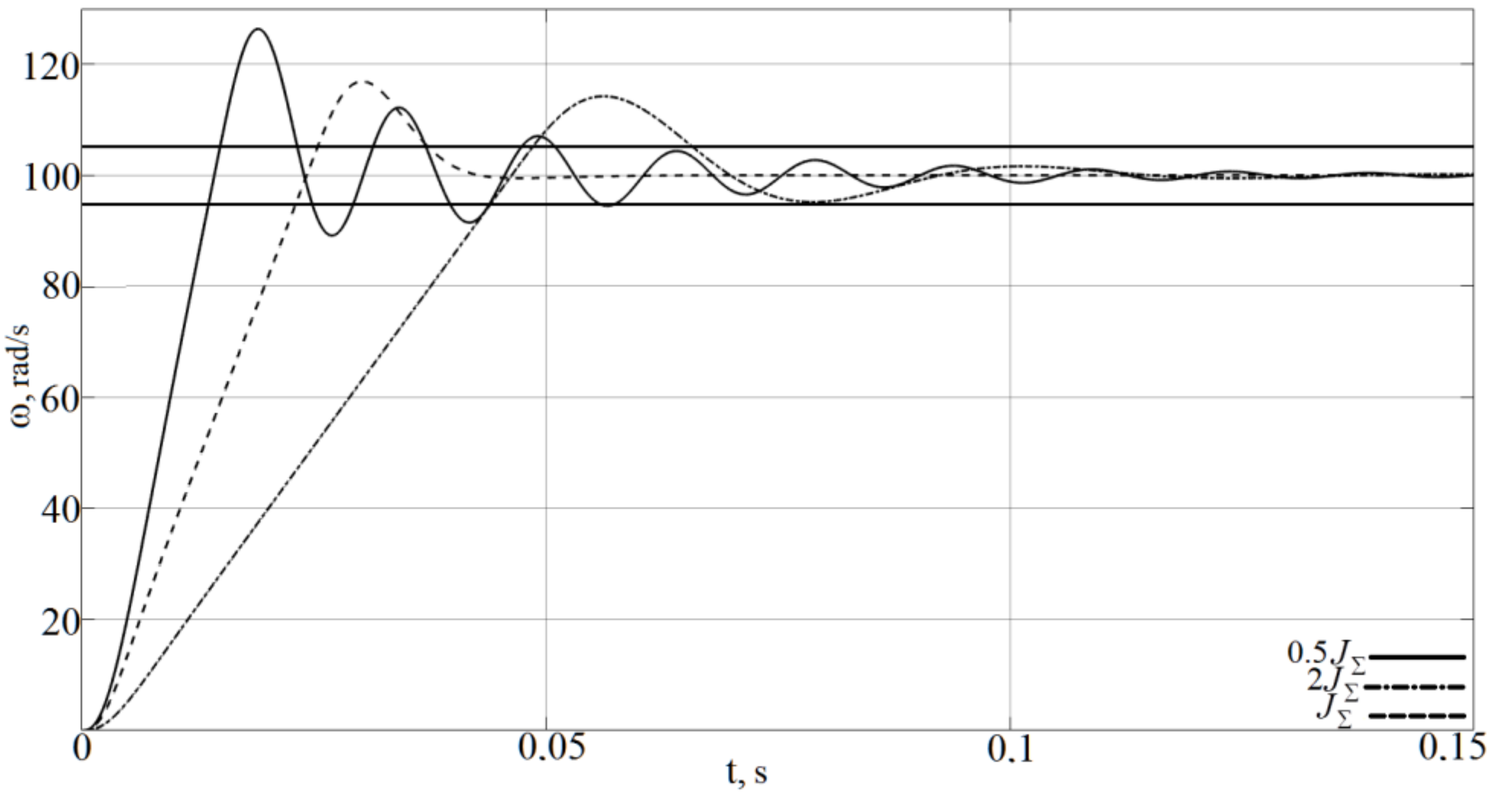
Figure 4 shows a comparison of the speed transient curves obtained from the cascade control system of the DC drive. The experiments were conducted with the mathematical model of the electric motor described above. Three curves are shown. The first (ideal) one was obtained under the condition that all the parameters had their nominal values, the second one—under the condition that the value of the inertia moment was doubled, whereas the third one—when it was halved in comparison with the nominal value. At the same time, the armature resistance and inductance were also increased by a factor of 1.5 compared to their nominal values.

Considering the experiment with the doubled inertia moment, the speed settling time increased by 22.1 milliseconds and overshoot decreased by 2.58%, as compared to the ideal ($J_{\Sigma }$) output curve. This can be explained by taking into account the motor armature current limits [−1 A; 1 A]. Because of them, the motor accelerated with bounded maximum acceleration. In the idle mode (no load torque), its value can be found from the electric drive model by Equation (26).

$$\frac{d\mathsf{\omega }}{dt}=\frac{c{\Phi }_e}{2J_{\Sigma }}{u}_{max}$$

(26)

Thus, if the inertia moment is increased compared to the nominal value, or any other situation when the motor accelerates with constant acceleration occurs, then the transient with maximum possible rate, but without the overshoot and oscillations, is considered to be the best one.

The experiment, which is shown in Figure 4, also indicated that when the inertia moment was lower than its nominal value, the speed settling time was decreased by 9.95 milliseconds, the overshoot was increased by 9.5%, and three damped oscillations occurred. In this case, a transient, which coincided with the ideal one ($J_{\Sigma }$), was considered to be the best possible one. The values of the control quality indices (the overshoot $\sigma$, the settling time $t_{settle}$, and the number of oscillations n) of the transients (Figure 4) are shown in

Table 1. Control quality indexes.

Plant	$\mathit{\sigma }$, %	${\mathit{t}}_{\mathit{s}\mathit{e}\mathit{t}\mathit{t}\mathit{l}\mathit{e}}, \mathbf{s}$	n
Nominal values	16.8	0.0243	0
0.5 $J_{\Sigma }$/1.5 R/1.5 L	26.3	0.01435	3
2 $J_{\Sigma }$/1.5 R/1.5 L	14.2	0.0464	1

.

It follows from Table 1 and Figure 4 that the conventional cascade control system was not able to keep the ideal ($J_{\Sigma }$ curve) control quality due to the above-described non-stationarities. Thus, the adaptive system application is relevant.

The further experiments were of three types. The first one was to model the influence of the load torque ${\mathsf{\tau }}_e\ne 0$ when there was no parameter uncertainty ${\widehat{K}}_{ref}\left(0\right)-K_{ref}=0$. The second one was to model the vice versa situation: ${\mathsf{\tau }}_e=0$, ${\widehat{K}}_{ref}\left(0\right)-K_{ref}\ne 0$ and $\widehat{K}\left(0\right)-K\ne 0$. The third one was to model the influence of both the load torque ${\mathsf{\tau }}_e\ne 0$ and the parameter uncertainty ${\widehat{K}}_{ref}\left(0\right)-K_{ref}\ne 0$ and $\widehat{K}\left(0\right)-K\ne 0$.

The parameters of the reference model were calculated according to the Equation (11), the matrix $Q$ in (18) was chosen as unity one, and the initial values of the speed controller and the reference model correction parameters were calculated according to the nominal values of the motor parameters:

$${\widehat{K}}_I\left(0\right)=\frac{J_{\Sigma }}{c{\Phi }_e{a}_{\mathsf{\omega }}{a}_I^3{T}_{\mathsf{\mu }}^2}; {\widehat{K}}_P\left(0\right)=\frac{J_{\Sigma }}{c{\Phi }_e{a}_I^2{T}_{\mathsf{\mu }}^{-1}}; {\widehat{K}}_{ref}\left(0\right)=\frac{c{\Phi }_e}{10J_{\Sigma }}$$

(27)

The transfer functions $H_1\left(p\right),\hspace{0.33em}{H}_2\left(p\right)$ for the plant under consideration took the form:

$$H_1\left(p\right)=\frac{3.5979p+0.0288}{3.2\times {10}^{-5}{p}^2+0.008p+1}; H_2\left(p\right)=\frac{0.002p+1.6\times {10}^{-5}}{p^2+250p+31250}.$$

(28)

The poles and zeros of these transfer functions are negative, and their relative degree is one, so they are strictly positive real.

3.2. First Experiment

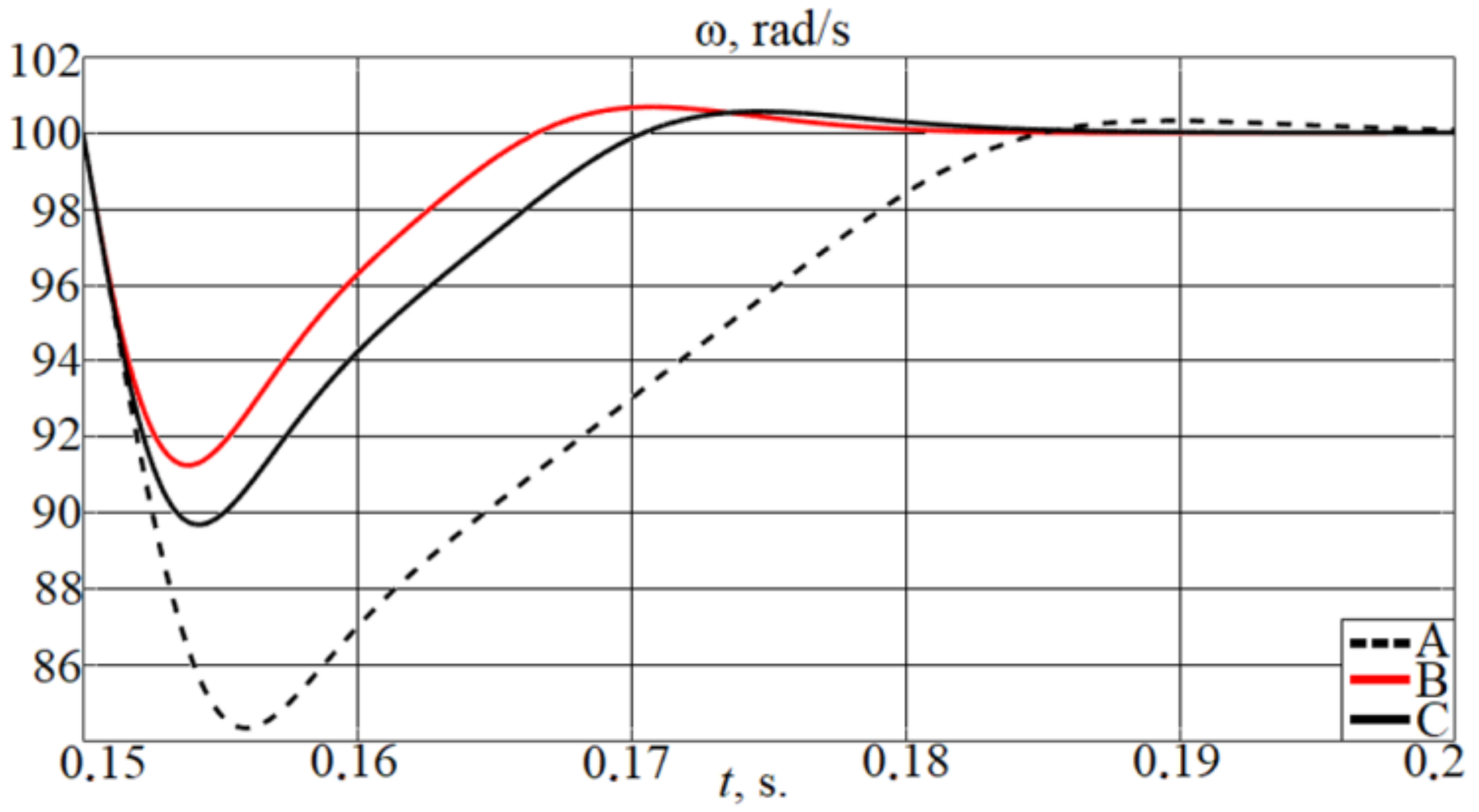
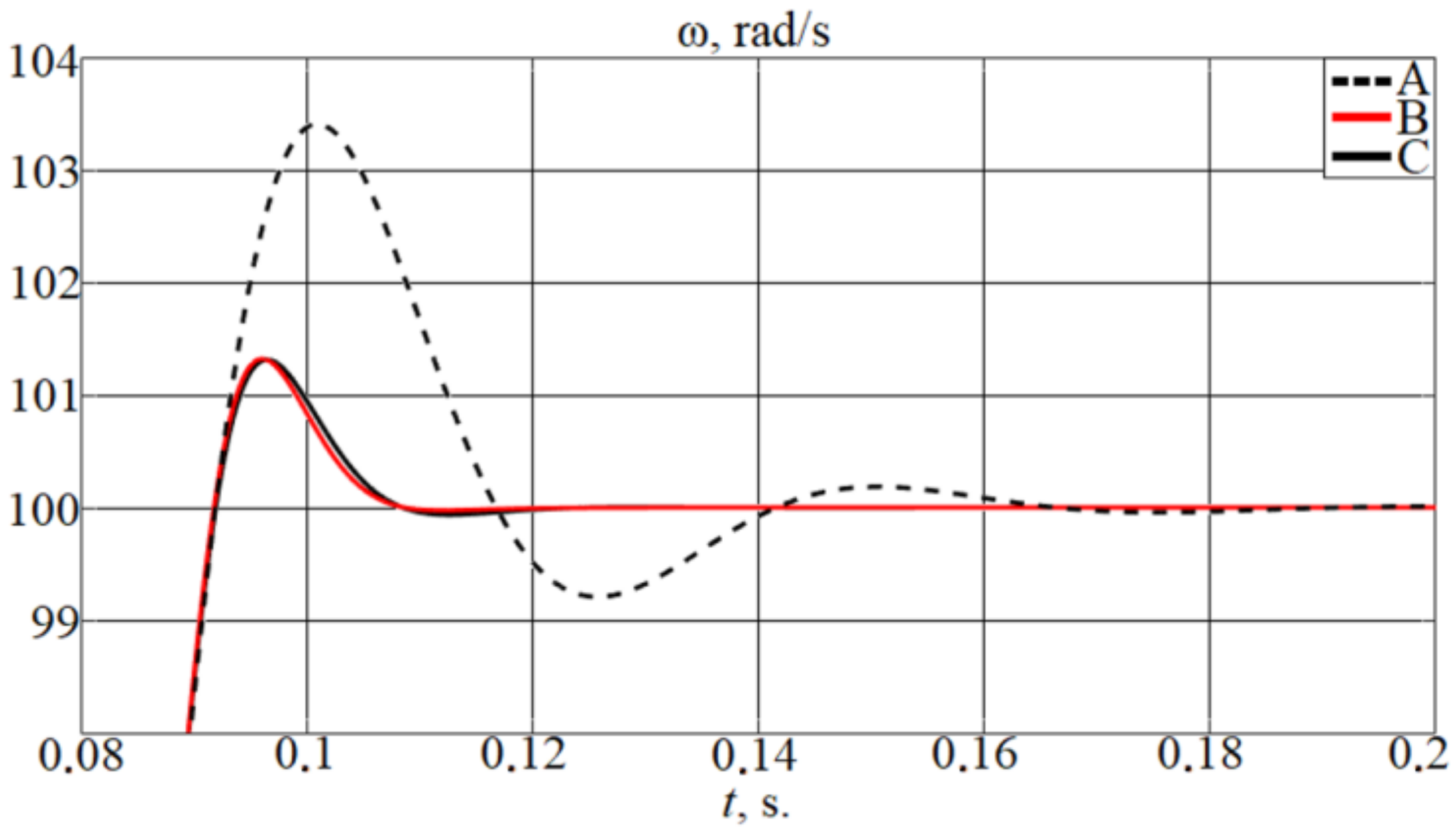
A constant signal $r_{\mathsf{\omega }}$ = 100 rad/s was used as the speed setpoint. All the motor parameters had their nominal values, thus the adaptive laws for ${\widehat{K}}_{ref}$ and $\widehat{K}$ were not used (${\dot{\tilde{K}}}_{ref}=0$ and $\dot{\tilde{K}}=0$). The gains of the adaptive law for ${\widehat{u}}_{ad}$ were chosen as ${\gamma }_1^I=12\times {10}^4$, ${\gamma }_1^P={10}^2$. The load torque was modeled with the help of the following function:

$$M_c=0.07h\left(t-0.15\right),$$

(29)

where $h\left(t-0.15\right)$ is the unit-step function at the time point $t$ = 0.15 s.

Figure 5 shows the speed $\mathsf{\omega }$ curves obtained from: (1) the conventional cascade control system without adaptation—(A), (2) the system with a priori knowledge (ideal case) of the load torque function (29)—(B), and (3) the developed adaptive system—(C). The speed controller parameters for the conventional cascade control system were calculated in accordance with (3).

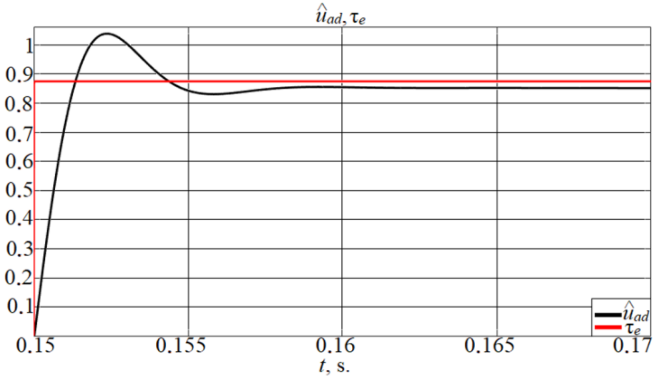
The ideal value of ${\mathsf{\tau }}_e$ and the obtained transient of its estimation ${\widehat{u}}_{ad}$ are shown in Figure 6.

As follows from Figure 5 and Figure 6, the developed system approximated the value of disturbance ${\mathsf{\tau }}_e$ with sufficient accuracy and fast response. These resulted in the improvement of the quality of ${\mathsf{\tau }}_e$ compensation by the control system.

3.3. Second Experiment

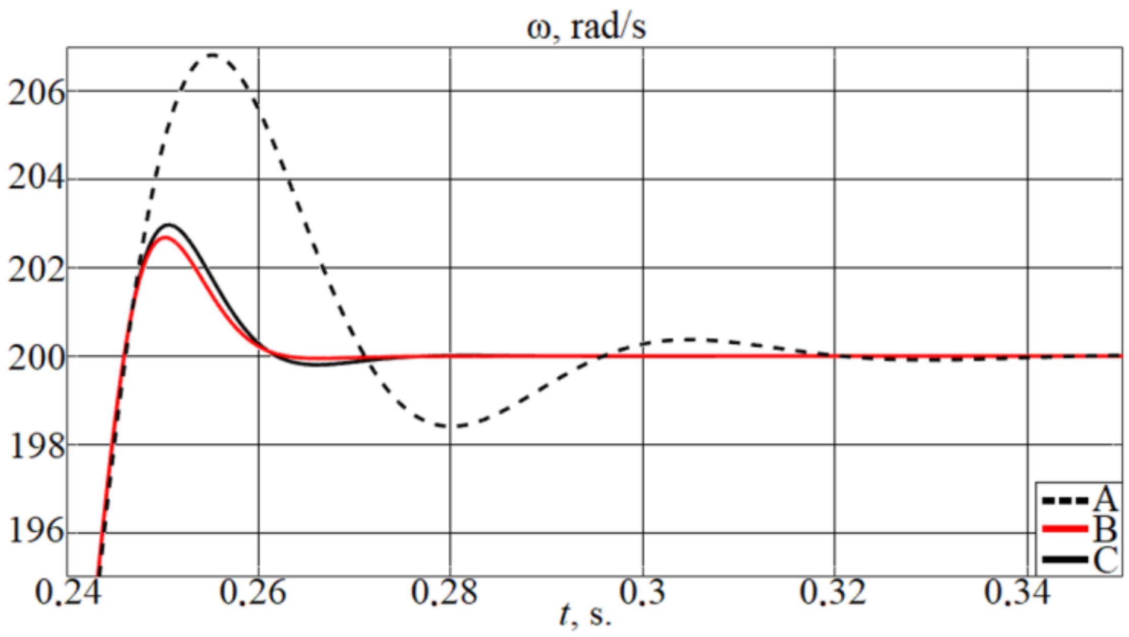
The motor speed setpoint $r_{\mathsf{\omega }}$ was a piecewise-continuous function, which was implemented as a cycle of the drive acceleration to 200 rad/s and after 0.2 s its deceleration to 100 rad/s, and so on. The duration of the experiment was 2 s. It contained 10 transients according to the above-described setpoint schedule. The load torque was equaled to zero, so the adaptive law for ${\widehat{u}}_{ad}$ was not used (${\dot{\tilde{u}}}_{ad}=0$). The motor inertia moment $J_{\Sigma }$ was doubled. The parameters ${\gamma }_2^I,{\gamma }_2^P$ and the gain matrices ${\Gamma }_P,{\Gamma }_I$ were chosen, as follows:

$${\Gamma }_I=\left[\begin{array}{cc}5\times {10}^4& 0\\ 0& 1,2\end{array}\right]; {\Gamma }_P=\left[\begin{array}{cc}50& 0\\ 0& 1,2\times {10}^{-3}\end{array}\right]; \begin{array}{c}{\gamma }_2^I=4\times {10}^5;\\ {\gamma }_2^P=4\times {10}^2.\end{array}$$

(30)

Figure 7 shows a comparison of the second transient of the motor speed $\mathsf{\omega }$ to 200 rad/s obtained from: the conventional cascade control system without adaptation—(A), the system with the speed controller parameters calculated for the doubled value of the inertia moment (ideal curve) with the help of (27)—(B), and the developed adaptive system—(C).

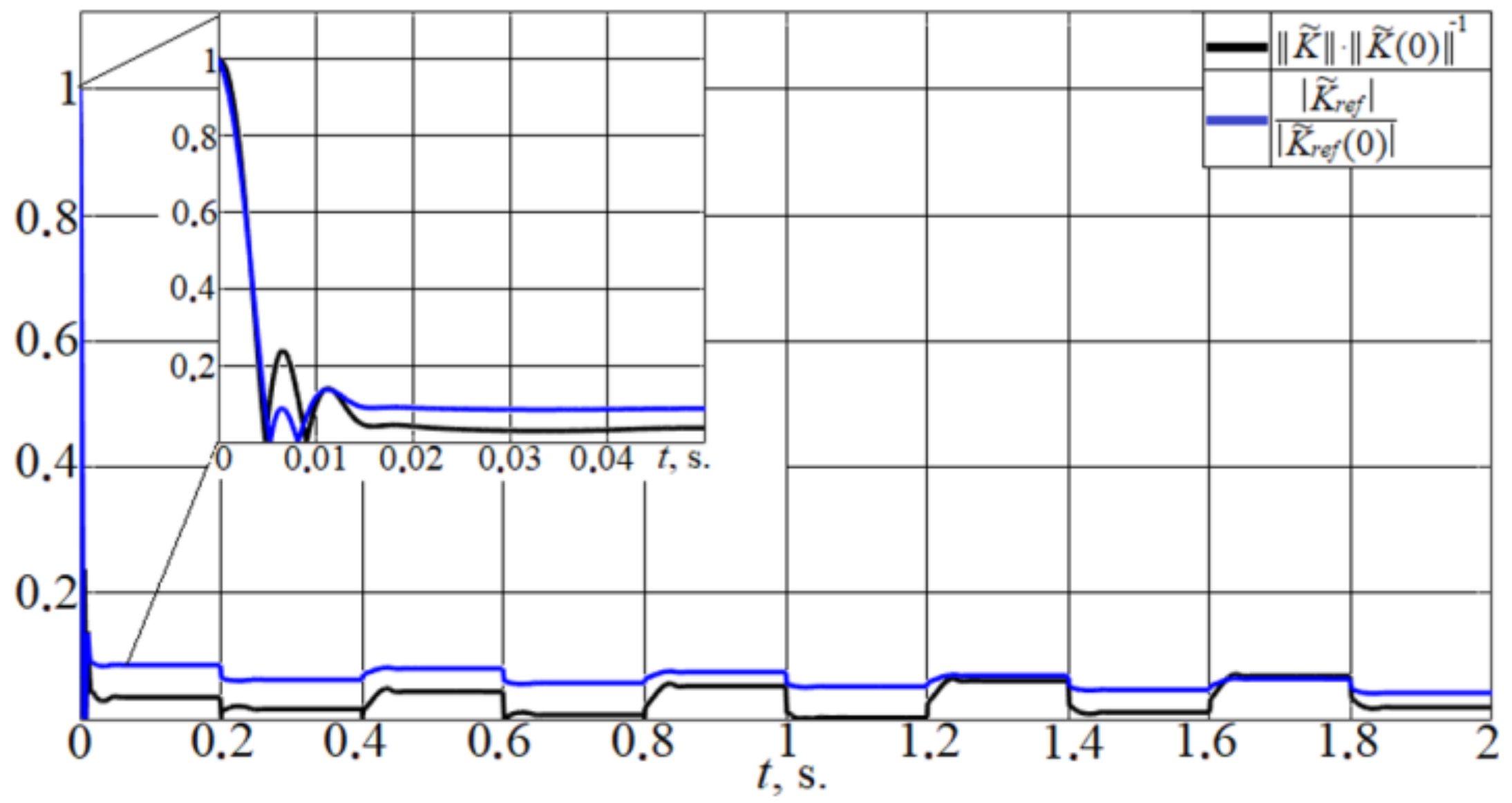
Figure 8 shows the transient curves of $\left|{\tilde{K}}_{ref}\right|\left|{\tilde{K}}_{ref}^{-1}\left(0\right)\right|$ and $‖\tilde{K}‖\cdot {‖\tilde{K}\left(0\right)‖}^{-1}$. The ideal values of these parameters were calculated using (27).

As follows from Figure 7 and Figure 8, the developed system estimated the ideal parameters of the speed controller with sufficient accuracy, which made it possible to significantly improve the quality of the motor speed control after just one cycle 100–200–100 rad/s of the setpoint schedule.

3.4. Third Experiment

The setpoint schedule was the same as in the course of the second experiment.

The load torque value was chosen as $M_c=0.04$. The inertia moment $J_{\Sigma }$ value was doubled in comparison with the nominal one. The parameters ${\gamma }_2^I,{\gamma }_2^P$ and matrices ${\Gamma }_P,{\Gamma }_I$ were chosen according to (30), whereas the adaptive gains of the adaptive law ${\widehat{u}}_{ad}$ were ${\gamma }_1^I=12\times {10}^2$, ${\gamma }_1^P=1$.

Figure 9 demonstrates the comparison of the first transient of $\mathsf{\omega }$ obtained from the cascade control system: (1) without adaptation—(A), (2) in which the speed controller parameters were initially calculated under the condition that we knew that the inertia moment was doubled and $M_c=0.04$—(B), (3) with the proposed adaptive laws—(C).

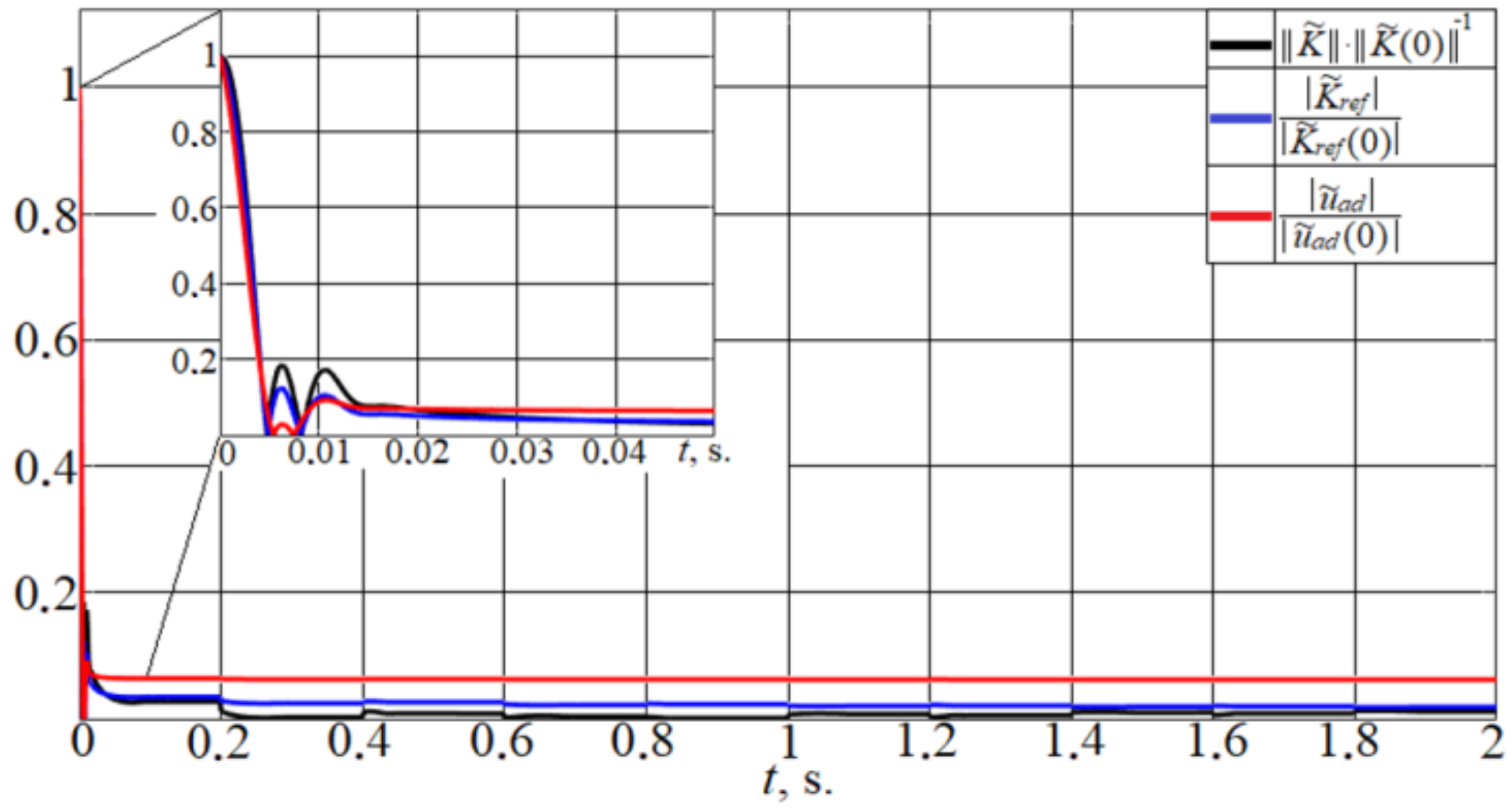
The transient curves of $\left|{\tilde{K}}_{ref}\right|\left|{\tilde{K}}_{ref}^{-1}\left(0\right)\right|$, $\left|{\tilde{u}}_{ad}\right|\left|{\tilde{u}}_{ad}^{-1}\left(0\right)\right|$ and $‖\tilde{K}‖\cdot {‖\tilde{K}\left(0\right)‖}^{-1}$ are shown in Figure 10 (the ideal values were calculated using (27)).

As follows from Figure 9 and Figure 10, the developed system estimated the ideal parameters of the speed controller and load torque with sufficient accuracy to improve the quality of the motor speed control.

4. Conclusions

The adaptive control system of the DC motor speed, which consisted of a PI-controller with dynamically adjustable parameters and an adaptive compensator for the motor load torque, was developed in this research. In this system, the proposed reference model correction method took into account both the boundedness of the control signal and the unmodeled dynamics of the armature current loop. The obtained adaptive laws allowed it to meet Popov’s hyperstability criterion for the closed-loop adaptive control system. The experiments demonstrated that the developed system effectively compensated for the influence of the load torque and the inertia moment variations on the control quality of the DC motor speed. The obtained system can be recommended for practical implementation within a unified industrial thyristor DC drives.

References

- Leonard, W. Control of Electrical Drives, 3rd ed.; Springer Science & Business Media: Berlin, Germany, 2001; ISBN 978-3-642-97646-9. [Google Scholar]
- Saidur, R. A review on electrical motors energy use and energy savings. Renew. Sustain. Energy Rev. 2010, 14, 877–898. [Google Scholar] [CrossRef]
- Bortsov, Y.A.; Polyakhov, N.D.; Putov, V.V. Electromechanical Systems with Adaptive and Modal Control; Energoatomizdat: Leningrad, Russia, 1984. (In Russian) [Google Scholar]
- Umland, J.W.; Safiuddin, M. Magnitude and symmetric optimum criterion for the design of linear control systems: What is it and how does it compare with the others? IEEE Trans. Ind. Appl. 1990, 26, 489–497. [Google Scholar] [CrossRef]
- Eremenko, Y.; Glushchenko, A.; Petrov, V. On PI-controller parameters adjustment for rolling mill drive current loop using neural tuner. Procedia Comput. Sci. 2017, 103, 355–362. [Google Scholar] [CrossRef]
- Fan, L.; Liu, Y. Fuzzy self-tuning PID control of the main drive system for four-high hot rolling mill. J. Adv. Manuf. Syst. 2015, 14, 11–22. [Google Scholar] [CrossRef]
- Glushchenko, A.I.; Petrov, V.A.; Lastochkin, K.A. Method Development of Speed Control of DC Drive on Basis of Its Feedback Linearization. In Proceedings of the European Control Conference, Saint-Petersburg, Russia, 12–15 May 2020. [Google Scholar] [CrossRef]
- Glushchenko, A.I.; Petrov, V.A.; Lastochkin, K.A. Reference Model Hedging under Conditions of Bounded Control Action Signal to Implement Adaptive Control of DC Drive. In Proceedings of the International Conference on Control Systems, Mathematical Modeling, Automation and Energy Efficiency, Lipetsk, Russia, 11–13 November 2020. [Google Scholar] [CrossRef]
- Landau, I.D. A hyperstability criterion for model reference adaptive control systems. IEEE Trans. Autom. Control. 1969, 14, 552–555. [Google Scholar] [CrossRef]
- Fradkov, A. Passification of non-square linear systems and feedback Yakubovich-Kalman-Popov lemma. Eur. J. Control. 2003, 9, 577–586. [Google Scholar] [CrossRef]
- De La Sen, M. Stability of composite systems with an asymptotically hyperstable subsystem. Int. J. Control. 1969, 44, 1769–1775. [Google Scholar] [CrossRef]
- Marquez, H.J.; Damaren, C.J. On the design of strictly positive real transfer functions. IEEE Trans. Circuits Syst. I Fundam. Theory Appl. 1995, 42, 214–218. [Google Scholar] [CrossRef] [Green Version]
- Karason, S.P.; Annaswamy, A.M. Adaptive control in the presence of input constraints. In Proceedings of the American Control Conference, San Francisco, CA, USA, 2–4 June 1993. [Google Scholar] [CrossRef] [Green Version]
- Popov, V.M. The solution of a new stability problem for controlled system. Autom. Remote Control. 1963, 24, 1–23. [Google Scholar]
- Ioannou, P.A.; Sun, J. Robust Adaptive Control; Courier Corporation: Chelmsford, MA, USA, 2012; ISBN 978-0486498171. [Google Scholar]
Figure 1.
DC drive cascade control system scheme.
Figure 2.
Plant of DC drive speed control loop.
Figure 3.
Transformed scheme of plant of DC drive speed control loop.
Figure 4.
Speed transient curves obtained from conventional cascade control system.
Figure 5.
Comparison of motor speed curves when and .
Figure 6.
Comparison of with .
Figure 7.
Comparison of motor speed curves when , and .
Figure 8.
Comparison of transient curves of normalized errors and .
Figure 9.
Comparison of transients of motor speed when , and .
Figure 10.
Comparison of transients of normalized errors.