
Green Ammonia Production in Stochastic Power Markets


1
School of Computing and Mathematical Sciences, Birkbeck, University of London, London WC1E 7HX, UK
2
Centrica Energy, Skelagervej 1, 9000 Aalborg, Denmark
3
Department of Applied Mathematics and Statistics, Johns Hopkins University, Baltimore, MD 21218, USA
4
Ralph O’Connor Sustainable Energy Institute (ROSEI), Johns Hopkins University, Baltimore, MD 21211, USA
5
Business School, University of Inland, Vormstuguvegen 2, 2624 Lillehammer, Norway
*
Author to whom correspondence should be addressed.
Commodities 2024, 3(1), 98-114; https://doi.org/10.3390/commodities3010007
Submission received: 9 February 2024
/
Revised: 28 February 2024
/
Accepted: 29 February 2024
/
Published: 6 March 2024
Abstract
:Real assets in the energy market are subject to ecological uncertainty due to the penetration of renewables. We illustrate this point by analyzing electrolyzers, a class of assets that recently became the subject of large interest, as they lead to the production of the desirable green hydrogen and green ammonia. The latter has the advantage of being easily stored and has huge potential in decarbonizing both the fertilizer and shipping industries. We consider the optimization of green ammonia production with different types of electricity procurement in the context of stochastic power and ammonia markets, a necessary assumption to translate the features of renewable, hence intermittent, electricity. We emphasize the importance of using stochastic prices to model the volatile nature of the price dynamics effectively, illustrating the project risks that hedging activities can mitigate. This study shows the pivotal role of flexibility when dealing with fluctuating renewable production and volatile electricity prices to maximize profits and better manage risks.
1. Introduction
The European electricity market is confronted with the critical task of meeting escalating energy demand while simultaneously decreasing its carbon footprint. The existing electricity mix predominantly relies on fossil fuels, which are the principal contributors to greenhouse gas emissions [1]. The need for more energy and the urgency to decarbonize the power sector has driven the adoption of renewable energy sources, such as wind, solar, and hydropower, where possible. However, the inherent volatility of electricity augmented by the intermittent nature of solar and wind has led to grid instability and price cannibalization [2], emphasizing the need for a more flexible and intelligent grid capable of balancing supply and demand in real time, with storage facilities not achieved yet in terms of size and duration by existing battery solutions.
Power-to-X (PtX) technology has recently emerged as a promising solution to these challenges. PtX encompasses the conversion of surplus renewable electricity into various energy carriers, including hydrogen, methane, and synthetic fuels. The European Commission estimates that to reach net-zero emissions by 2050, as much as 200 Mtonnes of hydrogen production per year should already be achieved by 2030 [3]. The production of green fuels through PtX would enable the European Union to reduce its dependence on fossil fuels, enhance energy storability, and ensure electricity supply when demand surpasses renewable energy generation. As an example, the German utility RWE—which cannot rely anymore on Russian natural gas—is building two electrolyzer plants in Norway that will be powered by offshore wind from the North Sea and produce hydrogen, which will be then transported to Germany by hydrogen pipeline between Norway and Germany [4]. The two projects are part of RWE’s efforts to build a total of 300 MW of electrolyzer capacity in Lingen by 2026 [5].
Hydrogen, generated through electrolysis using renewable energy sources, is considered a clean and efficient fuel for transportation. It is viewed as a necessary step to reach net-zero CO2 emissions [6,7]. According to the International Energy Agency (IEA), the use of hydrogen and ammonia will reach almost 3.5 GW of potential capacity by 2030, counting all the projects under development around the globe [8]. Additionally, the development of advanced and cost-effective storage technologies is crucial for hydrogen’s broad development in the transportation sector.
Ammonia, produced through nitrogen fixation and hydrogenation, has major applications in the agricultural and transport industries. As a fuel, ammonia boasts a higher energy density than hydrogen and is compatible with internal combustion engines. Ammonia is also one of the three traditional fertilizers, and as of today, its production accounts for 2% of the global CO2 emission [9]. Converting the current ammonia production to a greener one holds significant potential for reducing greenhouse gas emissions in agriculture [10]. Outside fertilizers, ammonia can act as a hydrogen carrier, addressing storage and distribution challenges. A 2021 World Bank report observes that ammonia is preferable to hydrogen to replace bunker fuels, in particular for long-distance transport and storage [11,12]. Many projects ranging from boilers [13] to cotton farming [14] have been announced where green ammonia would be used as a major tool towards carbon neutrality.
The feasibility of those projects is highly dependent on their rentability. In [15], the overseas hydrogen supply chain for different countries was investigated, where future electricity prices were modeled by exponential decay regression with bounded values based on historical data. This method has the shortcomings of relying heavily on historical data (i.e., the forecast strongly depends on the choice of the historical window) and leaning on a single price time series, which can be heavily biased. Techno-economic assessment of green ammonia production was performed in [16,17]. Salmon et al. [16] investigated offshore green ammonia production where the generating assets were co-located with the production plant and isolated from the grid, removing the possibility of optimizing revenue generated from selling electricity and thus reducing flexibility. Campion et al. [17] used a similar model with different wind and solar potentials in different locations in the world but added the possibility of supplying extra electricity with a connection to the grid. In this case, electricity prices from the single year 2019 were used, where the price level was significantly lower than the current one. Relying on a single year or a single outcome is an unrealistic assumption at this moment, given the uncertainty created by the climate transition and the consequences of wars on the world economy. In fact, the literature recognizes the necessary stochastic nature of electricity prices—with increased uncertainty brought by intermittent renewables, including the quasi-stochastic market clearing [18]. Furthermore, the profit distributions generated by stochastic scenarios offer a meaningful tool to support the design of hedging activities, which can ultimately reduce a project’s risks.
Instead, this study presents the optimization of the production of green ammonia under stochastic electricity and ammonia prices for different plant configurations and with electricity provided via different structures. Fixed costs and operational expenses are omitted with the purpose of isolating the system’s sensitivity to parameters directly impacting the plant’s performance.
The optimization model of the Power-to-X production is first described, followed by our proposed stochastic modeling of electricity and ammonia prices. The results of the optimization model are then discussed, in particular, some relevant statistics on expected revenues and risks for green ammonia production projects.
2. Methodology
2.1. Power-to-NH3 Production Model
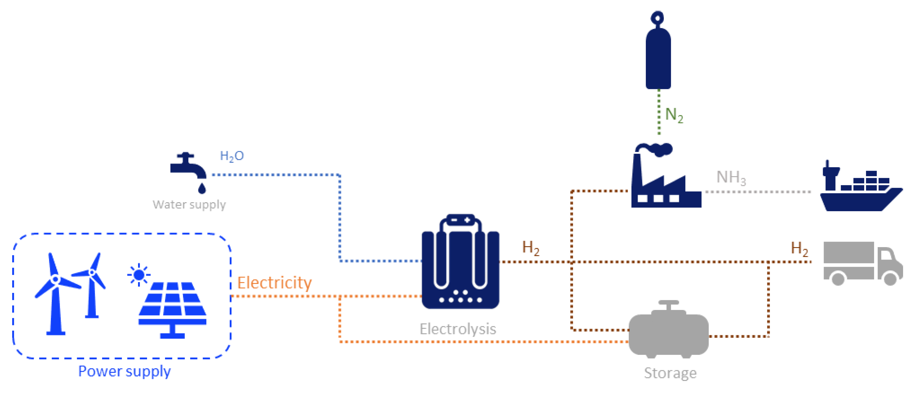
Since the first half of the 20th century, the main industrial process used for producing ammonia has been the Haber–Bosch process [19]. In this process, nitrogen (N2), which is commonly present in the air, is combined with hydrogen (H2) under high pressure and high temperatures to produce ammonia (NH3). N2 is easily filtered from the atmosphere, but H2 is more difficult to obtain. Methane from natural gas is the most commonly used hydrogen source. A steam reforming process is used to separate the carbon and hydrogen atoms, where CO2 is released as a by-product or waste. To produce ammonia without CO2 waste or, in other words, green ammonia, hydrogen should be produced sustainably. Splitting water molecules by electrolysis using power from renewable energy sources is one of the most promising avenues to produce green hydrogen. The process of producing green fuel (hydrogen, ammonia, etc.) using power from renewable energy sources has been recently termed a Power-to-X process, where X refers to the output, i.e., hydrogen, ammonia, or other.
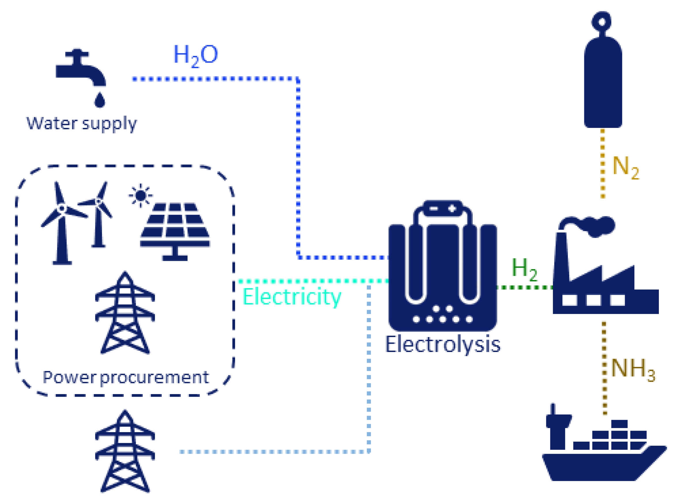
A Power-to-X plant producing green hydrogen and green ammonia is represented in Figure 1. Different options are available to feed such a plant with certified green electricity. The plant can be directly co-located with green generating assets, like a wind farm and/or a solar farm. Another option is to enter a power purchase agreement (PPA), with corresponding green certificates ensuring that power is coming from renewable sources, delivered either as an as-produced profile from the renewable assets or a constant profile (also referred to as baseload profile). In general, these options can also be combined. For example, a PPA can be purchased for a co-located configuration (also referred to as an island configuration) in order to supplement the plant with additional electricity and increase the production of hydrogen or ammonia.
Several challenges are linked to running a Power-to-X plant: (i) in the case of as-produced profiles for the power supplied, the electricity input fluctuates and its quantity is difficult to forecast; (ii) some of the processes involved are more or less flexible in terms of load ranges, ramp-up and -down capabilities and power consumption; and (iii) in some configurations, it may be quite profitable to sell excess power to the local grid when spot prices are high, adding some complexity to the model at times of high volatility of electricity prices.
In this study, we consider the problem of a Power-to-X plant that produces green ammonia and identify the parameters that impact profitability the most. To maximize the production output of a Power-to-NH3 plant while ensuring its profitability, the problem is defined as an optimization problem. The objective of the optimization is to maximize the profit and loss (P&L) of the plant, which is defined as:
where is the amount of power sold to the grid in MW, is the power bought from the grid in MW, is the spot price of the power in EUR/MWh, is the quantity of power procured in MW, is the price of electricity provided through the PPA in EUR/MWh, is the normalized electrical loss associated with the electrical installation of the plant, is the quantity of produced in tonnes, is the selling price of in EUR/tonnes of and t is the unit of time of the problem. Constraints are obviously present, and the problem can then be formulated as:
subject to the following constraints:
where
- N is the total number of hours in the optimization period
- is the power sold back to the grid at time t in MWh
- is the power provided through a PPA contract or off-grid connection to a generating asset at time t in MWh
- is the power bought from the grid at time t in MWh
- is the normalized electrical loss associated with the plant
- is the spot price when selling/buying power at time t in EUR/MWh
- is the price of electricity provided through the PPA in EUR/MWh
- is the quantity of NH3 produced at time t in tonnes of NH3
- T is the total time for the NH3 contract
- is the quantity of H2 produced at time t in tonnes of H2
- is selling price of NH3 at time t in EUR/tonnes of NH3
- is the minimal production capacity of the NH3 process (set to 0.2, i.e., the process cannot run at a lower load than 20% of the maximum load)
- is the maximal hourly capacity of the NH3 process in tonnes of NH3
- is the NH3 contract in tonnes of NH3
- is the total power used to produce NH3 at time t in MWh
- is the power used by the electrolyzer at time t in MWh
- is the power used for the water treatment at time t in MWh
- is the power used by the NH3 process at time t in MWh
- is the energy consumption for the electrolyzer to convert electricity into H2 in MWh/t of H2
- is the energy requirement for the water treatment in MWh/tonnes of H2
- is a binary variable for the production of NH3 at time t i.e., its value is 1 when NH3 is produced and 0 when not
- is the power consumed by the NH3 process when producing NH3 in MWh
- is the power consumed by the NH3 process when in standby in MWh
- is the mass balance between NH3 and H2
- is the mass balance between H2O and H2
- is the grid connection limit in MW.
The parameters and variable optimized are listed in Table A1.
The formulation of the problem is expressed using the Pyomo Python package [20] and solved with the SCIPY solver [21]. Some assumptions were made in order to keep the computational time reasonable for the number of scenarios:
- The power consumption of the electrolyzer is approximated to be linear with respect to the load. In reality, the load curve of an electrolyzer is not linear, as optimal working conditions are typically at 80% of full load. The results will be slightly more optimistic than reality, but the effect should be minimal and relatively constant throughout the different scenarios.
- The power consumption of the Haber–Bosch is modeled using two levels: when the unit is producing and when the unit is on standby. This simplistic modeling approach is more restrictive than realistic working conditions, as higher efficiency rates should be attainable as load increases.
- The plant cannot buy and sell power at the same t. This reflects what would happen in reality.
- Only the renewable power can be sold to the grid. As the plant cannot buy and sell at the same t, this means only the power produced by the renewable assets or the power provided through the PPA can be sold to the grid.
The input parameters used in the model are listed in Table 1. The electricity prices for Germany presented in Section 2.2 are used as inputs for the spot prices (). The year 2020 was used for solar production as it yielded close to median production. The production from 2020 was repeated for three years, the total period of the optimization. In principle, each price scenario should be linked to a specific renewable production pattern, but uncertainties in weather forecasts over the years are high. Therefore, an average year over many scenarios was used instead. The problem could have been extended to a four parameters stochastic process (price, volatility of price, wind production, and solar production), adding, however, complexity not necessary given the scope of this study, which is to compare the power procurement scenarios and identify the parameters to which optimal outputs are more sensitive. The expected price for NH3 () is described in Section 2.3.
2.2. Electricity Prices Model
To model electricity prices used as input for the production model, we propose a one-factor model [22,23]. To ensure positivity while avoiding the geometric Brownian motion (which increases in average and is therefore inappropriate for electricity prices), we assume that the -spot price follows an Ornstein-Ulenbeck (OU) process [22,24]. Besides its mean-reverting property, the OU process leads to a normal distribution for all -spot prices and a closed-form solution for -forward prices, hence a precise calibration of the model. Following [25] we place ourselves directly under the pricing measure and write the dynamics of as
where is the long-term mean -spot price, k is the speed of adjustment, is the volatility of the process and is a Brownian motion under the measure . Equation (4) integrates as
where is the initial -spot price.
Moreover, we know that the conditional distribution of X at time t under the measure is normal with
where , and S the spot price at time t log-normally distributed under .
Let us now move to the forward price of the commodity with maturity T. Assuming constant interest rates, the forward price with maturity T is the expectation of the spot price at time T under the measure
and from the properties of the log-normal distribution, we have
Finally, substituting from Equation (5) and using Equation (6) we obtain, in log form
which is used for the calibration of the model.
2.2.1. Electricity Price Model Calibration
In the case of commodities, one of the difficulties in the empirical calibration is that the state variable, i.e., the spot price, is not directly observable. On the other hand, Futures contracts are widely traded, and their high liquidity makes their prices easily observable. The state space model, as discussed in [26], is, in fact, the appropriate tool to deal with state variables that are unobservable but generated by a Markov process. The Kalman filter can be applied to the model in its state space form to estimate the unobserved parameters and k.
Following [22,26], the measurement equation is obtained by adding to Equation (6) serially and cross-sectionally uncorrelated disturbances with mean zero so that we take into account bid-ask spreads, price limits, and errors in the data. The measurement equation relates the time series of observable variables, in our case, forward prices for different maturities, to the unobservable state variable, the spot price. Based on this, from Equation (6), we write the measurement equation as
where
- , , vector of observables,
- vector,
- vector,
- vector of serially uncorrelated disturbances with and .
The next step is to generate the unobserved state variable via the transition equation, which is a discrete-time version of the stochastic process in Equation (4). We can, therefore, write the transition equation as
where
- , serially uncorrelated disturbances with and .
The Kalman filter is then applied as a recursive procedure to compute the optimal estimator of the state variable at time t, based on the information at time t, and updated continuously as new information becomes available. To apply the simple Kalman filter, we assume that both the disturbances and the initial state variable are normally distributed; we can, therefore, calculate the maximum likelihood function and estimate the model parameters and k.
2.2.2. Model Implementation
We calibrate the model using Future contract closing prices. As said before, the reasons for using Future prices instead of spot (or day-ahead) are tied to the characteristics of the electricity markets, namely non-storability and the hourly settlement (set to be reduced to 15 min in most EU markets in the future). In particular: (i) the spot price can be extremely volatile in its hourly granularity, as it is very sensitive to imbalances between supply and demand; (ii) in markets with high renewables penetration, volatility is especially high as in the short term the generation from renewables (wind in particular) can vary substantially from the expected volumes; (iii) the Futures market is in general a better and more stable representation of the medium-term (i.e., beyond monthly) market development; (iv) the maturities that we will use for the calibration (front month to year 3) are very liquid contracts in the reference market (i.e., Germany), with daily settlement historical data easily available.
Using the German market and closing prices from the European Power Exchange (EEX) [27], we calibrate the model using the Kalman Filter (see Section 2.2.1) and proceed as follows:
- We collect daily settlement prices of M1, Q1, Y1, Y2, Y3 Future contracts, where M1 refers to front month, Q1 front quarter, Y1 front year, Y2 front year +1, Y3 front year +2.
- The data period was 1 July 2002 to 18 April 2023. The entire available series was used to remove bias from choosing a specific calibration window, especially given the very volatile period of 2021 and 2022. As we are interested in the volatility and mean reversion speed of (log) returns, we considered using a long historical period as the most robust option, also to reduce sensitivity to localized market shocks, while still attributing more weight to recent observation thanks to the feature of the Kalman filter.
- We calibrate the state space model presented in Section 2.2.1 to estimate the parameters k and , used in Equation (9) to generate future electricity prices.
Finally, we run the model using the following parameters:
As a result, a 750 (days) × 4000 (scenarios) matrix of prices is generated. Since we are modeling renewables, we are interested in the shape of intraday prices. To increase the granularity of our data from daily to hourly and introduce daily shapes, we use historical hourly ratios calibrated on the last two years of historical hourly prices - the two years depicting the recent generation mix development, in particular the recently higher renewable penetration. We finally multiply the 24 (hours) × 365 (days) historical hourly ratios with each 750 days-scenario, thus obtaining 4000 scenarios of 18,000 h.
2.3. Ammonia Price Model
As with what we have observed with electricity generated by renewables, we expect that green ammonia will trade at a premium in the short to mid-term compared to gray ammonia (i.e., ammonia generated from gas), with the main driver of such a premium being:
- A growing demand for green ammonia as a critical tool that will be adopted, for example, to decarbonize transport and agricultural industries.
- The premium currently charged to certify renewable energy (e.g., Guarantees of Origin in Europe) will be transferred to the price of ammonia produced from renewables.
To reflect the expected price growth, we proposed to model the price dynamics as a one-factor Geometric Brownian Motion (GBM) [29]; the GBM is a continuous-time process that takes only positive values and grows over time if its drift is positive. It is particularly suited to our case, as the drift will allow the price to grow while the GBM dynamics exclude negative prices.
Once again, placing ourselves under the pricing measure we write the dynamics of the -spot price as
where in this case is the -spot price of ammonia, is a -Brownian motion, r represents the risk-free rate and c is the convenience yield of ammonia. Finally, it should be noted that the ammonia model is independent of the electricity model (i.e., the two Brownian motions are not correlated).
To implement the model in a way that is consistent with the electricity model previously described, we proceed as follows:
- We collect Western Europe Ammonia CFR (Cost&Freight) [30] spot price historical data from 1 January 2020 to 31 January 2023 (constrained by availability). The data are only available on a weekly basis.
- We calibrate the model to estimate using the historical volatility of the price return series described in the point above.
Finally, we run the model using the following parameters:
- The risk-free rate considered is 0.03, based on the 10-year US Treasury [28] on 17 April 2023.
- The net cost of storing ammonia (defined as the cost of storage minus pure benefit) is calculated by considering capital expenditure (CAPEX) and operational expenditure (OPEX), as identified in [31]. The resulting cost of storage, accounting for the benefit of holding the asset, is 2%. It should be mentioned that an alternative method to estimate is by utilizing the spot-forward relationship. However, due to the limited liquidity of ammonia-forward contracts, we have opted for the CAPEX/OPEX approach as it is considered more reliable.
- We simulate weekly prices to a 3-year horizon and 4000 Monte Carlo scenarios.
- Starting spot price is set at 350.70 EUR/tonne, as observed on 18 April 2023 [30].
Once the weekly prices are obtained, we proceed by forward filling (with a constant value over the week) to obtain hourly prices as we did for electricity. We note that ammonia is much less liquid than electricity (i.e., its traded volume is lower), with price historical series displaying no seasonality over days or weeks.
3. Scenarios Definition
Three different scenarios have been chosen for the current study, namely (i) electricity provided by co-located renewables assets, (ii) electricity provided by Baseload PPA, and (iii) electricity provided by Pay-as-Produced PPA. The choice of the scenarios is justified by recent market activities for all three scenarios, as detailed in [32,33] for (i), [34] for (ii) and [35,36] for (iii).
Figure 2 illustrates a Power-to-NH3 plant where the power procurement varies for the three different scenarios considered. Table 2 summarizes the datasets used as inputs to the price models described in Section 2.2 and Section 2.3 and the production model described in Section 2.1. The complete list of scenarios is detailed in Table 3. In all scenarios, a contract requirement for ammonia is defined in order to simulate realistic conditions and fix some incoming cash flow. Two different contract levels were defined: 300 tonnes and 600 tonnes of NH3 produced per week (or approx. 16 and 31 ktonnes per annum). After reaching the contract requirement in terms of NH3 produced, the plant can choose to sell (e.g., when net revenues from ammonia are lower than revenues from power) or buy extra power (e.g., when net revenues from ammonia are higher than the net cost of buying power from the grid). The profits calculated are only related to the purchase of electricity and the sales of electricity and NH3. Fixed costs and other operational expenses are not considered in the model, as the emphasis of the study is to highlight the system’s sensitivity to the parameters that are directly impacted by the stochastic price environments.
3.1. Co-Located Assets Configuration
The first configuration investigated is the case where the generating assets are co-located with the PtX plant, i.e., the electrolyzer is directly connected to the generating assets. The electricity driving the production is generated for free by a co-located renewables system consisting of one case of 250 MW of solar capacity (referred to as Solar) and the other case of 125 MW solar and 125 MW wind capacity (referred to as Mixed). The production pattern from an average historical year (2020) in Germany is used to simulate the production profiles. This production profile is repeated for the total optimization window. It is important to note that the electricity input is dependent on the renewables production profile, hence with the corresponding volatility.
3.2. Pay-as-Produced PPA Configuration
In the second configuration, the power is provided through a Pay-as-Produced (PaP) PPA. PaP PPA typically refers to the agreement to purchase (or sell) electricity exactly as produced (i.e., with the solar or wind generation profile) by the renewable asset at a fixed price and over a defined time interval [39]. As for the previous scenario, two different PaP PPAs have been studied: one referred to as Solar with 250 MW of solar capacity and one referred to as Mixed with 125 of solar capacity and 125 MW of wind capacity. Again, the same historical year was used for the production profile, and once more, the resulting production profile is characterized by high volatility. The fixed price for both PaP PPAs is obtained from personal conversations with traders and can be found in Table 1. The model optimizes the profit from the energy procured via the PPA by buying and selling from and to the market as necessary.
3.3. Baseload PPA Configuration
The last configuration refers to the case where power is contracted through a Baseload (BL) PPA. In this case, a BL PPA refers to the agreement to buy a constant amount of electricity at a fixed price and for a fixed tenor. The volatility of the renewables and the resulting risks are then removed from the problem as a constant level of electricity is provided through the tenor. The Baseload fix price is obtained from EEX [27] and found in Table 1. However, as the plant, in this case, has to buy a fixed hourly amount of electricity, the opportunities to optimize with respect to the electricity prices are reduced compared to the PaP PPA scenario. Procured volumes are described in detail for each different scenario in Table 3.
4. Discussion
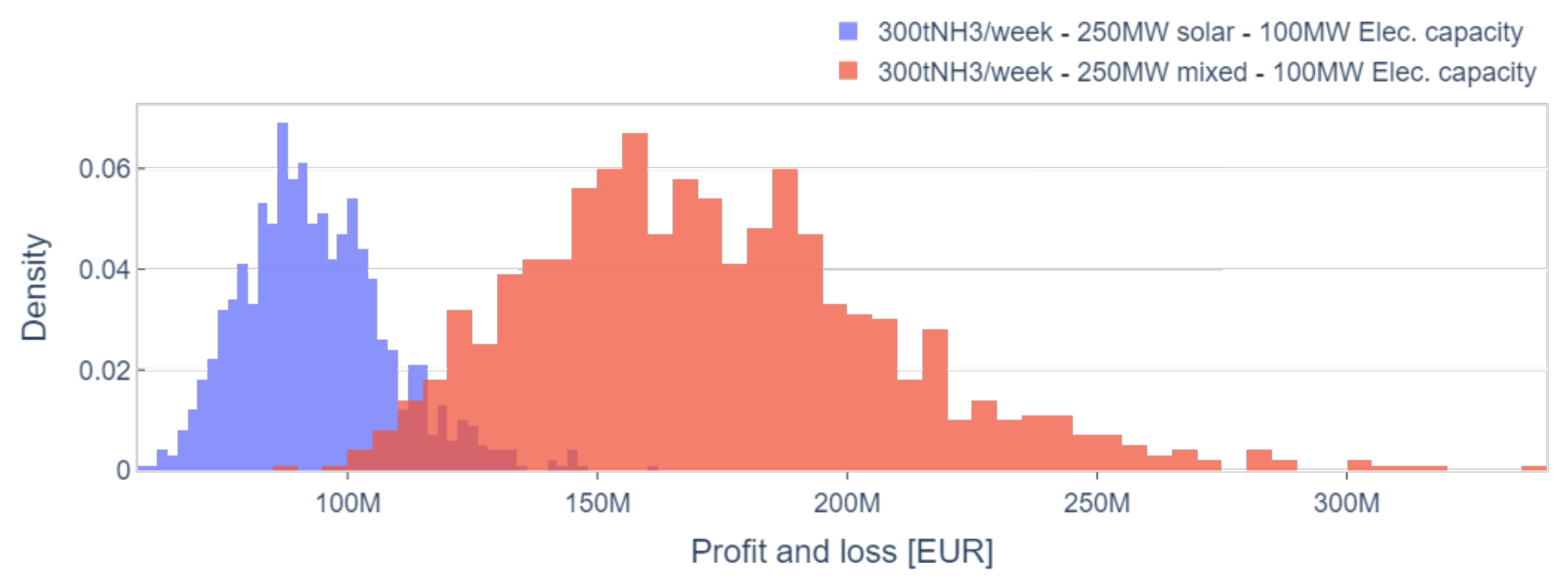
The main outcome of the optimization model is the profit and loss (P&L) distributions generated by each scenario. The median (also referred to as P50) of each distribution is used as a proxy for the midpoint outcome (i.e., the 50th percentile). As some of the distributions are skewed, the median was chosen as opposed to the mean to reduce the weight on extreme values. The standard deviation is shown to quantify the risk, i.e., the higher the standard deviation, the higher the dispersion of the data around the mean and, therefore, the higher the risk around the distribution. Figure 3 illustrates the distributions in the co-located scenario. The blue distribution (i) represents solar generation only, while the red distribution (ii) depicts a 50:50 mix of solar and wind. All other factors, such as NH3 commitment and electrolyzer capacity, remain consistent across both scenarios.
In both cases, the median P&L is positive. Notably, the following observations can be made:
- Solar energy generates less volatile revenues compared to wind energy. Furthermore, the lower load factor and production profile of solar results in a lower median P&L, as the generation is generally lower, and the system is forced to buy external electricity.
- Combining wind and solar power reduces the risk of cannibalization, therefore maximizing profit optimization activities for the electrolyzer but increasing volatility.
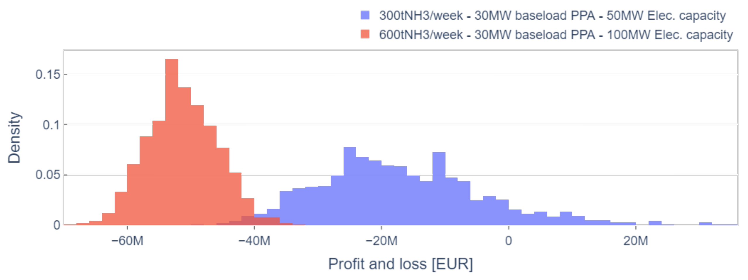
Figure 4 illustrates the BL case and depicts two distributions. The red distribution (iii) corresponds to a commitment of 600 t/week NH3 and an electrolyzer capacity of 100 MW. The blue distribution (iv) represents a commitment of 300 t/week NH3 and a 50 MW electrolyzer. In both cases, the electricity capacity procured via the BL PPA is 30 MW, which results, on average, in a similar amount of energy procured via the PaP PPA. As shown in Table 1, buying a BL PPA is more expensive than the PaP alternative since, in this case, the profile and volumetric risk are removed.
The P&L in both scenarios (iii) and (iv) is adversely affected by the higher price/lower volume of electricity procured via the BL PPA, resulting in a higher probability of incurring losses over the three-year period under consideration. In Scenario (iii), there is less variability but lower median values. Scenario (iv) exhibits improved median values (though still negative) but at the cost of significantly higher variance.
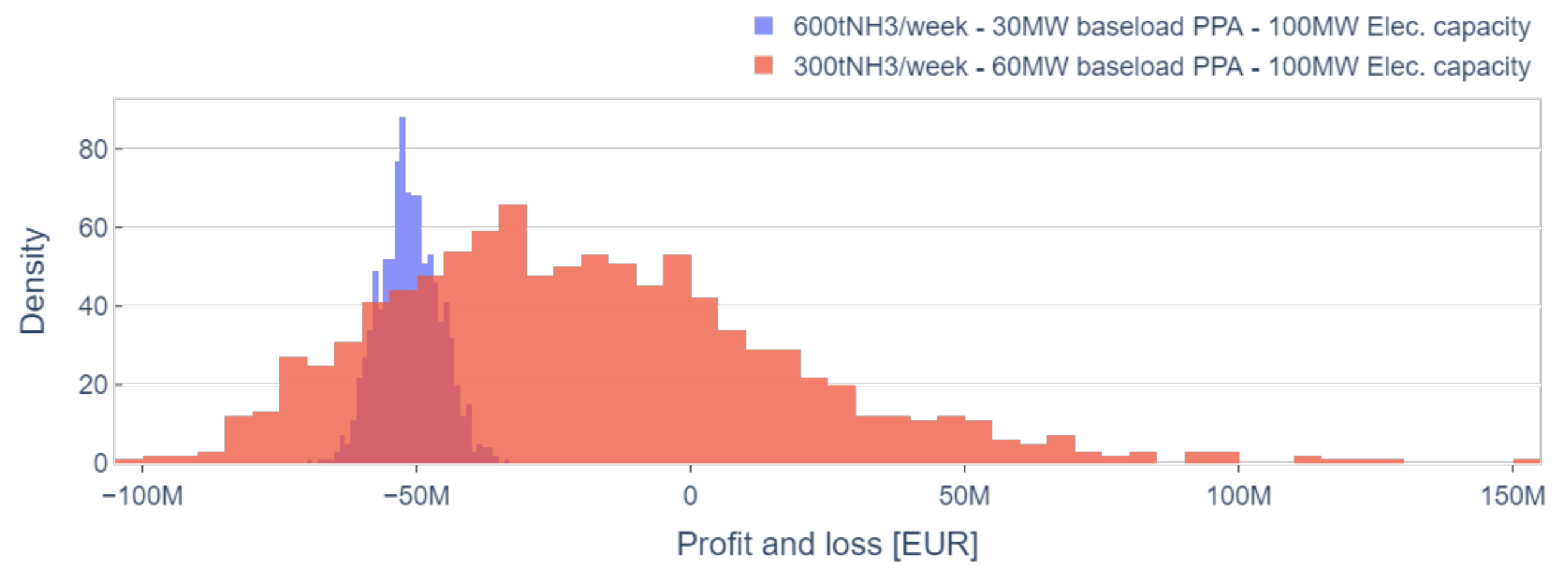
In Figure 5, we examine the same BL configuration but with a fixed electrolyzer capacity of 100 MW. The red distribution (v) showcases the scenario with a delivery commitment of 300 t/week NH3 and a 60 MW Baseload PPA, where we want to test what happens when more energy is secured via a PPA. We compare this to Scenario (iii) from above, in blue in Figure 5, which results from a delivery commitment of 600 t/week of NH3 and a 30 MW BL PPA.
From Scenario (v), the benefit of fixing the price for a larger volume of electricity is clear, resulting in a better median P&L.
Analyzing the BL case and findings (iii), (iv), and (v), the following conclusions can be drawn:
- Increased committed volumes of NH3 reduce revenues’ uncertainty, resulting in a lower P&L volatility but also lower median P&L.
- In a high-price environment, more energy through a BL PPA results in an improved median P&L, as it fixes the electricity price throughout the entire duration of the contract, thus significantly reducing price risk.
- However, we can see that a BL PPA generally hampers the system performance by restricting opportunities for profit optimization and NH3 production in the electricity market.
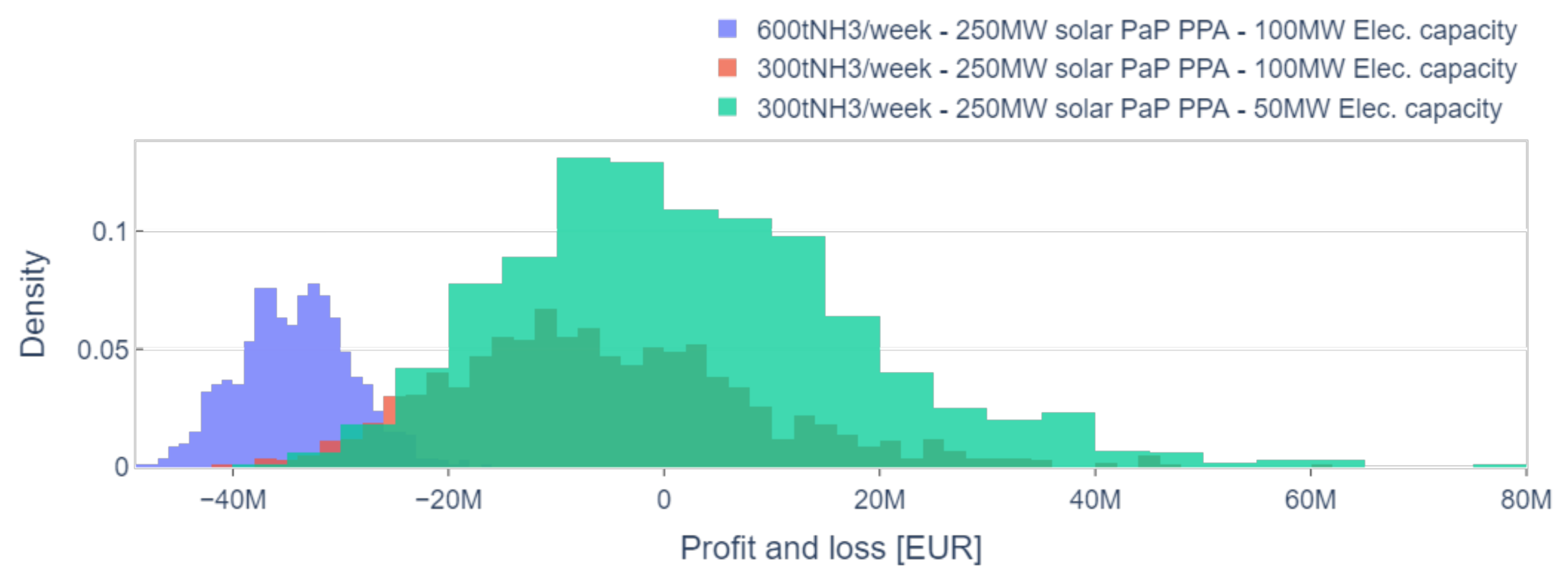
Solar PPA (250 MW) scenarios are depicted in Figure 6, illustrating various configurations. The blue distribution (vi) considers a weekly contract of 600 t of NH3 along with a 100 MW electrolyzer. In the red distribution (vii), a weekly contract of 300 t of NH3 is paired with a 100 MW electrolyzer. Lastly, the green distribution (viii) represents the case where a 300 t of NH3 contract per week is combined with a 50 MW electrolyzer.
The findings from Case (vi) further support the fact that increasing the quantity of NH3, coupled with a higher electrolyzer capacity, enhances predictability but limits the potential to capitalize on higher electricity sale prices, therefore negatively impacting the P&L. In contrast, Cases (vii) and (viii) show more volatile outcomes while exhibiting an overall improvement in terms of median P&L. By reducing the electrolyzer capacity in Case (vii), flexibility is reduced, leading to fewer opportunities to optimize NH3 production. However, this approach enables higher profits through the sale of electricity during peak hours as a result of solar generation. It is important to note that relying solely on a solar profile may not maximize the P&L from electricity sales, as the solar generation profile typically aligns closely with consumption patterns, resulting in limited opportunities to buy electricity during off-peak hours (usually at night) and sell it during peak periods.
In summary, in the case of a Solar PPA, it can be concluded that:
- Solar generation input enhances the P&L for electricity when compared to BL generation. However, there is still room for improvement based on the interplay between the solar profile and consumption patterns.
- Confirming the findings of the BL case, higher committed NH3 volumes, and increased electrolyzer capacity contribute to a reduction in volatility. However, these factors still have a negative impact on the P&L.
- Optimal P&L for solar is achieved by adopting lower NH3 commitments and a smaller electrolyzer capacity. This outcome can be attributed to the higher value of electricity relative to NH3, which is likely influenced by a lower procurement price. When buyers opt for a Pay-as-Produced approach, they receive a discount but also assume the risk of cannibalization associated with the solar profile. The ability to mitigate cannibalization risk using the electrolyzer as a form of storage (i.e., producing ammonia when market electricity prices are low) further supports the superior P&L of this configuration.
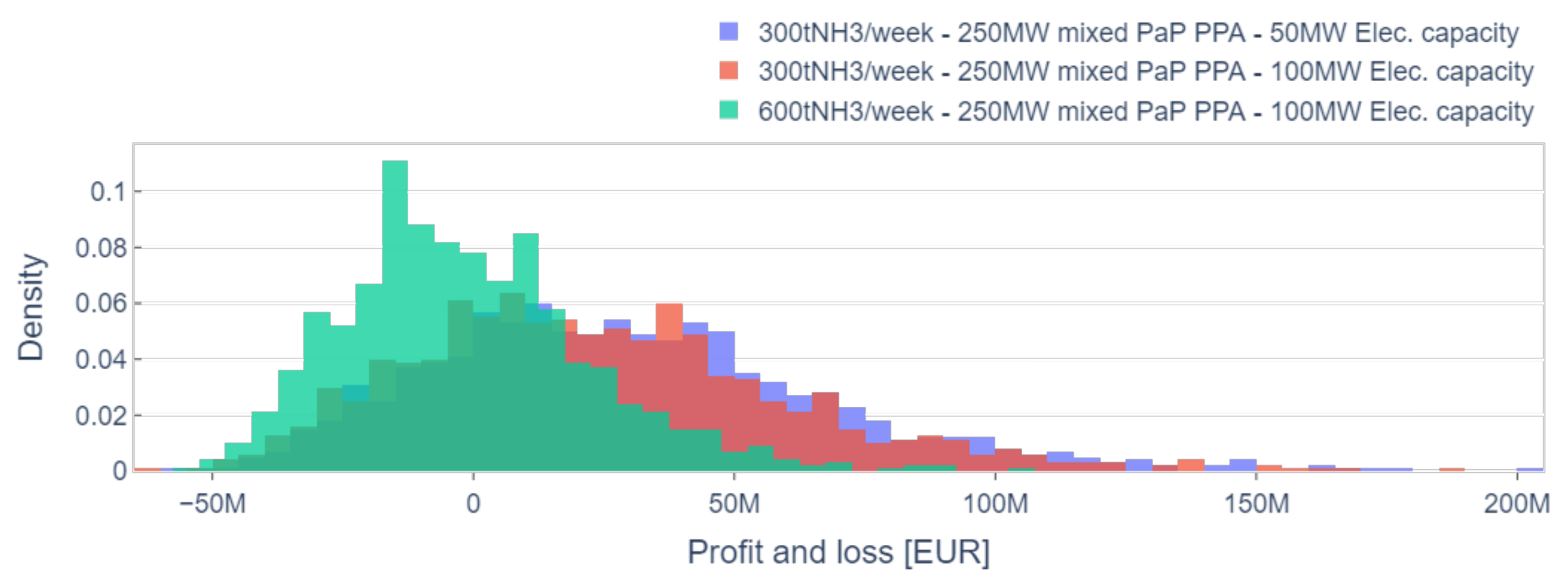
To investigate the potential benefits of a mixed generation profile, the next case incorporates wind generation to determine if such a combination enhances the ability to store electricity during off-peak periods and maximize sales during peak hours. Figure 7 illustrates scenarios of mixed solar and wind PPA with capacities of 125 MW each and Pay-as-Produced generation. The blue distribution (ix) represents a scenario with a weekly contract for 300 t of NH3 and an electrolyzer capacity of 50 MW. The red distribution (x) corresponds to a scenario with the same weekly NH3 contract but with an electrolyzer capacity of 100 MW. Lastly, the green distribution (xi) depicts a scenario with a weekly NH3 contract of 600 t and an electrolyzer capacity of 100 MW.
All three cases show a significant improvement compared to the BL, PaP, and Solar cases. As expected, buying in equal parts a wind and solar profile results in lower cannibalization risk (while still enjoying a lower PPA electricity cost), thus allowing the electrolyzer activity to be focused on optimizing between electricity and NH3 sale. Selling electricity is more profitable than selling NH3 in the recent high-price environment, particularly when obtained at a discount through a PaP PPA. This idea is further reinforced in the case of wind and solar, where cannibalization risk is mitigated by the negative correlation between the two generation profiles. Furthermore, it is worth emphasizing that when in activity, the electrolyzer has a minimum load of 20% of its capacity. As a result, the higher the capacity of the electrolyzer, the larger the minimum amount of electricity for operation, leaving less room for optimization. All three cases show positive median P&L and higher volatility from a volatile wind production pattern.
Using stochastic prices to optimize a PtX system that produces NH3, we have observed that the most profitable option consists of:
- Procuring the electricity via a Pay-as-Produced PPA featuring a mix of solar and wind generation. This allows one to buy electricity at a discount while minimizing the cannibalization risk, thanks to the negative correlation between wind and solar generation. The mixed input generation profile also allows great optimization, as the electrolyzer has more opportunities to choose from when to produce NH3.
- Committing lower volumes of NH3. We have observed that higher NH3 volume commitment results in lower volatility of the P&L but with a negative impact on the P&L distribution.
- Lower electrolyzer capacity. In the cases analyzed, the result was a higher median profit, as the electrolyzer improved profits by optimizing between the cheap electricity purchased via the PPA and the market prices.
When possible, however, the co-located configuration should be prioritized, possibly with a mixed wind and solar generation, as this choice shows the best outcomes in terms of P&L.
5. Conclusions
This paper has investigated the profitability of producing green ammonia through water electrolysis at a time when green ammonia is becoming a critical tool for decarbonizing the transport and agricultural industries. The required electricity is sourced from renewable energy, utilizing various types of supply contracts that were chosen to reflect the latest project trends. The use of stochastic electricity and ammonia prices, performed for the first time in this study, ensures that the volatile and intermittent nature of electricity is captured in the modeling of future prices. Notably, the presence of co-located renewable generation emerges as a pivotal contributor, offering electricity at an exceptionally low cost. In instances where a co-located system is impractical, our findings advocate for the efficacy of a Pay-as-Produced PPA. This arrangement, especially when characterized by a blend of wind and solar energy coupled with an electrolyzer designed for enhanced flexibility, proves to be an optimal strategy, maximizing project outcomes.
Flexibility plays a pivotal role in harnessing the advantages of cost-effective ammonia production within the market. In the context of this research, flexibility primarily stems from reduced contractual obligations related to ammonia production. Flexibility can be further achieved through the implementation of battery storage systems. This underscores the critical importance of investing in flexible assets not only to optimize grid performance but also to bolster the economic viability of PtX projects. Renewable electricity prices, ammonia contractual obligations, and the minimum load of the electrolyzer are identified as the key determinants affecting profits. The profitability of the process was limited to the sale of ammonia, but future research aims to expand it to the possible production of green hydrogen.
The significance of this research extends to both policy formulation and strategic investment decisions, offering a versatile framework for evaluating PtX system performance. This framework is instrumental in multiple ways: first, by pinpointing the pivotal parameters influencing a project’s financial success; second, it gauges project risks by quantifying returns volatility; third, it facilitates project financing by establishing a structured approach for forecasting future cash flows and requirements. This will not only bolster access to project funding but also align seamlessly with contemporary decarbonization and renewable energy policies.
Author Contributions
Conceptualization, E.L., A.T. and H.G.; methodology, E.L., A.T. and H.G.; software, E.L. and A.T.; validation, E.L. and A.T.; formal analysis, A.T.; investigation, E.L. and A.T.; resources, E.L. and A.T.; data curation, E.L. and A.T.; writing—original draft preparation, E.L. and A.T.; writing—review and editing, E.L., A.T. and H.G.; visualization, A.T.; project administration, E.L.; supervision, H.G. All authors have read and agreed to the published version of the manuscript.
Funding
This research received no external funding.
Institutional Review Board Statement
Not applicable.
Informed Consent Statement
Not applicable.
Data Availability Statement
The data presented in this study are available on request from the corresponding author.
Conflicts of Interest
The authors declare no conflicts of interest.
Abbreviations
The following abbreviations are used in this manuscript:
| BL | Baseload |
| CFR | Cost&Freight |
| CAPEX | Capital expenditure |
| EEX | European Energy Exchange |
| GBM | Geometric Brownian Motion |
| GW | Gigawatts |
| IEA | International Energy Agency |
| ktonnes | kilo tonnes |
| Mtonnes | Mega tonnes |
| MW | Megawatts |
| MWhr | Megawatts hour |
| OPEX | Operational expenditure |
| OU | Ornstein-Ulenbeck |
| PaP | Pay as Produced |
| P&L | Profit and Loss |
| PPA | Power Purchase Agreement |
| PtX | Power-to-X |
Appendix A
The variables optimized through the optimization process and the parameters that are not optimized but given input to the model are listed in Table A1.

Table A1.
List of parameters and variables for the optimization.
| Parameter | Variables Optimized |
|---|---|
| Electrical losses, | Power sold, |
| Price of electricity provided through the PPA, | Power bought, |
| Spot price of the power modeled, | Power used, |
| Power procured through the PPA, | Ammonia produced, |
| Selling price of NH3, | Power used by the electrolyzer, |
| Minimal production capacity of the NH3 process, | Power used for the water treatment, |
| Maximal hourly capacity of the NH3 process, | Power used by the NH3 process, |
| NH3 contract, | H2 produced, |
| Energy consumption for the electrolyzer, | Binary variable for NH3 production, |
| Energy requirement for the water treatment, | |
| Power consumed by the NH3 process when producing NH3, | |
| Power consumed by the NH3 process when in standby, | |
| Mass balance between NH3 and H2, | |
| Mass balance between H2O and H2, | |
| Grid connection limit, |
References
- European Commission. Annual European Union Greenhouse Gas Inventory 1990–2021 and Inventory Report 2023. Available online: https://www.eea.europa.eu/publications/annual-european-union-greenhouse-gas-2 (accessed on 26 May 2023).
- BloombergNEF. 2023 Spain Power Market Outlook. Solar Rebalances Prices. 2023. [Google Scholar]
- International Energy Agency. Global Hydrogen Review 2022. Available online: https://iea.blob.core.windows.net/assets/c5bc75b1-9e4d-460d-9056-6e8e626a11c4/GlobalHydrogenReview2022.pdf (accessed on 21 August 2023).
- RWE. Hydrogen Pipeline in the North Sea. 2023. Available online: https://www.rwe.com/en/research-and-development/project-plans/hydrogen-pipeline-in-the-north-sea/ (accessed on 17 August 2023).
- RWE. RWE and Equinor Agree on Strategic Partnership for Security of Supply and Decarbonisation. 2023. Available online: https://www.rwe.com/en/press/rwe-ag/2023-01-05-rwe-and-equinor-agree-on-strategic-partnership-for-security-of-supply-and-decarbonisation (accessed on 17 August 2023).
- Saeedmanesh, A.; Mac Kinnon, M.A.; Brouwer, J. Hydrogen is essential for sustainability. Curr. Opin. Electrochem. 2018, 12, 166–181. [Google Scholar] [CrossRef]
- Olabi, A.; Abdelkareem, M.A.; Mahmoud, M.S.; Elsaid, K.; Obaideen, K.; Rezk, H.; Wilberforce, T.; Eisa, T.; Chae, K.J.; Sayed, E.T. Green hydrogen: Pathways, roadmap, and role in achieving sustainable development goals. Process Saf. Environ. 2023, 177, 664–687. [Google Scholar] [CrossRef]
- European Commission. Global Hydrogen Review 2022. Available online: https://www.iea.org/reports/global-hydrogen-review-2022 (accessed on 23 April 2023).
- Sandalow, D.; Aines, R.; Fan, Z.; Friedmann, J.; McCormick, C.; Merz, A.K.; Scown, C. Low-Carbon Ammonia Roadmap, ICEF Innovation Roadmap Project. 2022. Available online: https://www.icef.go.jp/pdf/summary/roadmap/icef2022_roadmap_Low-Carbon_Ammonia.pdf (accessed on 18 August 2023).
- Yao, D.; Tang, C.; Wang, P.; Cheng, H.; Jin, H.; Ding, L.X.; Qiao, S.Z. Electrocatalytic green ammonia production beyond ambient aqueous nitrogen reduction. Chem. Eng. Sci. 2022, 257, 117735. [Google Scholar] [CrossRef]
- World Bank. Volume 1: The Potential of Zero-Carbon Bunker Fuels in Developing Countries. 2021. Available online: https://documents1.worldbank.org/curated/en/110831617996384433/pdf/The-Potential-of-Zero-Carbon-Bunker-Fuels-in-Developing-Countries.pdf (accessed on 28 February 2024).
- Shi, J.; Zhu, Y.; Feng, Y.; Yang, J.; Xia, C. A Prompt Decarbonization Pathway for Shipping: Green Hydrogen, Ammonia, and Methanol Production and Utilization in Marine Engines. Atmosphere 2023, 14, 584. [Google Scholar] [CrossRef]
- IWI. Using Ammonia as Fuel. 2023. Available online: https://www.ihi.co.jp/en/sustainable/environmental/climatechange/ammonia_energy (accessed on 17 August 2023).
- Good Earth Cotton. Good Earth Green Hydrogen and Ammonia (GEGHA) Project. 2023. Available online: https://www.goodearthcotton.com/media/gegha (accessed on 17 August 2023).
- Kim, A.; Kim, H.; Lee, H.; Lee, B.; Lim, H. Comparative Economic Optimization for an Overseas Hydrogen Supply Chain Using Mixed-Integer Linear Programming. ACS Sustain. Chem. Eng. 2021, 9, 14249–14262. [Google Scholar] [CrossRef]
- Salmon, N.; Bañares-Alcántara, R. A global, spatially granular techno-economic analysis of offshore green ammonia production. J. Clean. Prod. 2022, 367, 133045. [Google Scholar] [CrossRef]
- Campion, N.; Nami, H.; Swisher, P.; Hendriksen, P.; Münster, M. Techno-economic assessment of green ammonia production with different wind and solar potentials. Renew. Sustain. Energy Rev. 2023, 173, 113057. [Google Scholar] [CrossRef]
- Mays, J. Quasi-Stochastic Electricity Markets. INFORMS J. Optim. 2021, 3, 350–372. [Google Scholar] [CrossRef]
- Leigh, G.J. Haber-Bosch and Other Industrial Processes. In Catalysts for Nitrogen Fixation; Smith, B.E., Richards, R.L., Newton, W.E., Eds.; Springer: Dordrecht, The Netherlands, 2004; pp. 33–54. [Google Scholar]
- Hart, W.E.; Watson, J.P.; Woodruff, D.L. Pyomo: Modeling and solving mathematical programs in Python. Math. Program. Comput. 2011, 3, 219–260. [Google Scholar] [CrossRef]
- Achterberg, T.; Berthold, T.; Koch, T.; Wolter, K. Constraint Integer Programming: A New Approach to Integrate CP and MIP. In Integration of AI and OR Techniques in Constraint Programming for Combinatorial Optimization Problems; Perron, L., Trick, M.A., Eds.; Springer: Berlin/Heidelberg, Germany, 2008; pp. 6–20. [Google Scholar]
- Schwartz, E.S. The Stochastic Behavior of Commodity Prices: Implications for Valuation and Hedging. J. Financ. 1997, 52, 923–972. [Google Scholar] [CrossRef]
- Geman, H. Commodities and Commodity Derivatives: Modeling and Pricing for Agriculturals, Metals and Energy; John Wiley & Sons: Chichester, UK, 2005. [Google Scholar]
- Lucia, J.; Schwartz, E. Electricity prices and power derivatives:Evidence from the Nordic Power Exchange. Rev. Deriv. Res. 2002, 5, 5–50. [Google Scholar] [CrossRef]
- Ross, S. Stochastic Processes; Wiley Series in Probability and Statistics; Wiley: Hoboken, NJ, USA, 1996. [Google Scholar]
- Harvey, A. Forecasting, Structural Time Series Models and the Kalman Filter; Cambridge University Press: Cambridge, UK, 1989; Volume 127. [Google Scholar]
- European Energy Exchange AG. EEX Futures. 2023. Available online: https://www.eex.com/en/market-data/power/futures#%7Bsnippetpicker%3A%2228%22%7D (accessed on 21 August 2023).
- Bloomberg, L.P. United States Rates & Bonds. 2023. Available online: https://www.bloomberg.com/markets/rates-bonds/government-bonds/us (accessed on 21 August 2023).
- Bachelier, L. Théorie de la spéculation. Ann. Sci. L’éCole Norm. SupéRieure 1900, III-17, 21–86. [Google Scholar] [CrossRef]
- Bloomberg, L.P. Western Europe Ammonia CFR 01/01/2020 to 31/01/2023; Retrieved 2023-07-24 from Bloomberg terminal. 2023. [Google Scholar]
- Hank, C.; Sternberg, A.; Köppel, N.; Holst, M.; Smolinka, T.; Schaadt, A.; Hebling, C.; Henning Campbell, H.M. Energy efficiency and economic assessment of imported energy carriers based on renewable electricity. Sustain. Energy Fuels 2020, 4, 2256–2273. [Google Scholar] [CrossRef]
- Statkraft. Fortescue Future Industries and Statkraft Secure Power for Proposed Holmaneset Green Hydrogen and Green Ammonia Project. 2023. Available online: https://www.statkraft.com/newsroom/news-and-stories/2023/fortescue-future-industries-and-statkraft-secure-power-to-holmaneset-project-for-green-hydrogen-and-green-ammonia/ (accessed on 15 November 2023).
- Murchison Hydrogen Renewables Project. 2023. Available online: https://www.murchisonrenewables.com.au/ (accessed on 21 November 2023).
- Iverson. Available online: https://www.iverson-efuels.no/en/ (accessed on 21 November 2023).
- InterContinental Energy. InterContinental Energy Portfolio. 2023. Available online: https://intercontinentalenergy.com/our-portfolio/ (accessed on 15 November 2023).
- HØST PtX Esbjerg. 2023. Available online: https://hoestptxesbjerg.dk/ (accessed on 21 November 2023).
- ENTSOE Transparency Platform. 2023. Available online: https://transparency.entsoe.eu/ (accessed on 22 November 2023).
- TenneT DE. 2023. Available online: https://www.tennet.eu/ (accessed on 22 November 2023).
- Ghiassi-Farrokhfal, Y.; Ketter, W.; Collins, J. Making green power purchase agreements more predictable and reliable for companies. Decis. Support Syst. 2021, 144, 113514. [Google Scholar] [CrossRef]
Figure 1.
Schematic of a Power-to-X plant producing green H2 and green NH3.

Figure 2.
Illustration of the plant configuration where the procurement can be co-located assets, PaP PPA or BL PPA.
Figure 2.
Illustration of the plant configuration where the procurement can be co-located assets, PaP PPA or BL PPA.

Figure 3.
P&L in the case of Co-location, with Scenario (i) in blue and Scenario (ii) in red.

Figure 4.
P&L in the case of BL with different commitment and electrolyzer capacity, with Scenario (iii) in red and Scenario (iv) in blue.
Figure 4.
P&L in the case of BL with different commitment and electrolyzer capacity, with Scenario (iii) in red and Scenario (iv) in blue.

Figure 5.
P&L in the case of BL with a fixed electrolyzer capacity, with Scenario (iii) in blue and Scenario (v) in red.
Figure 5.
P&L in the case of BL with a fixed electrolyzer capacity, with Scenario (iii) in blue and Scenario (v) in red.

Figure 6.
P&L in the case of Solar Electricity, with Scenario (vi) in blue, Scenario (vii) in red, and Scenario (viii) in green.
Figure 6.
P&L in the case of Solar Electricity, with Scenario (vi) in blue, Scenario (vii) in red, and Scenario (viii) in green.

Figure 7.
P&L in the case of mixed Wind and Solar PPA, with Scenario (ix) in blue, Scenario (x) in red, and Scenario (xi) in green.
Figure 7.
P&L in the case of mixed Wind and Solar PPA, with Scenario (ix) in blue, Scenario (x) in red, and Scenario (xi) in green.

Table 1.
Input parameters used in the production model.
| Parameter | Unit | Symbol | Value |
|---|---|---|---|
| Electrical losses | % | 3.0 | |
| Energy requirement for the water treatment | MWh/tH2O | 0.002 | |
| Energy requirement for the electrolyzer | MWh/tH2 | 53.4 | |
| Grid connection limit | MW | 280 | |
| Capacity of the electrolyzer | MW | 100 | |
| Capacity of the Haber–Bosch unit | tNH3/h | 13 | |
| NH3 annual contract | tNH3/week | 600 | |
| Power consumption of the Haber–Bosch unit in operation mode | - | 0.52 | |
| Power consumption of the Haber–Bosch unit in standby mode | - | 0.1755 | |
| Solar installed capacity 1 | MW | 250 | |
| Mixed installed capacity 2 | MW | 250 | |
| PPA baseload price | EUR/MWh | 130.61 | |
| PPA solar PaP price | EUR/MWh | 102.91 | |
| PPA mixed PaP price | EUR/MWh | 100.39 |
1 Value used for the co-located configuration and the Pay-as-Produce Solar PPA. 2 Value used for the co-located configuration and the Pay-as-Produce Mixed PPA (125 MW solar, 125 MW onshore wind).
Table 2.
Data sources, description and reference for the datasets used in the model.
| Data | Source | Description | Reference |
|---|---|---|---|
| Wind production | Co-located | Historical wind production for 2020 in Germany | [37,38] |
| Solar production | Co-located | Historical solar production for 2020 in Germany | [37,38] |
| Forward electricity settlement prices | European Power Exchange | Daily closing settlement prices for the forward contracts M1, Q1, Y1, Y2 and Y3 | [27] |
| Spot price for ammonia | Western Europe Ammonia CFR (Cost&Freight) | Historical spot price for ammonia from 1 January 2020 to 31 January 2023 | [30] |
Table 3.
Detailed list of scenarios, where the procurement configuration, the technology of the renewables providing the electricity, the capacity of the electricity contract, the capacity of the electrolyzer, the size of the weekly ammonia contract, the median (P50) of the P&L distribution and the standard deviation of the P&L distribution are shown for each scenario.
| Scenario | Procurement | Technology | Renewable Capacity [MW] | Electrolyzer Capacity [MW] | NH3 Contract [t/Week] | P50 P&L M€ | Std P&L M€ |
|---|---|---|---|---|---|---|---|
| i | Co-located | Solar | 250 | 100 | 300 | 92 | 15 |
| ii | Co-located | Mixed | 250 | 100 | 300 | 169 | 37 |
| iii | BL | - | 30 | 100 | 600 | −52 | 5.5 |
| iv | BL | - | 30 | 50 | 300 | −18 | 13 |
| v | BL | - | 60 | 100 | 300 | −22 | 37 |
| vi | PaP | Solar | 250 | 100 | 600 | −34 | 5 |
| vii | PaP | Solar | 250 | 100 | 300 | −7 | 15 |
| viii | PaP | Solar | 250 | 50 | 300 | 0.3 | 17 |
| ix | PaP | Mixed | 250 | 50 | 300 | 26 | 38 |
| x | PaP | Mixed | 250 | 100 | 300 | 20 | 37 |
| xi | PaP | Mixed | 250 | 100 | 600 | −4 | 23 |
Disclaimer/Publisher’s Note: The statements, opinions and data contained in all publications are solely those of the individual author(s) and contributor(s) and not of MDPI and/or the editor(s). MDPI and/or the editor(s) disclaim responsibility for any injury to people or property resulting from any ideas, methods, instructions or products referred to in the content. |
© 2024 by the authors. Licensee MDPI, Basel, Switzerland. This article is an open access article distributed under the terms and conditions of the Creative Commons Attribution (CC BY) license (https://creativecommons.org/licenses/by/4.0/).
Share and Cite
MDPI and ACS Style
Lauro, E.; Têtu, A.; Geman, H. Green Ammonia Production in Stochastic Power Markets. Commodities 2024, 3, 98-114. https://doi.org/10.3390/commodities3010007
AMA Style
Lauro E, Têtu A, Geman H. Green Ammonia Production in Stochastic Power Markets. Commodities. 2024; 3(1):98-114. https://doi.org/10.3390/commodities3010007
Chicago/Turabian StyleLauro, Ezio, Amélie Têtu, and Hélyette Geman. 2024. "Green Ammonia Production in Stochastic Power Markets" Commodities 3, no. 1: 98-114. https://doi.org/10.3390/commodities3010007