
Trading Behavior in Agricultural Commodity Futures around the 52-Week High


UWA Business School, University of Western Australia, Perth, WA 6009, Australia
Commodities 2022, 1(1), 3-17; https://doi.org/10.3390/commodities1010002
Submission received: 27 April 2022
/
Revised: 16 June 2022
/
Accepted: 17 June 2022
/
Published: 21 June 2022
Abstract
:Utilizing the Commodity Futures Trading Commission’s Commitment of Traders report, we examine the behavior of traders in three large agricultural futures markets (corn, soybean, and wheat) when prices are at a key technical trading level—the 52-week high (the highest price during the past year). Our empirical results confirm that, consistent with hedging behavior, commercial traders tend to be negative feedback traders, while non-commercial traders tend to be momentum traders. In both cases, there is a moderating effect when the market is at the 52-week high. For non-commercial traders, this effect is concentrated in short positions. Although we find no evidence of a broad market timing ability from any trader type, trader positions appear to be more informative when the market is at the 52-week high. Our results have implications for traders attempting to time market entry.
Keywords:
futures markets; trading behavior; CFTC COT; market timing; momentum; agricultural futures1. Introduction
Futures contracts on agricultural commodities are one of the earliest financial innovations. First introduced in ancient Mesopotamia, they have allowed farmers, and other producers, to hedge price risk for millennia [1,2]. In the modern era, grain futures were the first contracts traded upon the foundation of the Chicago Board of Trade (CBOT) in 1848 (Available online: https://www.cftc.gov/About/HistoryoftheCFTC/history_precftc.html; accessed on 1 April 2022). Nowadays, commodity markets offer diversification benefits to traditional stock and bond portfolios and the potential of an inflation hedge. As a result, commodity markets have experienced a dramatic expansion in investor interest over the past few decades. Financialization has facilitated investor access to these markets via a variety of investment vehicles, with futures markets playing a key role. Their increasing importance, particularly as investors seek a means to protect against rising global prices, suggests it is worthwhile gaining further insight into trading behavior within these markets.
We utilize the weekly Commitment of Traders (COT) report issued by the Commodity Futures Trading Commission (CFTC) to understand the determinants of trading behavior, and market timing ability, in the futures markets for three crops: corn, soybean, and wheat. While several prior studies have utilized the COT report, there remains disagreement as to how traders respond to price changes and whether traders exhibit market timing ability. In revisiting this topic for an updated sample period, we contribute to the empirical argument. In addition, we consider how trader positions evolve around a key technical trading signal—the 52-week high. This issue has yet to be examined in the literature and is especially important given the prevalence of Commodity Trading Advisors (CTAs) that utilize momentum trading strategies within futures markets [3].
The first question we tackle relates to position changes of different trader types in response to market returns. Ref. [4] document considerable differences in the type, size, and turnover of positions for different traders. They note that it is sometimes difficult to classify traders according to the terms of hedgers and speculators since hedgers may engage in speculation (by choosing to over- or under-hedge), and speculators may act as hedgers (by hedging positions in related markets). It may also be beneficial for speculators to misclassify themselves in order to access the larger position limits open to hedgers.
There is substantial evidence that traders respond to price changes [5,6,7] across a range of markets. Ex ante, the response of both commercial traders (hedgers) and non-commercial traders (speculators) is unclear. Intuitively, one might expect that commercial traders would sell when prices rise to lock in higher prices for their products. This relates to the Keynes–Hicks argument whereby hedgers use futures markets to avoid risk and pay speculators for the privilege, creating hedging pressure on prices in doing so [8]. However, [9] show that this hedging pressure offers only a partial explanation of profits observed from momentum strategies based on the 52-week high. It is also possible that hedging is selective based on market outlook, which may be an attempt to exploit the informational advantages of local conditions [10,11].
Similarly, there are opposing arguments for the response of speculators to price changes [12]. On the one hand, it is possible that speculators are momentum traders who destabilize markets by pushing prices away from fundamental values. On the other hand, speculators would effectively be contrarian traders under the speculative stabilizing theory [13] who profit by buying when the price is low and selling when the price is high.
Empirical evidence most commonly finds that commercial traders (hedgers) are contrarian, or negative feedback, traders who sell futures when prices increase and vice-versa. In contrast, non-commercial traders (speculators) are found to be positive feedback or momentum traders [5,14,15,16]. However, the question is not completely resolved since [17,18] found that hedgers engage in positive feedback trading. The positions of commercial traders appear to have a destabilizing impact on futures markets, while speculator positions help to reduce volatility [12,17,18,19]. Relatedly, there is evidence that short-term position changes are motivated by the liquidity demands of speculators [11,20], while long-term adjustments result from the hedging demands of commercial traders.
The second question we focus on is whether there is evidence of market timing ability among either commercial or non-commercial traders. The existing empirical studies have produced mixed results. For instance, although there is a positive contemporaneous correlation between speculator positions and returns [12,21,22], several authors report that positions do not lead, or predict, returns in a variety of future markets [5,6,14,23]. Others find that speculators provide valuable timing indicators in agricultural futures [24], currency futures [25], financial futures [26], and even Bitcoin futures [27]. There is even evidence of superior forecasting ability among speculators in frozen pork bellies futures [28] and S&P 500 index futures [17,29].
As stated earlier, we contribute to the discussion surrounding these questions by focusing on trading behavior when the market is at the 52-week high. In addition to the importance of this technical signal for momentum traders, such as CTAs, this is a potentially interesting signal for commercial traders. As mentioned, they could take advantage of elevated market prices to lock in high product prices by selling more contracts, or if they have believed there is a possibility of a technical breakout (or have insight into future prices), then they would lower their hedging ratio.
Momentum trading strategies are known to be highly profitable in commodity futures markets [30,31]. Ref. [32] demonstrate that a strategy based around the 52-week high explains most of the profits from momentum investing, and this generates profits across international markets [33,34]. Ref. [35] suggest that the strategy’s profitability is linked to investor sentiment. Ref. [32] explain that this behavior results from traders using the 52-week high as a reference point against which news is evaluated. Ref. [36] show that this influences trading decisions, and so volume is substantially higher around the 52-week high.
An example of the type of trading behavior we examine occurs at the end of February 2022, as Russian armed forces gathered on the Ukrainian border. At this time, the price of wheat futures hit a 52-week high above 1000 cents (USD 10). Accompanied by a jump in trading volume, the net positions of commercial traders went from long to short within two weeks, and non-commercial traders flipped from net short to net long within one week.
To summarize, we focus our attention on two related research questions. First, do trader positions respond to market returns? Second, are trading positions informative in futures markets for agricultural commodities? In both cases, we then seek to determine whether the response changes when prices are at the 52-week high.
2. Data and Methods
2.1. Futures Prices and Returns
We focus on the three most actively traded agricultural futures on the Chicago Board of Trade (CBOT), which is part of the Chicago Mercantile Exchange (CME) group: Corn, Soybean, and Wheat. Each of these contracts require physical delivery upon expiry, has a contract size of 5000 bushels, and is priced in U.S. cents per bushel. Prior to January 1998, the contract size was 1000 bushels—we adjusted our data to reflect this and ensured measured units were consistent throughout our sample period. Since the 2012 acquisition of the Kansas City Board of Trade, the CME group has offered futures in both Hard Red Winter (HRW) and Soft Red Winter (SRW) wheat futures. Although the US production of HRW wheat is larger than that of SRW [37], we focused on SRW wheat futures since they have substantially higher trading volume and open interest.
Futures price data were obtained from DataStream for the period from January 1993 to March 2022. Weekly log returns (rt = log (rt/rt1)) were computed to line up with the trader position data. We followed standard practice in using a roll-over strategy so that the most liquid contract was used to compute returns, with the switch typically occurring in the delivery month.
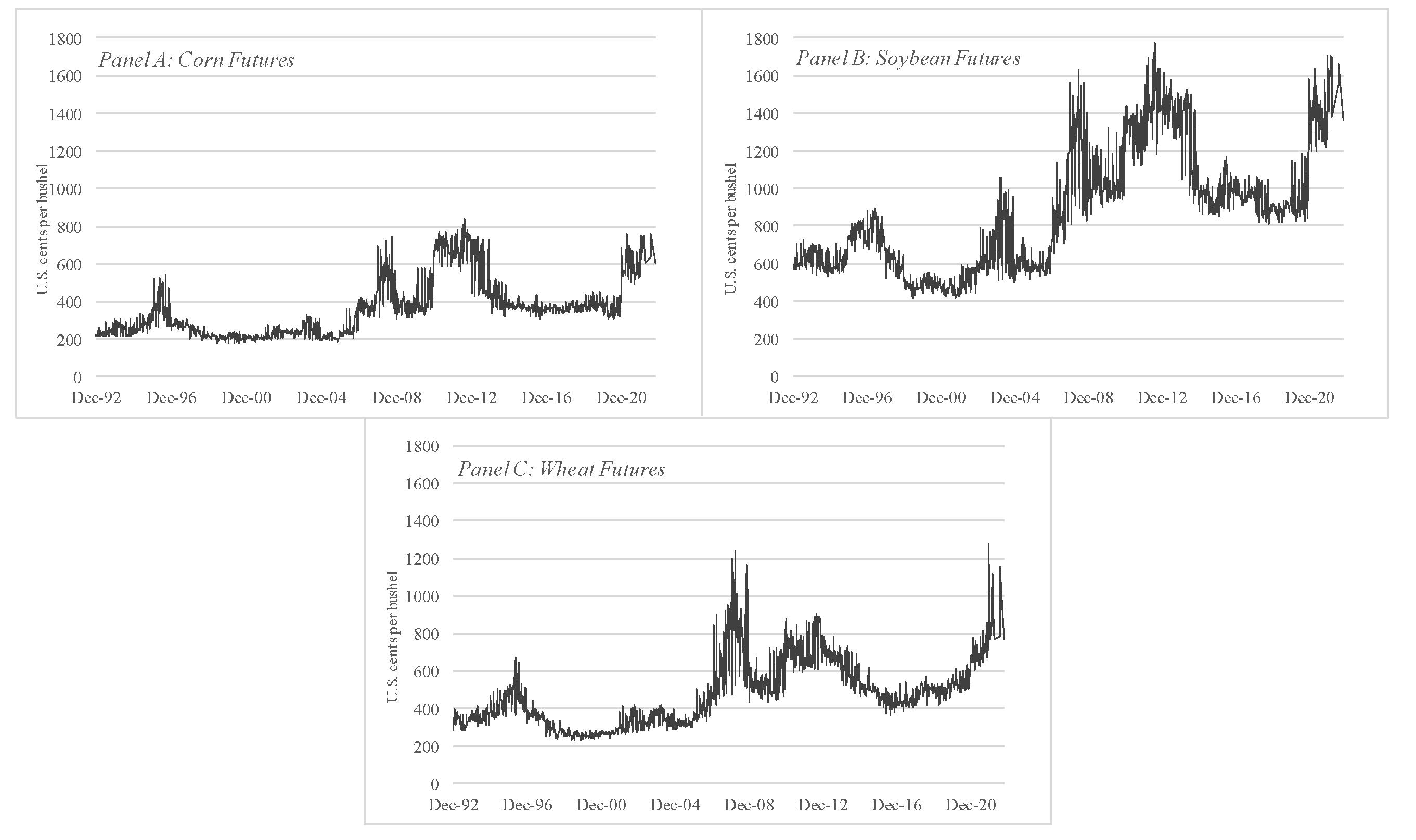
The daily closing price for each futures contract during our sample period is shown in Figure 1. The patterns are similar for all three crops, with sharp price increases in 1996 (more pronounced for corn, less for soybean), 2008, 2011–2012 (less pronounced for wheat), and 2021–2022. The latter surge was driven by recovery from the COVID-19 pandemic, associated shortages in fertilizer, and exacerbated by the Russian invasion of Ukraine (both major exporters of grains).
Panel A of Table 1 provides descriptive statistics for futures returns for the entire sample period. Corn futures have a slightly higher average weekly return (0.079%) than Soymeal (0.069%) or Wheat (0.070%) futures. Corn futures have the largest weekly drawdown (−32.8%), but wheat futures returns are more volatile on average. All weekly returns exhibit fat-tails (kurtosis), which are common within the time-series of financial assets.
2.2. Trader Positions
Trader position information was accessed via the U.S. Commodity Futures Trading (CFTC) Commitment of Traders (COT) report that is published weekly. We focused on the ‘legacy report’ classifications, which classifies traders as commercial or non-commercial, with all reportable traders required to report their open futures positions as of each Tuesday. Commercial traders include producers, merchants, processors, and users of the commodity. It may be possible to glean additional information by disaggregation of the non-commercial positions as per the ‘supplemental report’ or ‘disaggregated report’, but our main focus was on the trading behavior of commercial traders, and so there is little benefit from doing so. Note that the ‘supplemental report’ adds index traders as a third classification. The ‘disaggregated report’ classifies non-commercial traders as swap dealers, managed money, and ‘other reportables’.
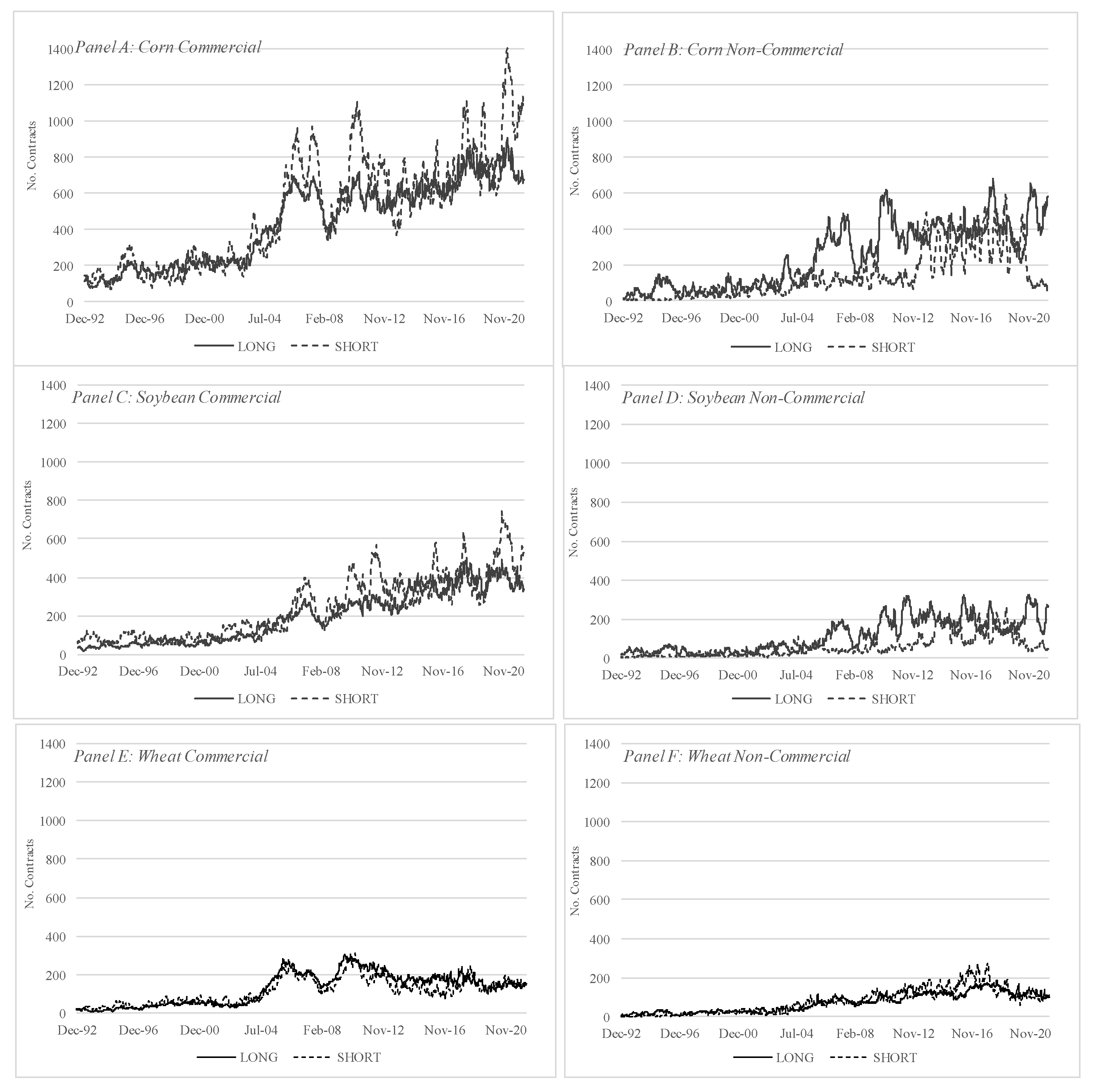
The COT report provides the long, short, and spread positions for each trader type. Figure 2 shows the long (longkt) and short (shortkt) positions of each trader type k in week t. Focusing on commercial traders first, we saw similar patterns in corn and soybean futures. Through the sample period, there was an increase in both long and short positions, with notable spikes in long positions in 2008, 2011–2012, 2018, and 2021. Three of those periods coincided with the sharp price increases shown in Figure 1. Although the commercial positions in wheat futures have also increased over time, there were less noticeable spikes in long (or short) positions. Non-commercial trader positions also seem to have increased over time in all three futures markets; there seems to be significantly more position volatility, and a noticeable spike in wheat futures short positions during 2017.
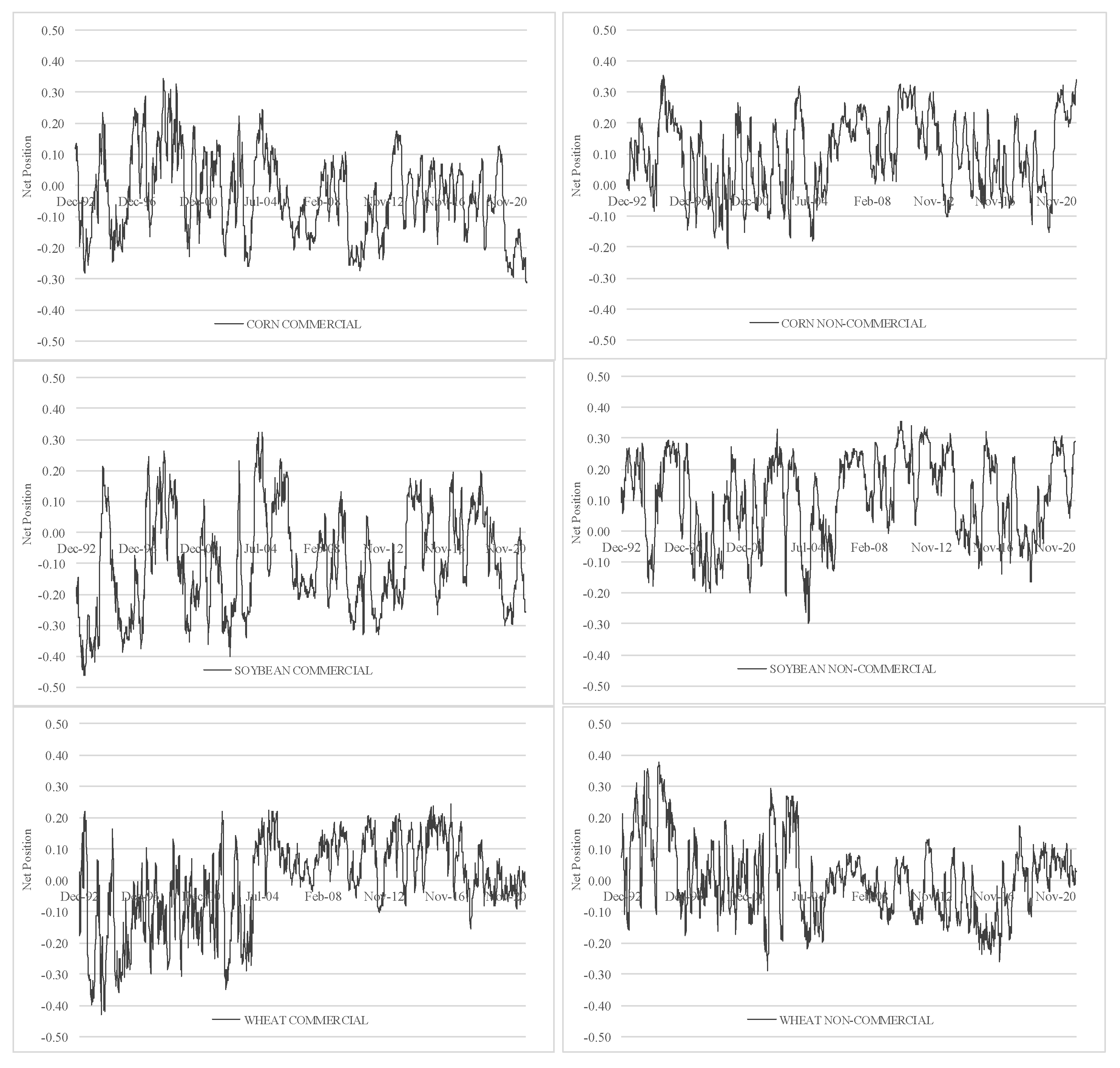
We use the long and short positions of each trader type to compute a measure of net trader position (NPkt) for each trader type k in week t. This is scaled by total open interest (OIt) to control for variation in market size over time.
Table 1 shows that commercial positions tend to be net short on average (only just for wheat futures). This makes sense if one presumes that commercial traders tend to be producers who are long the underlying crop and are using futures to hedge this position. Weekly changes (first differences) are very close to zero, negatively skewed, and leptokurtic. Conversely, non-commercial tend to be net long on average, with positively skewed and leptokurtic weekly changes. The net positions do not sum to zero because we do not consider positions of ‘other reportable’ or ‘other non-reportable’ positions. We do not consider this trader type because of their relatively small size and their herding behavior with large non-commercial traders [15], suggesting limited benefits from additional analysis.
Panel B of Table 1 provides summary information for net positions when each futures market is trading at the 52-week high. When this occurs, the net positions of commercial (non-commercial) traders are significantly lower (higher) than average, and weekly changes are significantly more negative (positive) than average. That is, commercial traders tend to be shortest when prices are at 52-week highs, an indication that commercial traders have increased their hedge as prices increase. When considering 52-week lows, we do not find any significant difference from the mean in net positions.
Figure 3 shows how the net positions of each trader type have changed in each market over time. The net position of commercial traders in wheat futures tends to be more negative at the start of the sample, and then more positive post-2004, with the opposite feature present in non-commercial positions.
3. Empirical Analysis and Discussion
3.1. Trader Positions at the 52-Week High
We consider how different trader types respond to changes in market conditions using a methodology that is similar to [18]. We augment the model by including a dummy variable (HI52) that indicates whether the market is trading at a 52-week high and an interaction term between the dummy variable and market returns. The ordinary least squares (OLS) regression is specified:
where ΔNPkt is the change in net position for trader type k in week t. Rt−1 is the relevant futures return in the prior week, and HI52 is the dummy variable indicating a 52-week high. Φ refers to a set of economic control variables that includes the weekly change in VIX, the 3-month T-Bill yield (TBILL), the Baa-Aaa credit spread (CRDSPRD), and the difference between 10-year and 2-year government securities proxies for the term structure (TERM). The lagged dependent variable is included to account for serial correlation in net position changes. ε is the error term.
The estimated results are reported in Table 2 with the Newey–West standard errors in parentheses. The results are reported separately for corn (Panel A), soybeans (Panel B), and wheat (Panel C) futures, but the inferences are the same across markets.
Prior to consideration of the 52-week high (i.e., the first column for each commodity), the net positions of commercial traders respond negatively to returns in all cases—they become less positive or more negative when prices increase. This contrarian trading is consistent with the hedging behavior of commercial traders identified by [5,14]. When we consider the relevance of the 52-week high (i.e., the second column for each commodity), we again see evidence of contrarian trading in the lagged return coefficient (Rt−1), while the HI52 dummy variable is not statistically significant. However, the interaction term (HI52 × Rt−1) is significant and opposite to the sign for Rt−1, indicating a moderating effect when the market is at a 52-week high. Net positions of commercial traders still become more negative when prices rise past the 52-week high, but the pace slows (for example, the net effect for corn futures is −0.379 + 0.255 = −0.124). In other words, commercial traders temper their hedging behavior when the market makes new highs. This is somewhat surprising, as we might expect that commercial traders would be enticed to hedge more when market prices are elevated to lock in high prices for their products but could be due to traders holding insights into future price movements.
In contrast, non-commercial traders have net positions that are positively related to returns. Non-commercial traders seem to be momentum traders who increase their net long position (or reduce net shorts) when prices increase. Again, there is a moderating effect at the 52-week high whereby the net position change is lower than otherwise (for example, the net effect for corn futures is +0.360 − 0.271 = 0.089). The control variables have no significant impact on trader positions in any of the markets considered.
We provide supporting evidence for our results in Table 3. We conduct a set of pairwise Granger Causality tests using bivariate regressions of the form:
The number of lags was set to five (l = 5) based on the optimal Akaike information criterion (AIC) and Schwarz information criterion (SIC). The pairwise Granger Causality tests failed to reject the null hypothesis of returns not causing changes in net positions across all three markets and for both trader types. In other words, consistent with the significant return coefficient shown in Table 2, futures Granger returns cause net position changes for both commercial and non-commercial traders in all three markets. In addition, there is evidence that changes in non-commercial positions are caused by changes in commercial positions for corn and soybean markets. This is consistent with the hedging demands of commercial traders driving position variations (as in [11]). The converse is true for the wheat market, with non-commercial traders Granger causing net position changes. This difference could be due to the relative power of producers in each market or the relative liquidity needs of participants in each market (with net positions/liquidity requirements in the wheat market very close to zero on average).
As our initial analysis focused on net positions, a related question is whether both long and short positions respond to returns. Table 4 shows that returns do indeed seem to be significantly related to long and short position changes. For all three markets, a positive return is associated with a decrease in long positions, and an increase in short positions of commercial traders. This result provides further evidence of hedging behavior among commercial traders. Similarly, there is more evidence of momentum trading among non-commercial traders who increase longs, and decrease shorts, when returns are positive. The moderating influence of the 52-week high on net position changes seems to apply to both long and short commercial positions; it seems to be concentrated in short positions for non-commercial traders across all markets. In addition, non-commercial position sizes are negatively related to credit spreads. One reason could be that speculators use trading strategies that require access to margin credit and so are forced to decrease their position size when credit costs increase (or credit availability declines).
3.2. Market Timing
We identified that trader positions respond to market returns, and while we have some evidence (Table 3) that position changes do not cause returns, this does not necessarily mean that knowledge of trader positions is not useful in predicting returns. In this section, we use the method of [22] to examine whether returns may be predicted from changes in trader positions after controlling for the prevailing position level. The OLS model is:
where Rt is the relevant futures return in week t. NPkt and ΔNPkt are the level and change in net position for trader type k in the prior week (t−1). HI52 is a dummy variable indicating a 52-week high. Φ refers to a set of economic control variables that includes the weekly change in VIX, the 3-month T-Bill yield (TBILL), the Baa-Aaa credit spread (CRDSPRD), and the difference between 10-year and 2-year government securities proxies for the term structure (TERM). ε is the error term.
Table 5 shows that, in general, there is very little evidence that any trader type has market timing ability within the agricultural futures market. This is contrary to [24,28] but consistent with [5,14,23]. Panel A shows that the only statistically significant indicator is the change in the net position of non-commercial traders within the soybean market. Panel B disaggregates net positions into long and short positions, which [7] suggests may provide a more accurate picture of the economic positioning of each trader type. There remains little consistent evidence of any timing ability. The long positions of commercial traders have some relevance in corn and wheat markets, but their short positions are relevant in the soybean market. None of the non-commercial positions have a statistically significant relationship with returns. Essentially, this analysis confirms the results presented in Table 3 such that position changes do not cause (predict) Granger returns.
Earlier, we identified that when the crop futures markets reach a 52-week high, there is a moderating effect on hedging behavior. It is possible that this effect is related to market timing ability during such periods. We test this by repeating our regression estimates for Equation (4) but focusing only on the periods when the market reaches a 52-week high. Panel A of Table 6 shows that changes in trader positions (corn) and prevailing levels of trader positions (soybean and wheat) are much more informative when the market is at a 52-week high. There is an interesting dichotomy between markets as the estimated commercial net position level (NP) coefficient is negative for soybean but positive for wheat (and corn). This suggests that shorter commercial net positions predict positive (negative) next period returns in soybean (wheat) futures markets when the market is at highs. The next period return for soybean futures is predicted to be positive (+) since a negative short position (−) is multiplied by a negative estimated coefficient (−). The estimate for commercial net position changes (ΔNP) is positive in the corn futures market, indicating that increases in net positions (less short or more long) predict positive returns in the next period when the market is at a 52-week high.
For contrast, we report estimated coefficients for a similar test when restricting the sample to periods when the market is at 52-week lows (Panel B or Table 6). In this case, we found no evidence of market timing ability for any trader type or futures market.
4. Discussion
Our empirical results show that commercial traders exhibit contrarian trading behavior consistent with hedging—selling as prices rise. We find that there is a moderating effect when prices are at 52-week highs, which applies to both long and short positions. In contrast, speculators are momentum traders that buy as prices rise, with 52-week highs also providing a moderating effect on this behavior, which is concentrated in short positions. One explanation for this behavior is provided by [32], who suggest that speculators may be reluctant to higher bid prices when they are at or near a 52-week high, even if justified by the news.
The results are supported by pairwise Granger causality tests that show returns cause net position changes for both commercial traders and speculators in all three grain futures markets. This is consistent with the hedging demands of commercial traders driving position variations (as in [11]). There is also evidence that changes in non-commercial (commercial) positions are caused by changes in commercial (non-commercial) positions for corn and soybean (wheat) markets.
In general, we find no evidence of market timing ability for any trader type. This is consistent with [5,14,23] but contrary to [24,28]. Essentially, this analysis confirms that position changes do not cause (or predict) returns. However, trader positions appear to be informative when the market is at 52-week highs when commercial (non-commercial) positions act as positive (negative) indicators for corn and wheat futures and negative (positive) indicators for soybean markets.
5. Concluding Remarks
Commodity markets play an increasingly important role within investment portfolios. Understanding trading behavior within these markets, particularly at important technical levels, may allow investors to better time entry and exit opportunities. Consistent with the presence of hedging behavior, we find that commercial traders in agricultural futures markets tend to be contrarian (negative feedback) in general. In contrast, consistent with trading strategies followed by many CTAs, non-commercial traders tend to be momentum (positive feedback) traders. In both cases, there is a moderating effect when the market is at a 52-week high. This effect is present in both long and short positions for commercial traders and concentrated in short positions for non-commercial traders. Although, in general, we find no evidence of market timing ability, trader positions are much more informative when the market is at 52-week highs.
Further research could consider a broader range of markets, ideally where it is possible to examine the impact of different concentrations of commercial participants and/or greater prevalence of different speculator types.
Funding
This research received no external funding.
Institutional Review Board Statement
Not applicable.
Informed Consent Statement
Not applicable.
Data Availability Statement
The data presented in this study are publicly available in the CloudStor repository at https://cloudstor.aarnet.edu.au/plus/s/jYRQaWjaBOpa3xQ (accessed on 1 April 2022).
Conflicts of Interest
The author declares no conflict of interest.
References
- Swan, E.J. Building the Global Market. A 4000 Year History of Derivatives; Kluwer Law International: The Hague, The Netherlands, 2000. [Google Scholar]
- Weber, E.J. Vinzenz Bronzin’s Option Pricing Models. In A Short History of Derivative Security Markets; Springer: Berlin, Germany, 2009. [Google Scholar]
- Hurst, B.; Ooi, Y.H.; Pedersen, L.H. Demystifying managed futures. J. Inv. Manag. 2013, 11, 42–58. [Google Scholar]
- Ederington, L.; Lee, J.H. Who trades futures and how: Evidence from the heating oil futures market. J. Bus. 2002, 75, 353–373. Available online: https://www.jstor.org/stable/10.1086/338706 (accessed on 1 April 2022). [CrossRef]
- Sanders, D.R.; Irwin, S.H.; Merrin, R.P. Smart Money: The forecasting ability of CFTC large traders in agricultural futures markets. J. Agric. Resour. Econ. 2009, 34, 276–296. Available online: https://www.jstor.org/stable/41548414 (accessed on 1 April 2022).
- Mutafoglu, T.H.; Tokat, E.; Tokat, H.A. Forecasting precious metal price movements using trader positions. Resour. Policy 2012, 37, 273–280. [Google Scholar] [CrossRef]
- Heidorn, T.; Mokinski, F.; Rühl, C.; Schmaltz, C. The impact of fundamental and financial traders on the term structure of oil. Energy Econ. 2015, 48, 276–287. [Google Scholar] [CrossRef] [Green Version]
- Cootner, P. Returns to speculators: Tesler vs. Keynes. J. Polit. Econ. 1960, 68, 396–404. Available online: https://www.jstor.org/stable/1830013 (accessed on 1 April 2022). [CrossRef]
- Bianchi, R.; Drew, M.; Fan, J. Commodities momentum: A behavioral perspective. J. Bank. Financ. 2016, 72, 133–150. [Google Scholar] [CrossRef]
- Cheng, I.H.; Xiong, W. Why do hedgers trade so much? J. Leg. Stud. 2014, 43, 183–207. [Google Scholar] [CrossRef] [Green Version]
- Kang, W.; Rouwenhorst, K.G.; Tang, K. A tale of two premiums: The role of hedgers and speculators in commodity futures markets. J. Financ. 2020, 75, 377–417. [Google Scholar] [CrossRef]
- Brunetti, C.; Büyükşahin, B.; Harris, J.H. Speculators, prices, and market volatility. J. Financ. Quant. Anal. 2016, 51, 1545–1574. Available online: https://www.jstor.org/stable/44157831 (accessed on 1 April 2022). [CrossRef] [Green Version]
- Keynes, J.M. Some Aspects of Commodity Markets; Section 13; European Reconstruction Series; Manchester Guardian Commercial: Manchester, UK, 1923; pp. 784–786. [Google Scholar]
- Sanders, D.R.; Boris, K.; Manfredo, M. Hedgers, funds, and small speculators in the energy futures markets: An analysis of the CFTC’s Commitments of Traders reports. Energy Econ. 2004, 26, 425–445. [Google Scholar] [CrossRef]
- Röthig, A.; Chiarella, C. Small traders in currency futures markets. J. Futures Mark. 2011, 31, 898–913. [Google Scholar] [CrossRef] [Green Version]
- Rouwenhorst, K.G.; Tang, K. Commodity investing. Annu. Rev. Financ. Econ. 2012, 4, 447–467. [Google Scholar] [CrossRef]
- Wang, C. Information, trading demand, and futures price volatility. Financ. Rev. 2002, 37, 295–316. [Google Scholar] [CrossRef]
- Wang, C. The behavior and performance of major types of futures traders. J. Futures Mark. 2003, 23, 1–31. [Google Scholar] [CrossRef] [Green Version]
- Kim, A. Does futures speculation destabilize commodity markets? J. Futures Mark. 2015, 35, 696–714. [Google Scholar] [CrossRef]
- Röthig, A. On speculators and hedgers in currency futures markets: Who leads whom? Int. J. Financ. Econ. 2011, 16, 63–69. [Google Scholar] [CrossRef]
- Gorton, G.B.; Hayashi, F.; Rouwenhorst, K.G. The fundamentals of commodity futures returns. Rev. Financ. 2012, 17, 35–105. [Google Scholar] [CrossRef]
- Schwarz, K. Are speculators informed? J. Futures Mark. 2012, 32, 1–23. [Google Scholar] [CrossRef] [Green Version]
- Bryant, H.L.; Bessler, D.A.; Haigh, M.S. Causality in futures markets. J. Futures Mark. 2006, 26, 1039–1057. [Google Scholar] [CrossRef] [Green Version]
- Wang, C. Investor sentiment and return predictability in agricultural futures markets. J. Futures Mark. 2001, 21, 929–952. [Google Scholar] [CrossRef]
- Tornell, A.; Yuan, C. Speculation and hedging in the currency futures markets: Are they informative to the spot exchange rates. J. Futures Mark. 2012, 32, 122–151. [Google Scholar] [CrossRef]
- Dunbar, K.; Jiang, J. What do movements in financial traders’ net long positions reveal about aggregate stock returns? North Am. J. Econ. Finance 2020, 51, 100908. [Google Scholar] [CrossRef]
- Baur, D.G.; Smales, L.A. Trading behaviour in Bitcoin futures: Following the “smart money”. J. Futures Mark. 2022, 42, 1304–1323. [Google Scholar] [CrossRef]
- Leuthold, R.M.; Garcia, P.; Lu, R. The returns and forecasting ability of large traders in the frozen pork bellies futures market. J. Bus. 1994, 67, 459–473. Available online: https://www.jstor.org/stable/2353136 (accessed on 1 April 2022). [CrossRef]
- Wang, C. Investor sentiment, market timing, and futures returns. Appl. Financ. Econ. 2003, 13, 891–898. [Google Scholar] [CrossRef]
- Shen, Q.; Szakmary, A.C.; Sharma, S.C. An examination of momentum strategies in commodity futures markets. J. Futures Mark. 2007, 27, 227–256. [Google Scholar] [CrossRef]
- Zhang, H.; Urquhart, A. Do momentum and reversal strategies work in commodity futures? A comprehensive study. Rev. Behav. Finance 2020, 12, 375–409. [Google Scholar] [CrossRef]
- George, T.J.; Hwang, C.Y. The 52-week high and momentum investing. J. Financ. 2005, 59, 2145–2176. [Google Scholar] [CrossRef]
- Liu, M.; Liu, Q.; Ma, T. The 52-week high momentum strategy in international stock markets. J. Int. Money Financ. 2011, 30, 180–204. [Google Scholar] [CrossRef]
- Marshall, B.R.; Cahan, R.M. Is the 52-week high momentum strategy profitable outside the US? Appl. Financ. Econ. 2006, 15, 1259–1267. [Google Scholar] [CrossRef]
- Hao, Y.; Chou, R.K.; Ko, K.C.; Yang, N.T. The 52-week high, momentum, and investor sentiment. Int. Rev. Financ. Anal. 2018, 57, 167–183. [Google Scholar] [CrossRef]
- Huddart, S.; Lang, M.; Yetman, M.H. Volume and price patterns around a stock’s 52-week highs and lows: Theory and evidence. Manag. Sci. 2009, 55, 16–31. Available online: https://www.jstor.org/stable/40539124 (accessed on 1 April 2022). [CrossRef]
- Sowell, A.; Swearingen, B. Wheat Outlook: March 2022; WHS-22c; United States Department of Agriculture, Economic Research Service: Washington, DC, USA, 2022. Available online: https://www.ers.usda.gov/publications/pub-details/?pubid=103489 (accessed on 1 April 2022).
Figure 1.
Agricultural futures prices.

Figure 2.
Long/short positions for commercial and non-commercial traders.

Figure 3.
Net positions for commercial and non-commercial traders.


Table 1.
Summary statistics.
| Panel A: Overall Sample | Level | Returns / First Difference | |||||||
| Mean | Std. Dev. | Mean | Std. Dev. | Min. | Max. | Skewness | Kurtosis | ||
| Futures Prices | |||||||||
| Corn | 358.6 | 148.8 | 0.079 | 3.906 | −32.8 | 23.3 | −0.55 | 9.59 | |
| Soymeal | 874.2 | 317.6 | 0.069 | 3.410 | −22.8 | 12.0 | −0.77 | 7.41 | |
| Wheat | 474.7 | 174.1 | 0.070 | 4.200 | −23.4 | 24.0 | 0.26 | 5.18 | |
| Net Commercial Positions (NP) | |||||||||
| Corn | −0.033 | 0.132 | −0.0003 | 0.031 | −0.17 | 0.14 | −0.36 | 6.18 | |
| Soymeal | −0.096 | 0.163 | −0.0001 | 0.033 | −0.16 | 0.16 | −0.12 | 4.59 | |
| Wheat | −0.007 | 0.141 | −0.00003 | 0.040 | −0.28 | 0.16 | −0.50 | 7.01 | |
| Net Non-Commercial Positions (NP) | |||||||||
| Corn | 0.094 | 0.122 | 0.0002 | 0.029 | −0.12 | 0.18 | 0.77 | 6.68 | |
| Soymeal | 0.107 | 0.122 | 0.0001 | 0.031 | −0.12 | 0.15 | 0.38 | 4.69 | |
| Wheat | 0.004 | 0.120 | 0.00003 | 0.035 | −0.15 | 0.21 | 0.60 | 6.95 | |
| Panel B: 52 Week High | Level | First Difference | |||||||
| Mean | Diff. | Mean | Diff. | ||||||
| Net Commercial Positions (NP) | |||||||||
| Corn | −0.184 | −15.41 | *** | −0.011 | −4.358 | *** | |||
| Soymeal | −0.228 | −10.76 | *** | −0.014 | −5.388 | *** | |||
| Wheat | −0.095 | −6.81 | *** | −0.016 | −4.462 | *** | |||
| Net Non-Commercial Positions (NP) | |||||||||
| Corn | 0.222 | 14.03 | *** | 0.010 | 4.426 | *** | |||
| Soymeal | 0.232 | 21.20 | *** | 0.011 | 4.626 | *** | |||
| Wheat | 0.109 | 9.698 | *** | 0.014 | 4.121 | *** | |||
Note: This table presents summary statistcs for the agricultural futures market variables used in this study. Variables include returns for the Corn, Soymeal, and Wheat futures markets. CFTC COT reports are used to compute net positions of different trader types (scaled by open interest). Log returns are reported for futures market. First differences are reported for net positions since they take both negative and positive values. Panel A reports statistics for the overall sample. Panel B reports statistics for positions when the market has reached a 52-week high in the prior week (t − 1). Differences from the overall sample are indicated together with level of significance (*** indicating significance at 1% level). Sample Period: January 1993–March 2022.
Table 2.
Trading behaviour: influence of returns on net positions.
| Panel A: CORN | Panel B: SOYBEAN | Panel C: WHEAT | ||||||||||||||||||||||
|---|---|---|---|---|---|---|---|---|---|---|---|---|---|---|---|---|---|---|---|---|---|---|---|---|
| Commercial | Non-Commercial | Commercial | Non-Commercial | Commercial | Non-Commercial | |||||||||||||||||||
| ΔNPt | ΔNPt | ΔNPt | ΔNPt | ΔNPt | ΔNPt | ΔNPt | ΔNPt | ΔNPt | ΔNPt | ΔNPt | ΔNPt | |||||||||||||
| Intercept | −0.001 | −0.001 | 0.0005 | 0.0005 | 0.0003 | 0.0004 | −0.0002 | −0.0001 | 0.0003 | 0.0006 | −0.0004 | −0.0004 | ||||||||||||
| (0.001) | (0.001) | (0.001) | (0.001) | (0.001) | (0.001) | (0.001) | (0.001) | (0.001) | (0.001) | (0.001) | (0.001) | |||||||||||||
| Rt−1 | −0.337 | *** | −0.379 | *** | 0.314 | *** | 0.360 | *** | −0.437 | *** | −0.497 | *** | 0.374 | *** | 0.423 | *** | −0.417 | *** | −0.464 | *** | 0.379 | *** | 0.424 | *** |
| (0.030) | (0.035) | (0.029) | (0.035) | (0.041) | (0.045) | (0.039) | (0.046) | (0.036) | (0.036) | (0.032) | (0.033) | |||||||||||||
| HI52t−1 | 0.001 | 0.001 | 0.005 | 0.006 | * | −0.004 | −0.003 | |||||||||||||||||
| (0.003) | (0.003) | (0.003) | (0.003) | (0.005) | (0.004) | |||||||||||||||||||
| HI52*Rt−1 | 0.255 | *** | −0.271 | *** | 0.385 | *** | −0.379 | *** | 0.216 | ** | −0.174 | * | ||||||||||||
| (0.074) | (0.070) | (0.104) | (0.093) | (0.104) | (0.098) | |||||||||||||||||||
| ΔVIXt−1 | −0.001 | −0.001 | 0.002 | 0.002 | 0.002 | 0.001 | −0.0001 | 0.001 | 0.002 | 0.001 | −0.0003 | −0.0003 | ||||||||||||
| (0.003) | (0.003) | (0.002) | (0.002) | (0.003) | (0.002) | (0.003) | (0.003) | (0.004) | (0.003) | (0.003) | (0.003) | |||||||||||||
| ΔTBILLt−1 | −0.002 | −0.003 | 0.002 | 0.003 | 0.013 | 0.013 | −0.006 | −0.005 | 0.006 | 0.005 | 0.001 | 0.001 | ||||||||||||
| (0.009) | (0.009) | (0.008) | (0.008) | (0.010) | (0.009) | (0.009) | (0.009) | (0.012) | (0.012) | (0.010) | (0.010) | |||||||||||||
| ΔCRDSPRDt−1 | −0.010 | −0.011 | 0.013 | 0.014 | −0.006 | −0.002 | 0.004 | 0.001 | 0.008 | 0.012 | −0.008 | −0.011 | ||||||||||||
| (0.011) | (0.011) | (0.010) | (0.010) | (0.012) | (0.012) | (0.012) | (0.013) | (0.021) | (0.019) | (0.019) | (0.017) | |||||||||||||
| ΔTERMt−1 | 0.001 | 0.001 | −0.003 | −0.003 | 0.004 | −0.005 | −0.001 | −0.001 | 0.014 | 0.014 | −0.015 | −0.015 | ||||||||||||
| (0.010) | (0.010) | (0.009) | (0.009) | (0.009) | (0.009) | (0.089) | (0.009) | (0.014) | (0.013) | (0.013) | (0.013) | |||||||||||||
| ΔNPt−1 | 0.228 | *** | 0.237 | *** | 0.261 | *** | 0.272 | *** | 0.162 | *** | 0.173 | *** | 0.165 | *** | 0.171 | *** | 0.142 | *** | 0.148 | *** | 0.154 | *** | 0.164 | *** |
| (0.024) | (0.024) | (0.023) | (0.023) | (0.028) | (0.029) | (0.030) | (0.031) | (0.027) | (0.028) | (0.028) | (0.029) | |||||||||||||
| Adj. R2 | 0.255 | 0.268 | 0.262 | 0.277 | 0.252 | 0.268 | 0.218 | 0.224 | 0.220 | 0.228 | 0.225 | 0.234 | ||||||||||||
| DW | 2.052 | 2.089 | 2.067 | 2.109 | 2.085 | 2.133 | 2.084 | 2.127 | 2.090 | 2.130 | 2.098 | 2.136 | ||||||||||||
| F-Stat | 88.06 | 62.30 | 91.18 | 65.77 | 86.87 | 63.14 | 69.25 | 49.85 | 72.80 | 51.26 | 74.79 | 52.86 | ||||||||||||
| No. Obs. | 1525 | 1525 | 1525 | 1525 | 1525 | 1525 | 1525 | 1525 | 1525 | 1525 | 1525 | 1525 | ||||||||||||
Note: This table reports the estimated coefficients for the OLS regression specified in Equation (2). The dependent variable is the weekly change in net position (NP) for each trader type. The key explanatory variables are lagged log returns (R), a dummy variable indicating the market is trading at a 52-week high (HI52), and an interaction term (HI52*R). Control variables include lagged changes in S&P500 implied volatility index (VIX), 3-month US T-Bill rate (TBILL), Baa-Aaa credit spread (CRDSPRD), and the 10-yr minus 2-yr US government bond yield spread (TERM). Newey-West standard errors are reported in parentheses. Panel A reports the estimated results for Corn futures, panel B reports the results for Soybean futures, and panel C reports the estimates for Wheat futures. *, **, *** indicates statistical significance at the 10%, 5%, and 1% level respectively. Sample Period: January 1993–March 2022.
Table 3.
Pairwise Granger causality tests.
| Null Hypothesis: | Obs | F-Statistic | Prob. |
|---|---|---|---|
| Panel A: CORN | |||
| ΔNP Non-Commerical does not Granger Cause ΔNP Commercial | 1521 | 1.918 | 0.088 |
| ΔNP Commerical does not Granger Cause ΔNP Non-Commercial | 3.385 | 0.005 | |
| Returns do not Granger Cause ΔNP Commercial | 1521 | 80.218 | <0.0001 |
| ΔNP Commerical does not Granger Cause Returns | 0.321 | 0.901 | |
| Returns do not Granger Cause ΔNP Non-Commercial | 1521 | 81.070 | <0.0001 |
| ΔNP Non-Commerical does not Granger Cause Returns | 0.551 | 0.737 | |
| Panel B: SOYBEAN | |||
| ΔNP Non-Commerical does not Granger Cause ΔNP Commercial | 1521 | 0.796 | 0.552 |
| ΔNP Commerical does not Granger Cause ΔNP Non-Commercial | 6.299 | <0.0001 | |
| Returns do not Granger Cause ΔNP Commercial | 1521 | 87.442 | <0.0001 |
| ΔNP Commerical does not Granger Cause Returns | 1.644 | 0.145 | |
| Returns do not Granger Cause ΔNP Non-Commercial | 1521 | 71.302 | <0.0001 |
| ΔNP Non-Commerical does not Granger Cause Returns | 1.803 | 0.109 | |
| Panel C: WHEAT | |||
| ΔNP Non-Commerical does not Granger Cause ΔNP Commercial | 1521 | 3.408 | 0.005 |
| ΔNP Commerical does not Granger Cause ΔNP Non-Commercial | 1.575 | 0.164 | |
| Returns do not Granger Cause ΔNP Commercial | 1521 | 82.160 | <0.0001 |
| ΔNP Commerical does not Granger Cause Returns | 1.200 | 0.307 | |
| Returns do not Granger Cause ΔNP Non-Commercial | 1521 | 86.478 | <0.0001 |
| ΔNP Non-Commerical does not Granger Cause Returns | 0.715 | 0.612 |
Note: This table shows results of pairwise Granger Causality tests for returns and changes in net positions of commercial and non-commercial traders. Results are reported for the corn (Panel A), soybean (Panel B), and wheat (Panel C) futures markets. Five lags are used on the basis of optimal AIC and SIC. Sample Period: January 1993–March 2022.
Table 4.
Trading behaviour: influence of returns on outright (long/short) positions.
| Panel A: CORN | Panel B: SOYBEAN | Panel C: WHEAT | ||||||||||||||||||||||
|---|---|---|---|---|---|---|---|---|---|---|---|---|---|---|---|---|---|---|---|---|---|---|---|---|
| Commercial | Non-Commercial | Commercial | Non-Commercial | Commercial | Non-Commercial | |||||||||||||||||||
| ΔLONG | ΔSHORT | ΔLONG | ΔSHORT | ΔLONG | ΔSHORT | ΔLONG | ΔSHORT | ΔLONG | ΔSHORT | ΔLONG | ΔSHORT | |||||||||||||
| Intercept | −0.002 | −0.001 | 0.001 | −0.003 | −0.001 | −0.001 | −0.003 | −0.002 | −0.001 | −0.002 | −0.003 | −0.001 | ||||||||||||
| (0.001) | (0.002) | (0.003) | (0.004) | (0.002) | (0.002) | (0.003) | (0.004) | (0.002) | (0.002) | (0.003) | (0.003) | |||||||||||||
| Rt−1 | −0.215 | *** | 0.570 | *** | 0.803 | *** | −1.422 | *** | −0.368 | *** | 0.659 | *** | 1.153 | *** | 1.218 | *** | −0.294 | *** | 0.813 | *** | 0.650 | *** | −1.066 | *** |
| (0.031) | (0.059) | (0.091) | (0.142) | (0.054) | (0.097) | (0.172) | (0.155) | (0.051) | (0.060) | (0.067) | (0.111) | |||||||||||||
| HI52t−1 | 0.010 | * | 0.010 | 0.007 | 0.009 | −0.002 | 0.009 | 0.022 | * | −0.021 | 0.013 | 0.019 | 0.023 | 0.031 | *** | |||||||||
| (0.006) | (0.006) | (0.010) | (0.020) | (0.009) | (0.008) | (0.012) | (0.026) | (0.008) | (0.011) | (0.015) | (0.020) | |||||||||||||
| HI52*Rt−1 | 0.261 | ** | −0.287 | ** | −0.387 | 0.973 | ** | 0.478 | * | −0.321 | * | −0.533 | 1.669 | *** | 0.129 | −0.407 | * | −0.163 | 0.400 | ** | ||||
| (0.119) | (0.132) | (0.237) | (0.446) | (0.271) | (0.186) | (0.335) | (0.617) | (0.109) | (0.223) | (0.240) | (0.162) | |||||||||||||
| ΔVIXt−1 | 0.004 | 0.004 | 0.001 | −0.001 | 0.000 | −0.004 | −0.001 | 0.001 | 0.001 | −0.002 | 0.009 | 0.002 | ||||||||||||
| (0.004) | (0.005) | (0.001) | (0.002) | (0.004) | (0.006) | (0.001) | (0.001) | (0.005) | (0.008) | (0.009) | (0.002) | |||||||||||||
| ΔTBILLt−1 | 0.030 | 0.034 | 0.031 | −0.024 | 0.043 | 0.013 | 0.018 | 0.106 | ** | 0.038 | 0.038 | 0.057 | 0.057 | |||||||||||
| (0.035) | (0.037) | (0.040) | (0.064) | (0.038) | (0.040) | (0.050) | (0.049) | (0.038) | (0.037) | (0.044) | (0.055) | |||||||||||||
| ΔCRDSPRDt−1 | −0.014 | 0.011 | −0.097 | ** | −0.171 | *** | 0.046 | * | 0.060 | * | −0.076 | * | −0.154 | * | −0.007 | 0.005 | −0.085 | ** | −0.074 | * | ||||
| (0.021) | (0.023) | (0.044) | (0.059) | (0.027) | (0.027) | (0.042) | (0.080) | (0.034) | (0.033) | (0.042) | (0.045) | |||||||||||||
| ΔTERMt−1 | −0.025 | −0.036 | * | −0.036 | −0.033 | 0.014 | −0.019 | −0.031 | 0.031 | −0.041 | * | −0.024 | −0.016 | −0.170 | ||||||||||
| (0.016) | (0.022) | (0.031) | (0.051) | (0.020) | (0.022) | (0.035) | (0.042) | (0.020) | (0.022) | (0.029) | (0.036) | |||||||||||||
| DEPt−1 | 0.100 | ** | 0.213 | *** | 0.102 | ** | 0.154 | *** | 0.126 | *** | 0.139 | *** | 0.044 | 0.048 | 0.052 | ** | 0.148 | *** | 0.092 | *** | 0.071 | ** | ||
| (0.047) | (0.068) | (0.047) | (0.032) | (0.033) | (0.048) | (0.035) | (0.030) | (0.023) | (0.036) | (0.031) | (0.034) | |||||||||||||
| Adj. R2 | 0.034 | 0.148 | 0.098 | 0.111 | 0.047 | 0.103 | 0.100 | 0.064 | 0.025 | 0.162 | 0.080 | 0.084 | ||||||||||||
| DW | 2.002 | 2.074 | 2.060 | 2.067 | 1.996 | 2.064 | 2.053 | 2.010 | 1.994 | 2.100 | 2.021 | 2.056 | ||||||||||||
| F-Stat | 7.66 | 34.01 | 21.66 | 24.79 | 10.37 | 22.93 | 22.23 | 14.09 | 5.98 | 37.87 | 17.57 | 18.44 | ||||||||||||
| No. Obs. | 1525 | 1525 | 1525 | 1525 | 1525 | 1525 | 1525 | 1525 | 1525 | 1525 | 1525 | 1525 | ||||||||||||
Note: This table reports the estimated coefficients for the OLS regression specified in Equation (2). The dependent variable is the weekly log change in long or short positions for each trader type. The key explanatory variables are lagged log returns (R), and a dummy variable (HI52) indicating the price is at a 52-week high. Control variables include lagged changes in S&P500 implied volatility index (VIX), 3-month US T-Bill rate (TBILL), Baa-Aaa credit spread (CRDSPRD), and the 10-yr minus 2-yr US government bond yield spread (TERM). A lagged dependent variable (DEP) is also included to account for serial correlation in positions. Newey-West standard errors are reported in parentheses. Panel A reports the estimated results for corn futures, panel B reports the results for soybean futures, and panel C reports the estimates for wheat futures. *, **, *** indicates statistical significance at the 10%, 5%, and 1% level respectively. Sample Period: January 1993–March 2022.
Table 5.
Market timing of different trader types.
| Panel A | CORN | SOYBEAN | WHEAT | ||||||||
| Commercial | Non-Commercial | Commercial | Non-Commercial | Commercial | Non-Commercial | ||||||
| Intercept | 0.038 | 0.084 | 0.045 | 0.049 | 0.047 | 0.044 | |||||
| (0.106) | (0.127) | (0.106) | (0.112) | (0.103) | (0.111) | ||||||
| NPt−1 | 0.384 | −0.639 | −0.039 | −0.014 | 1.277 | * | −1.164 | ||||
| (0.816) | (0.881) | (0.549) | (0.672) | (0.740) | (0.932) | ||||||
| ΔNPt−1 | −2.799 | 4.124 | −3.742 | 5.332 | ** | 4.438 | −2.851 | ||||
| (3.302) | (3.504) | (2.679) | (2.682) | (2.760) | (3.073) | ||||||
| HI52t−1 | 0.569 | 0.586 | 0.228 | 0.231 | 0.375 | 0.350 | |||||
| (0.369) | (0.369) | (0.317) | (0.309) | (0.489) | (0.435) | ||||||
| CONTROLS | YES | YES | YES | YES | YES | YES | |||||
| Adj. R2 | 0.004 | 0.004 | 0.005 | 0.006 | 0.008 | 0.006 | |||||
| F-Stat | 0.78 | 0.91 | 1.20 | 1.39 | 1.78 | 1.32 | |||||
| No. Obs. | 1525 | 1525 | 1525 | 1525 | 1525 | 1525 | |||||
| Panel B | CORN | SOYBEAN | WHEAT | ||||||||
| Commercial | Non-Commercial | Commercial | Non-Commercial | Commercial | Non-Commercial | ||||||
| Intercept | −3.952 | −1.319 | −1.768 | −1.067 | 0.370 | −1.508 | |||||
| (0.243) | (1.449) | (1.676) | (1.413) | (2.298) | (1.552) | ||||||
| LONGt−1 | 0.711 | *** | 0.041 | −0.025 | 0.127 | 0.392 | −0.015 | ||||
| (0.505) | (0.123) | (0.217) | (0.113) | (0.297) | (0.222) | ||||||
| ΔLONGt−1 | −2.725 | −0.081 | −1.729 | 0.882 | 2.457 | ** | 0.245 | ||||
| (1.842) | (0.807) | (1.333) | (0.692) | (1.235) | (0.886) | ||||||
| SHORTt−1 | −0.405 | 0.073 | 0.168 | −0.036 | −0.420 | 0.154 | |||||
| (0.405) | (0.120) | (0.218) | (0.114) | (0.355) | (0.181) | ||||||
| ΔSHORTt−1 | 0.964 | −1.176 | * | 2.527 | ** | −0.500 | −0.767 | 0.875 | |||
| (1.597) | (0.689) | (1.290) | (0.542) | (1.312) | (0.667) | ||||||
| HI52t−1 | 0.574 | *** | 0.513 | 0.192 | 0.202 | 0.325 | 0.240 | ||||
| (0.368) | (0.378) | (0.297) | (0.301) | (0.486) | (0.501) | ||||||
| CONTROLS | YES | YES | YES | YES | YES | YES | |||||
| Adj. R2 | 0.006 | 0.006 | 0.009 | 0.008 | 0.008 | 0.006 | |||||
| F-Stat | 0.85 | 0.91 | 1.38 | 1.30 | 1.18 | 0.98 | |||||
| No. Obs. | 1525 | 1525 | 1525 | 1525 | 1525 | 1525 | |||||
Note: This table reports the estimated coefficients for the OLS regression specified in Equation (4). The dependent variable is the weekly log return (R) in each market. In Panel A, the key explanatory variables are the level (NP) and change in level (ΔNP) for each trader type, and a dummy variable (HI52) indicating the price is at a 52-week high. In Panel B, the key explanatory variables are the log level and log change in long and short positions for each trader type, and a dummy variable indicating the price is at a 52-week high. Control variables, not reported, include lagged changes in S&P500 implied volatility index (VIX), 3-month US T-Bill rate (TBILL), Baa-Aaa credit spread (CRDSPRD), and the 10-yr minus 2-yr US government bond yield spread (TERM). Newey-West standard errors are reported in parentheses. *, **, *** indicates statistical significance at the 10%, 5%, and 1% level respectively. Sample Period: January 1993–March 2022.
Table 6.
Market timing when restricting sample period to 52-week high/low.
| Panel A: 52-Week HIGH | CORN | SOYBEAN | WHEAT | |||||||||
| Commercial | Non-Commercial | Commercial | Non-Commercial | Commercial | Non-Commercial | |||||||
| Intercept | 4.906 | *** | 4.685 | *** | 2.354 | *** | 2.169 | *** | 6.305 | *** | 6.887 | *** |
| (0.591) | (0.722) | (0.412) | (0.553) | (0.588) | (0.685) | |||||||
| NPt−1 | 5.137 | −3.072 | −4.276 | *** | 5.167 | ** | 10.499 | *** | −13.656 | *** | ||
| (3.412) | (3.356) | (1.634) | (2.058) | (2.819) | (3.253) | |||||||
| ΔNPt−1 | 25.317 | *** | −22.843 | *** | −5.017 | 1.488 | −2.362 | −2.050 | ||||
| (8.480) | (7.571) | (6.161) | (7.501) | (8.495) | (9.874) | |||||||
| CONTROLS | YES | YES | YES | YES | YES | YES | ||||||
| Adj. R2 | 0.067 | 0.054 | 0.054 | 0.050 | 0.158 | 0.176 | ||||||
| F-Stat | 2.61 | 2.28 | 2.35 | 2.25 | 4.34 | 4.80 | ||||||
| No. Obs. | 141 | 141 | 150 | 150 | 107 | 107 | ||||||
| Panel B: 52-Week LOW | CORN | SOYBEAN | WHEAT | |||||||||
| Commercial | Non-Commercial | Commercial | Non-Commercial | Commercial | Non-Commercial | |||||||
| Intercept | −4.356 | *** | −3.928 | *** | −3.723 | −3.828 | *** | −3.481 | *** | −3.772 | *** | |
| (0.675) | (0.393) | (0.423) | (0.421) | (0.416) | (0.599) | |||||||
| NPt−1 | 5.120 | −8.237 | −0.357 | −3.172 | −1.844 | −2.278 | ||||||
| (4.848) | (5.989) | (2.726) | (2.921) | (2.918) | (5.954) | |||||||
| ΔNPt−1 | −25.787 | 28.552 | 3.318 | 1.231 | 20.372 | −13.923 | ||||||
| (20.048) | (22.038) | (11.612) | (12.241) | (12.960) | (10.518) | |||||||
| CONTROLS | YES | YES | YES | YES | YES | YES | ||||||
| Adj. R2 | 0.171 | 0.111 | −0.025 | −0.015 | 0.054 | 0.027 | ||||||
| F-Stat | 2.35 | 2.53 | 0.67 | 0.80 | 1.83 | 1.41 | ||||||
| No. Obs. | 75 | 75 | 80 | 80 | 89 | 89 | ||||||
Note: This table reports the estimated coefficients for the OLS regression specified in Equation (4). The dependent variable is the weekly log return (R) in each market. The key explanatory variables are the level (NP) and change in level (ΔNP) for each trader type. Control variables, not reported, include lagged changes in S&P500 implied volatility index (VIX), 3-month US T-Bill rate (TBILL), Baa-Aaa credit spread (CRDSPRD), and the 10-yr minus 2-yr US government bond yield spread (TERM). Newey-West standard errors are reported in parentheses. In Panel A the sample is restricted to periods when the market price is at a 52-week high. In Panel B the sample is restricted to periods when the market price is at a 52-week low. **, *** indicates statistical significance at the 5%, and 1% level respectively. Sample Period: January 1993–March 2022.
Publisher’s Note: MDPI stays neutral with regard to jurisdictional claims in published maps and institutional affiliations. |
© 2022 by the author. Licensee MDPI, Basel, Switzerland. This article is an open access article distributed under the terms and conditions of the Creative Commons Attribution (CC BY) license (https://creativecommons.org/licenses/by/4.0/).
Share and Cite
MDPI and ACS Style
Smales, L.A. Trading Behavior in Agricultural Commodity Futures around the 52-Week High. Commodities 2022, 1, 3-17. https://doi.org/10.3390/commodities1010002
AMA Style
Smales LA. Trading Behavior in Agricultural Commodity Futures around the 52-Week High. Commodities. 2022; 1(1):3-17. https://doi.org/10.3390/commodities1010002
Chicago/Turabian StyleSmales, Lee A. 2022. "Trading Behavior in Agricultural Commodity Futures around the 52-Week High" Commodities 1, no. 1: 3-17. https://doi.org/10.3390/commodities1010002