Article

Bias Correction of RCM Precipitation by TIN-Copula Method: A Case Study for Historical and Future Simulations in Cyprus

by
Georgia Lazoglou
1,*,
George Zittis
1,
Christina Anagnostopoulou
2,
Panos Hadjinicolaou
1 and
Jos Lelieveld
1,3
1
Climate and Atmosphere Research Center (CARE-C), The Cyprus Institute, Aglantzia 2121, Cyprus
2
Department of Meteorology and Climatology, School of Geology, Aristotle University of Thessaloniki, 54636 Thessaloniki, Greece
3
Department of Atmospheric Chemistry, Max Planck Institute for Chemistry, 55128 Mainz, Germany
*
Author to whom correspondence should be addressed.
Climate 2020, 8(7), 85; https://doi.org/10.3390/cli8070085
Submission received: 29 May 2020 / Revised: 1 July 2020 / Accepted: 2 July 2020 / Published: 4 July 2020
(This article belongs to the Special Issue Precipitation: Forecasting and Climate Projections)

Abstract

:
Numerical models are being used for the simulation of recent climate conditions as well as future projections. Due to the complexity of the Earth’s climate system and processes occurring at sub-grid scales, model results often diverge from the observed values. Different methods have been developed to minimize such biases. In the present study, the recently introduced “triangular irregular networks (TIN)-Copula” method was used for the bias correction of modelled monthly total and extreme precipitation in Cyprus. The method was applied to a 15-year historical period and two future periods of the same duration. Precipitation time-series were derived from a 12-km resolution EURO-CORDEX regional climate simulation. The results show that the TIN-Copula method significantly reduces the positive biases between the model results and observations during the historical period of 1986–2000, for both total and extreme precipitation (>80%). However, the level of improvement differs temporally and spatially. For future periods, the model tends to project significantly higher total precipitation rates prior to bias correction, while for extremes the differences are smaller. The adjustments slightly affect the overall climate change signal, which tends to be enhanced after bias correction, especially for total precipitation and for the autumn period.

1. Introduction

During the past decades, a large and still growing number of studies has been using general circulation models (GCMs) and regional climate models (RCMs) to project possible future climate conditions [1]. The climate models numerically represent the physical, biological and chemical processes of the Earth’s system, as well as their interactions [2]. Numerous studies have assessed the effectiveness of climate models and the accuracy of their projections [3,4]. Despite significant progress, climate model simulations are still associated with systematic biases with respect to observed values [5,6], especially when they refer to extreme events [7,8] or parameters with stochastic behavior such as precipitation [2]. As a result, different GCM/RCM combinations lead to substantially varying impact indicators for sectoral applications and with respect to hazards [9]. In general, the RCMs represent with higher accuracy than GCMs the smaller scale weather events [10] and the climate conditions over areas with pronounced topography [11]. However, the RCM results can also deviate from the observed climate conditions [12,13], supporting the statement of Ramirez-Villegas et al. [14] that more (years to decades) work is needed to improve regional temperature and precipitation simulations. Hence, in order to provide meaningful climate information, numerous methods have been developed to reduce such biases [15]. It is worth mentioning that the success of a bias-correction technique depends on its ability to represent the climatic processes that the model simulates, and not only treat them statistically [16].
Two of the simplest and mostly used bias-correction methods are the “delta” and the “scaling” methods [17,18,19]. In general, these methods use the observed and modeled values from historical periods and transfer their bias signal to future periods [20]. The “delta” method calculates the biases between a historical and a future modeled datasets, and adds or multiply these results to a historical observed dataset. The “scaling” method, as another change factor method, follows a similar procedure. The initial biases are calculated between the observed and simulated data of a historical period and the results are added or multiplied with the future simulated values. The initial version of the delta and the scaling methods is preferred by several researchers due to the simplicity [21], while updated and modified versions have also been developed [22,23]. Except for the “change factor” approaches, there are bias-correction methods that focus on the distributions of the studied samples (e.g., quantile mapping, adjusted quantile mapping, empirical quantile mapping). For instance, the latter methods adjust the quantile values of the model output to the observed ones [24,25]. This is achieved by fitting the future modelled values to the cumulative distribution function of the historical observed and modelled values These methods are less comprehensive than the change factor approach, but their higher reliability makes them popular to different applications in climatology and hydrology [23]. In recent years, new techniques have emerged, such as the copula theory for bias correction. The copula theory is popular in the field of hydrology, and several researchers have used it for bias correction of hydrological parameters [26,27]. For instance, Lazoglou et al. [28] used copulas for the bias correction of precipitation data of a Greek catchment. In climatology, Piani et al. [29] proposed the use of copulas as a more robust way to analyze the dependence between temperature and precipitation parameters and used it for bias correction. Similar to other bias-correction methods, some researchers tried to modify the copulas or to combine them with other techniques in order to fit them on their needs. Alidoost et al. [30] developed three copula-based bias-correction algorithms for improving the estimated temperature values in a small area located in Qazvin in Iran, while Maity et al. [31] proposed a copula-based scheme for the bias correction of mean and extreme precipitation in Germany.
The present research uses a recently introduced statistical method for bias correction, the triangular irregular networks (TIN)-Copula method, which is a combination of the copula theory and the triangular irregular networks [32]. This approach was first introduced by Lazoglou et al. [32] and was then evaluated for its ability to improve climate model estimations for extreme temperature and precipitation [33]. Its satisfactory results as well as several advantages compared with other bias-correction methods [33] motivated this selection. The TIN-Copula method was shown to significantly reduce biases between modelled and observed extreme precipitation at several Mediterranean stations. Despite the fact that in some cases the TIN-Copula method achieves similar results to other bias-correction methods, it also has other advantages. In particular, the TIN-Copula method can be used in any location-point that is included in a TIN triangle, regardless of its distance from the closest “default” station. Additionally, bias correction with the TIN-Copula method is based on data from three stations, which increases the robustness of the results. Moreover, a useful advantage of the TIN-Copula method is the ability to calculate a unique joint distribution function at any location-point, using only data from the available stations. Consequently, the accuracy of the bias-corrected values is high as they originate only from observations, in contrast with other methods which also use historical modelled data. Finally, the calculated joint distributions can be used for the bias correction of data from different sources or from different periods.
The objective of this study is to use the recently introduced statistical TIN-Copula method for the bias correction of modelled precipitation totals and extremes in Cyprus, for both historical and future periods. The study explores, for the first time, the effectiveness of the TIN-Copula method for the bias correction of the precipitation total parameter, as well as its effectiveness in a new limited area with challenging topographical characteristics such as steep orography and complex coastlines. Additionally, this is the first effort to use the TIN-Copula and in general a copula-based bias-correction method (as far as we know) of future climate projection RCM data.
The remaining part of the paper proceeds as follows. Firstly, we present a description of the used data as well as of the steps followed for bias correction. Additional information for the structure and the development of the TIN-Copula method can be found in two proceeding studies [32,33]. The results section has been divided into two parts. In the first part, we analyze the biases between the model simulated and the available stations for total and extreme precipitation referring to a historical time period. The comparison is organized spatially and temporally for both bias-corrected and non-corrected values. In the second part we present the simulated total and extreme precipitation values for two future periods. Additionally, for the same future periods, we present and analyze the climate change signal values (CCS) for both total and extreme precipitation. Finally, a discussion of the results and some concluding remarks are presented in the last section.

2. Materials and Methods

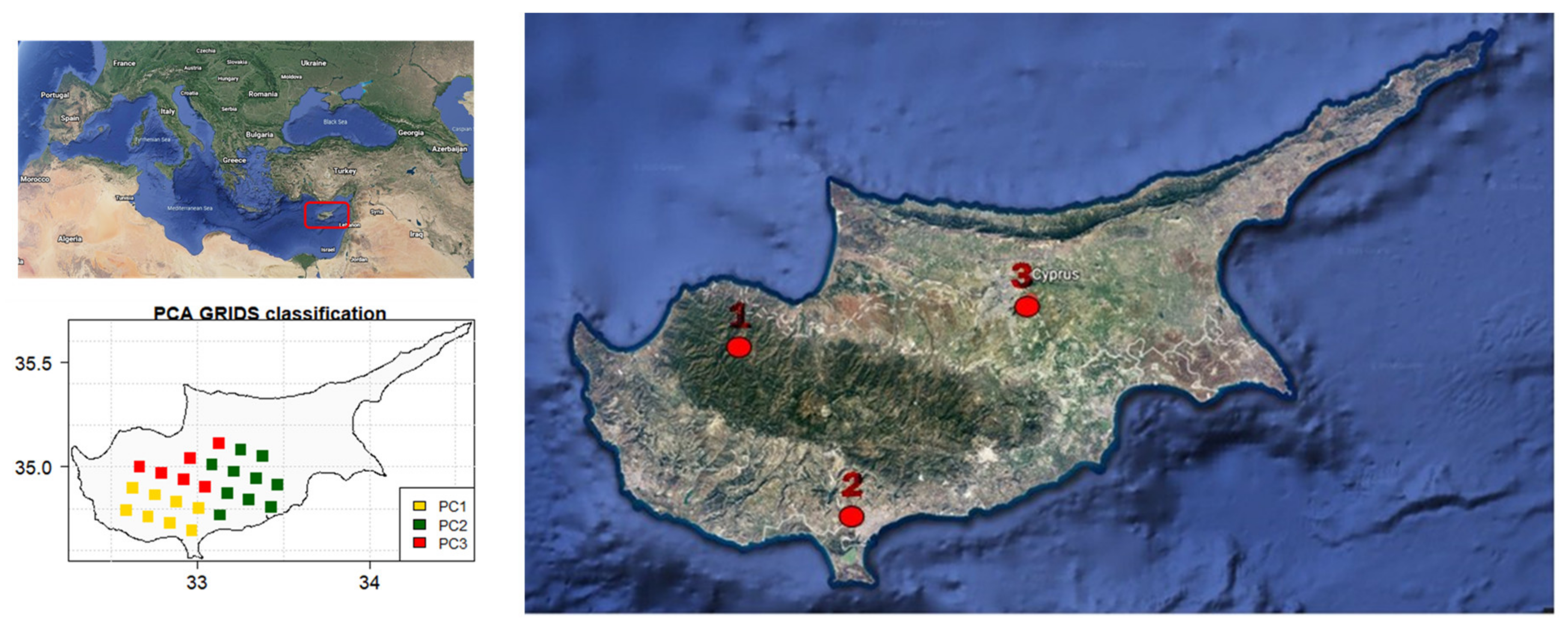
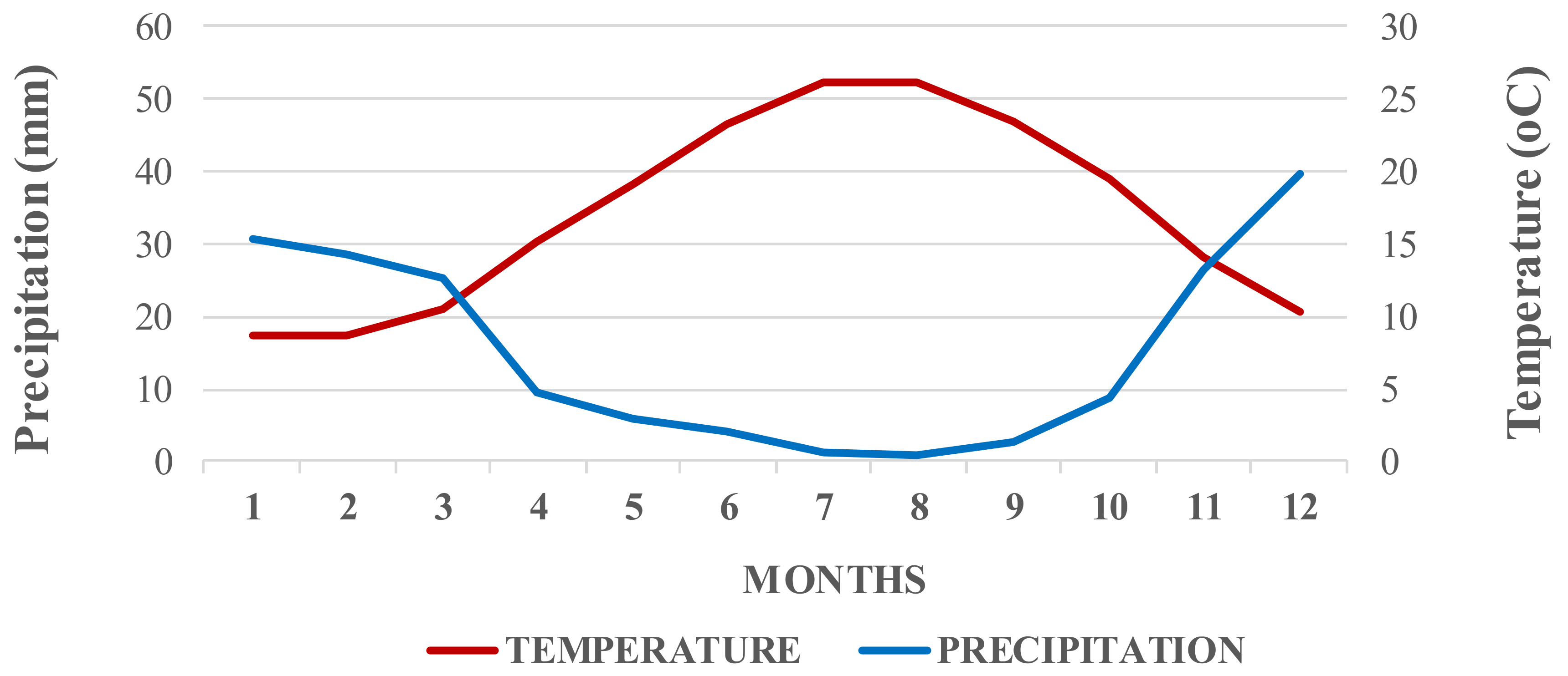
2.1. Study Area and Climate Characteristics

Cyprus is the third largest island in Mediterranean (after Sicily and Sardinia), located in the Eastern part (Figure 1). It consists of regions with different topographical and climatological characteristics, making the island an interesting area for study. Olympus (1951 m) is the highest peak of the Troodos mountain chain, which covers the central-west part of the island. Thus, the greatest precipitation amounts during all seasons are recorded there [34]. Specifically, the mean annual precipitation amount in Cyprus is around 500 mm while in Troodos peaks this amount reaches the 1100 mm. In general, Cyprus experiences a temperate climate, with warm and dry summers and mild, moderately wet winters [35]. This is also illustrated on the Bagnouls–Gaussen’s ombrothermic diagram [36] of this area (Figure 2), estimated for the period 1986–2000, using data from 10 stations that approximately uniformly cover the study area. The wettest months are November to March, while from June to September the precipitation amounts are almost zero. This results in the characterization of Cyprus as a water-stressed island [37], which underscores the need for accurate precipitation estimations.

2.2. Data

The present study uses daily precipitation data from 34 meteorological stations (Table 1, Figure 3—red and yellow points), located in the central and southwestern region of Cyprus. Station observations were provided by the Cyprus Department of Meteorology and include only those within the area controlled by the Republic of Cyprus. This dataset covers the period from 1986 to 2000 (15 years). Ten of the 34 stations were used for the formation of the TIN network and for the development of the TIN-Copula’s mathematical structure (default stations) (Table 1: stations with *, Figure 3—red points) while the other 24 stations were used for the evaluation of the results (Table 1, Figure 3—yellow points). The selection of the 10 stations was made in order to formulate a TIN network that leaves as many stations as possible for evaluation, and at the same time to cover the studied area uniformly.
Besides the station data, we analyze daily precipitation values from the CNRM-ALADIN63 Regional Climate Model [38] (Figure 3—blue points). It encompasses the broader European region, including Cyprus, with a horizontal resolution of 12.5 × 12.5 km. We have selected the model data for three different time periods: a historical one (1986–2000) and two future periods (2051–2065 and 2086–2100). The model data were produced under the European initiative of the Coordinated Regional Downscaling Experiment (EURO-CORDEX [39], domain EUR-11), and the initial and boundary conditions came from the CNRM-CM5 global climate model. For the period of 1986–2000 the model uses historical data, while for the future periods the “high emissions” (business-as-usual) pathway RCP8.5 is used [40]. The selection of the CNRM-ALADIN63 EURO-CORDEX model was motivated by the strong positive biases between the simulated and observed precipitation in Cyprus. Consequently, the recently introduced TIN-Copula method was tested for its ability to minimize these strong biases.

2.3. Methodology

The recently introduced statistical method, the TIN-Copula” method [32], is used for the bias correction of total and extreme precipitation values of the “CNRM-ALADIN63” climate simulation. The TIN-Copula method is a combination of the triangular irregular networks (TIN) and Copulas. The triangular irregular networks are a widely used tool for the representation of continuous surfaces with non-overlapping triangles [41]. The triangle formation is performed according to the Delaunay triangulation [42], using the available irregular points (e.g., stations longitude–latitude). The second component of the TIN-Copula method, copulas, are used for modeling the dependence of two or more variables [43]. This is achieved with the estimation of a new function (copula-family), which is the joint distribution of the studied variables. The main advantage of copulas is their ability to compute the dependence between variables with different marginal distributions and to examine it not only linearly but rather its whole structure [44].
For the application of the TIN-Copula method, the further 8 steps are followed:
(1)
The monthly total and extreme precipitation values were estimated from the daily data series (observed and model). As a metric for extreme precipitation, the 99th percentile of the daily precipitation values for each month was selected, based on the literature [45]. Consequently, using the initial daily data series, the monthly data series were calculated for the two studied variables (total and extreme precipitation).
(2)
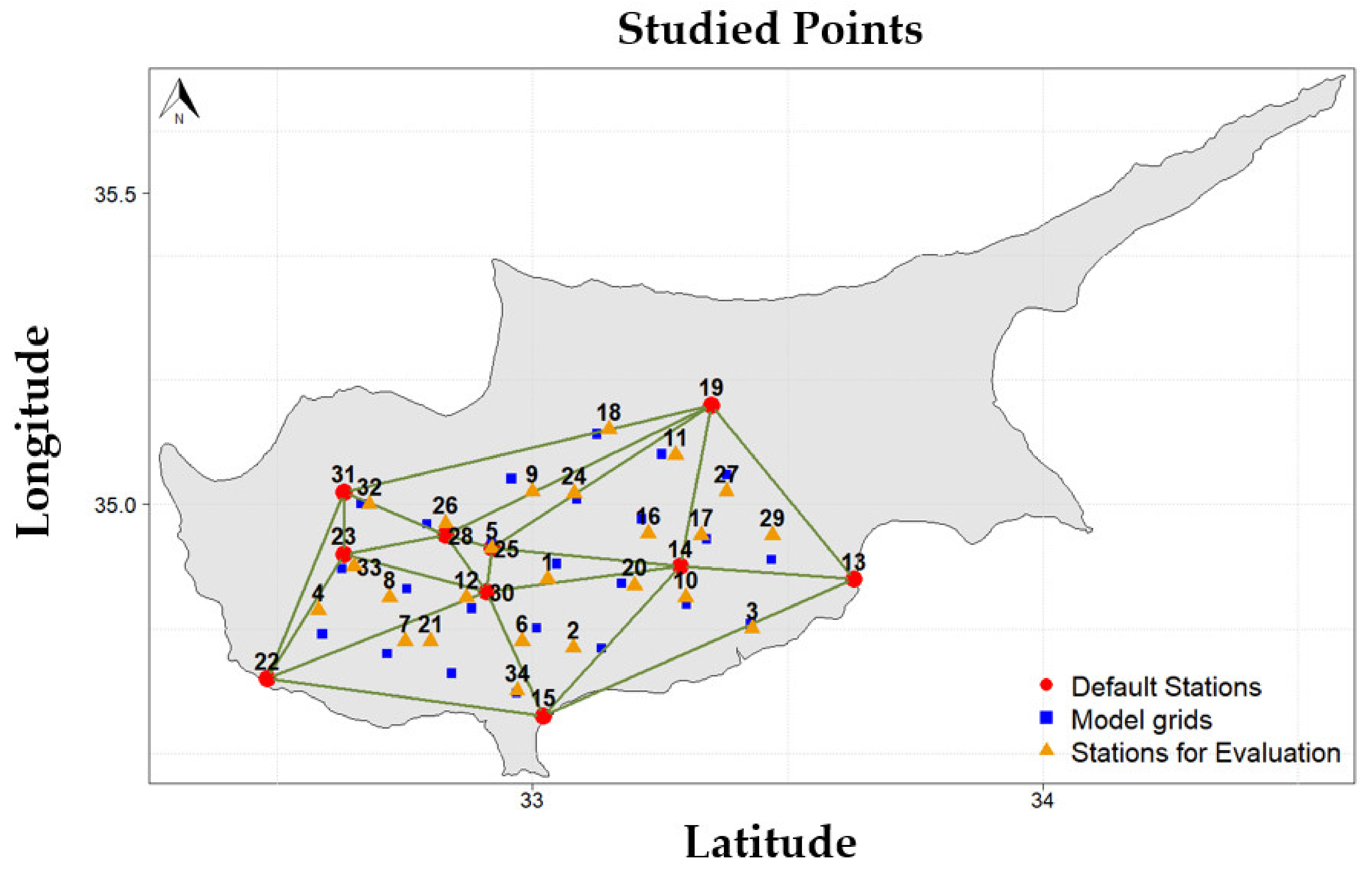
Bias correction with the TIN-Copula method starts with the TINs formation. Ten stations (Table 1: stations with *, Figure 3: red points) are selected attending the Cyprus area to be covered by triangles (Figure 3: green triangles). The TIN network formation was based on the Delaunay triangulation [42] and, as a consequence, the formatted triangles are non-overlapping. Bias correction with the TIN-Copula method can be applied to every model grid point within these triangles.
(3)
Two main calculations are carried out at the triangles’ vertices (10 default stations), using only the observed data. More specifically:
(a)
At every vertex (station) of the formatted triangles, more than 20 copula families (including the rotated versions) (Table 2) are tested in order to select the most appropriate one for the description of the studied variables dependence. The selection of the final copula family is made according to the AIC [46] and BIC [47] criteria. The robustness of the selection is higher when the length of the data series is greater.
(b)
Apart from the copula family selection, the mathematical distributions (marginals) that satisfactorily fit the studied variables are also selected. Six commonly used distributions are tested (normal, log-normal, Gamma, Pareto, generalized extreme value distribution (GEV), Weibull) and the final selection relies on the same criteria (AIC, BIC).
(4)
The second round of the estimations is focused on the model grid points—the x-points (Figure 3—blue points).
(a)
Initially, the distances between each x-point (model grids) and the vertices within the triangle are calculated (Figure 3: red points), resulting in a distance index (Wn, n = 1...3 n: the triangle vertices). The greatest value of the distance index is calculated for the vertex with the largest distance.
(5)
Combining the distance index (W) with the selected copula families of the respect vertices (n), a new function—a new copula family—was calculated at every x-point. Thus, the influence of every vertex copula family on the final new copula is inversely proportional to the respective distance.
(6)
A similar procedure (combination of distance index with the selected functions) is followed for the combination of the studied variables marginal distributions at the x-point.
(7)
Consequently, for every studied point (x-point) a unique function—a unique new copula family—is calculated. Similar calculations for the new marginal function at the x-point are followed.
(8)
The final step of the bias-correction procedure is the use of the x-point values (model values) as inputs in the corresponding new copula function. The output of this function is a normalized dataset, which is fitted by the estimated marginal function. The result is the final bias-corrected dataset.
The evaluation of the method and the analysis of the results were made separately for the historical and future periods. For the historical period, the model values (before and after bias correction) were compared with the nearest station (Figure 3—yellow points) —stations for evaluation. Additionally, the statistical significance of these biases was estimated using the t-test with a critical value of 0.05. For the future periods, the TIN-Copula network functions from the historical period (1986–2000) and from the 10 default stations are used for the bias correction of the model projections at the points that are included in the TIN. The initial model projections are compared with the corresponding bias-corrected data, while an additional analysis of the climate change signal (CCS) is performed.
The data management and analysis were performed using R programming language [48] and mainly the packages: “spcopula” [49], “copula” [50] and “VineCopula” [51].

3. Results

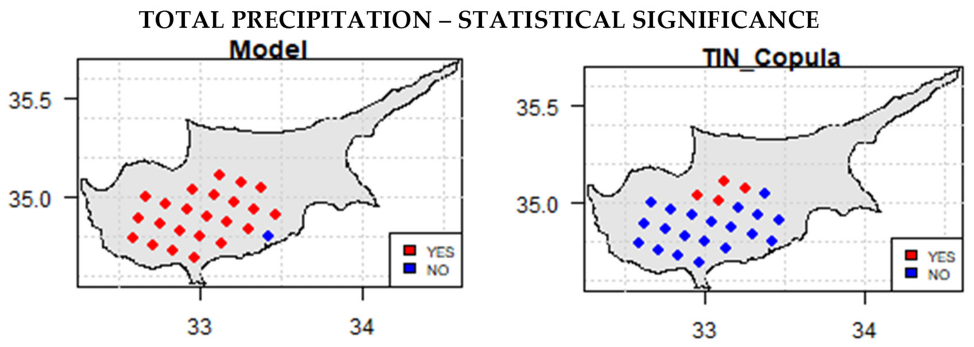
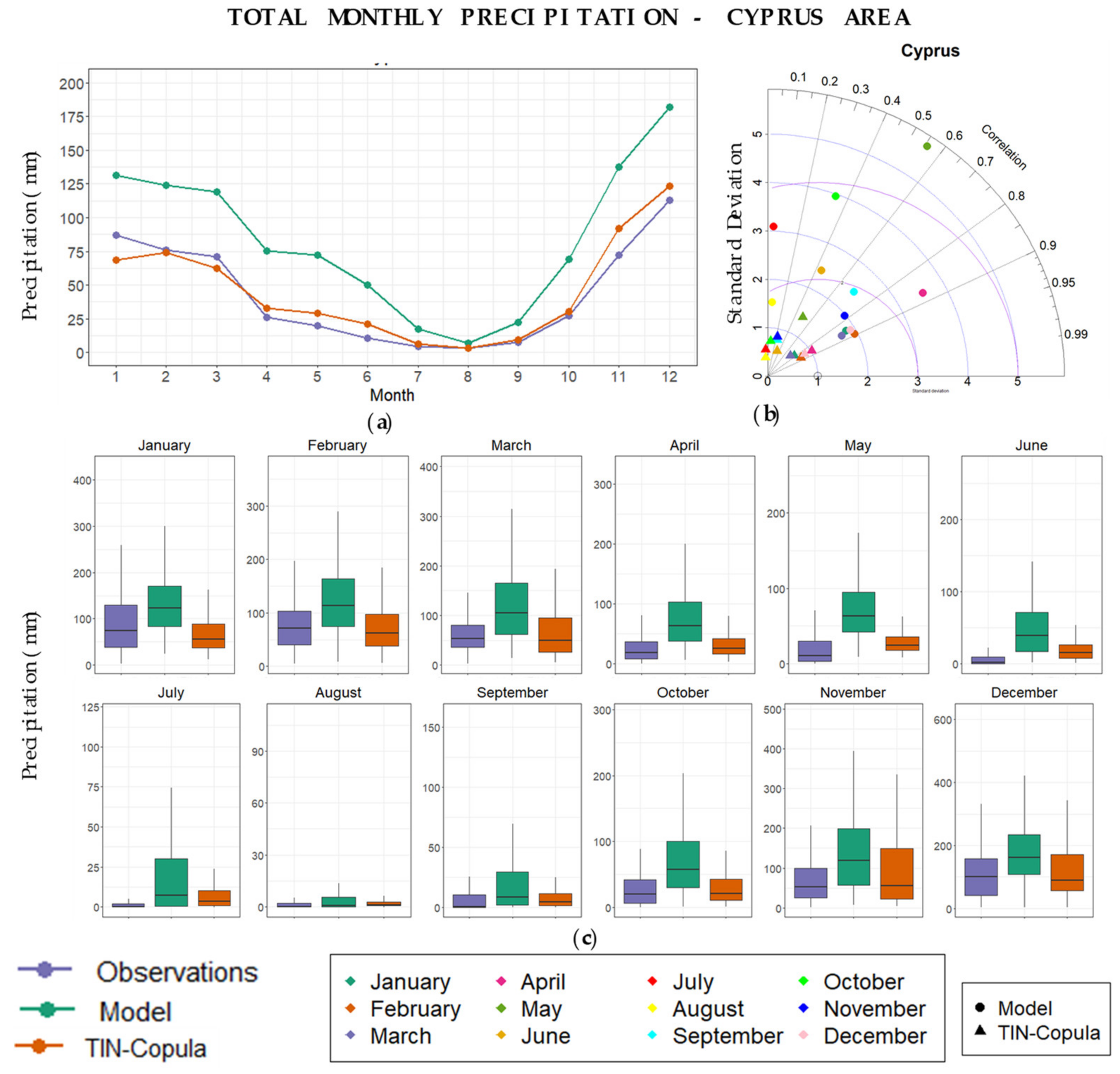
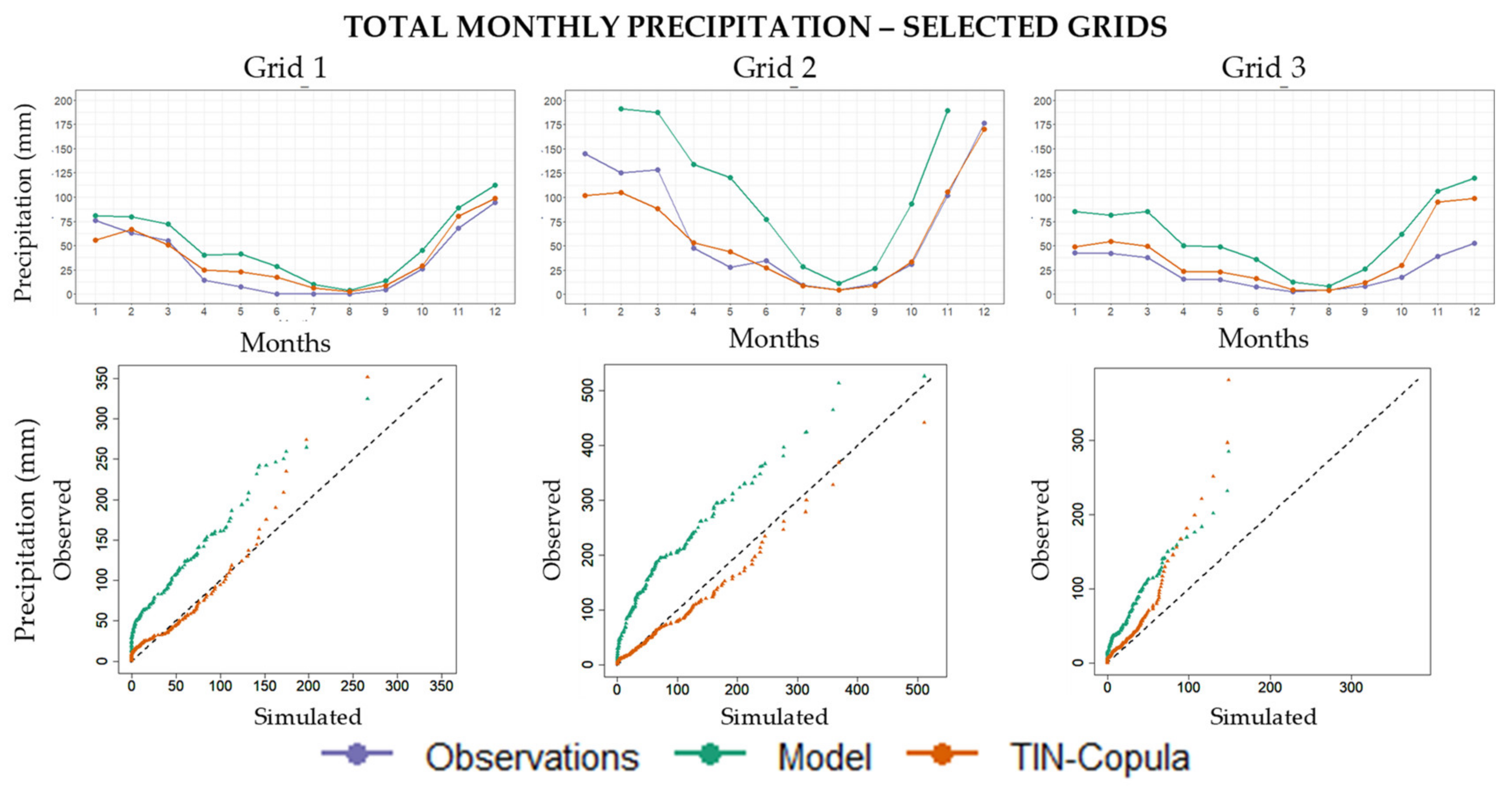
3.1. Historical Period (1986–2000)

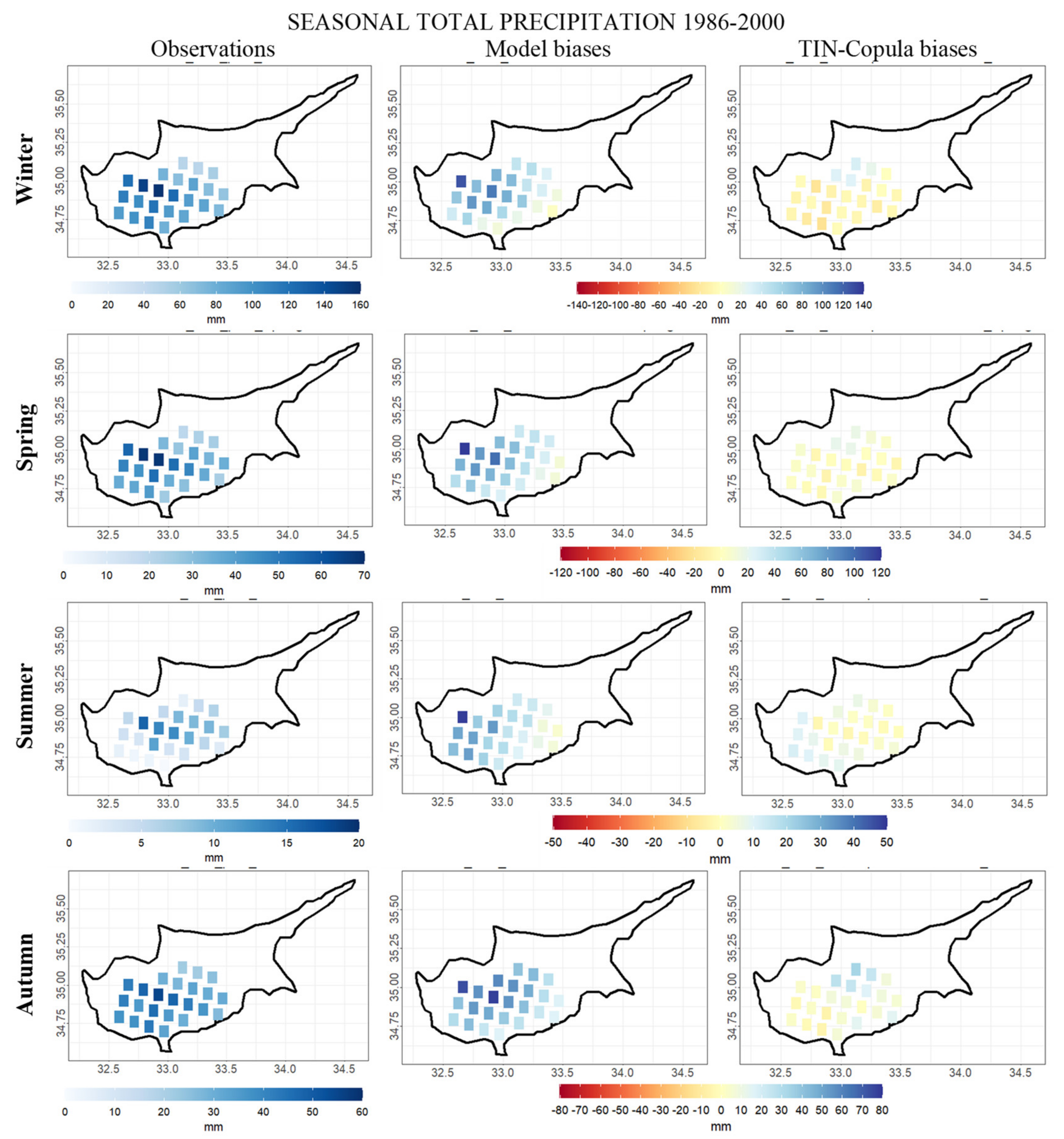
3.1.1. Seasonal and Annual Total Precipitation

Figure 4 presents the observed seasonal total precipitation values for the period of 1986–2000 (left panels), as well as the biases between these values and the model simulations, before and after bias correction (right panels). The figure reveals that the climate model substantially overestimates the observed totals in the mountainous grid cells during all seasons, while the biases are smaller in the southern and western part of the study area. The observed biases are strongly reduced after applying the TIN-Copula method. The improvement is achieved for the majority of grids and during all seasons. A representative example is apparent for the mountainous grids (Troodos chain) of the winter maps, where the biases between observations and the model’s estimations are reduced from approximately 100 to 10 mm.
An annual overview of the improvement after bias correction is depicted in Figure 5. This figure presents the locations, that is, the grids where the recorded biases are statistically significant (red points), before and after bias correction. As a limit of significance, the 95% confidence level was selected. It can be seen that the initial model values differ significantly from the observed ones in almost all grids, while after using the TIN-Copula method, the biases remain statistically significant only in a small area in the north.
Figure 6 presents the monthly mean values of total precipitation in Cyprus with line plots (Figure 6a), Τaylor diagrams (Figure 6b) and box-whisker plots (Figure 6c). According to Figure 6a,c, the model simulates total precipitation amounts, which are found to substantially exceed the observed values during all months. The overestimation is systematically higher than 50mm in several months (January to May and November to December) (Figure 6a). These findings demonstrate the need for applying a bias-correction method. The TIN-Copula method appears to be an adequate choice, which is apparent in Figure 6a,c. After bias correction, the model results closely resemble the observed values with high accuracy, as the biases are smaller than 20 mm. The minimum differences are observed on February and from July to October, while the greatest occur in January. Interestingly, the bias-corrected sample tends to somehow underestimate the observed totals, in contrast to the initial values.
The observed changes after bias correction are also illustrated in a Τaylor diagram (Figure 6b). Specifically, both the standard deviation (SD) and root mean square error (RMSE) between the observations and the model simulations are reduced after bias correction, while the correlations tend to remain similarly high during most months (exceptions: September, November, June).
For a further understanding of the TIN-Copula method efficiency, the results from three selected grid points (Figure 1) are presented in Figure 7. For the selection of the three points, a principal component analysis (PCA) was applied to precipitation values. According to the PCA results, the study area was classified into three sub-areas (Figure 1—bottom left map). One point was selected from each sub-region for an extra analysis. The first point (Grid 1) represents a coastal area, the second (Grid 2) a mountainous area and the third (Grid 3) a continental part of the island.
The model overestimates the observations in all grids, regardless of topographical characteristics (Figure 7). The main overestimation is found in the mountainous grid (Grid 2), where the largest rainfall totals occur. On the other hand, only minor biases are found for the coastal grid (Grid 1), despite the fact that in the continental grid (Grid 3) the recorded total amounts were lower. As expected from the results presented above, the main biases occur during the months with the largest totals while the smallest occur during summer when the amounts are almost zero. However, slight overestimations are found in the summer months, leading to an overestimation that can exceed 100% (e.g., September, Grid 2).
The calculated biases between the initial model results and the observations are additionally illustrated in quantile–quantile plots (QQ plots), in which the model values diverge importantly from the diagonal 1:1 line (Figure 7—bottom panels). The application of the TIN-Copula method improves the initial values in all grids and during almost all months. The greatest reduction in the biases is achieved on the mountainous grid (Grid 2), where the TIN-Copula values approach the observations with high accuracy, especially during the period from April to December. This is also confirmed by the respective QQ plot, as the TIN-Copula bias-corrected values are very close to the reference line. The effectiveness of the TIN-Copula method is also obvious on the other two grids (Grid 1 and 3), despite the fact that the initial biases are lower than the mountainous grid. For instance, for the continental grid (Grid 3), the model simulates higher totals than the observed ones during the whole year. The TIN-Copula method significantly reduces these differences, especially in the first 10 months of the year.

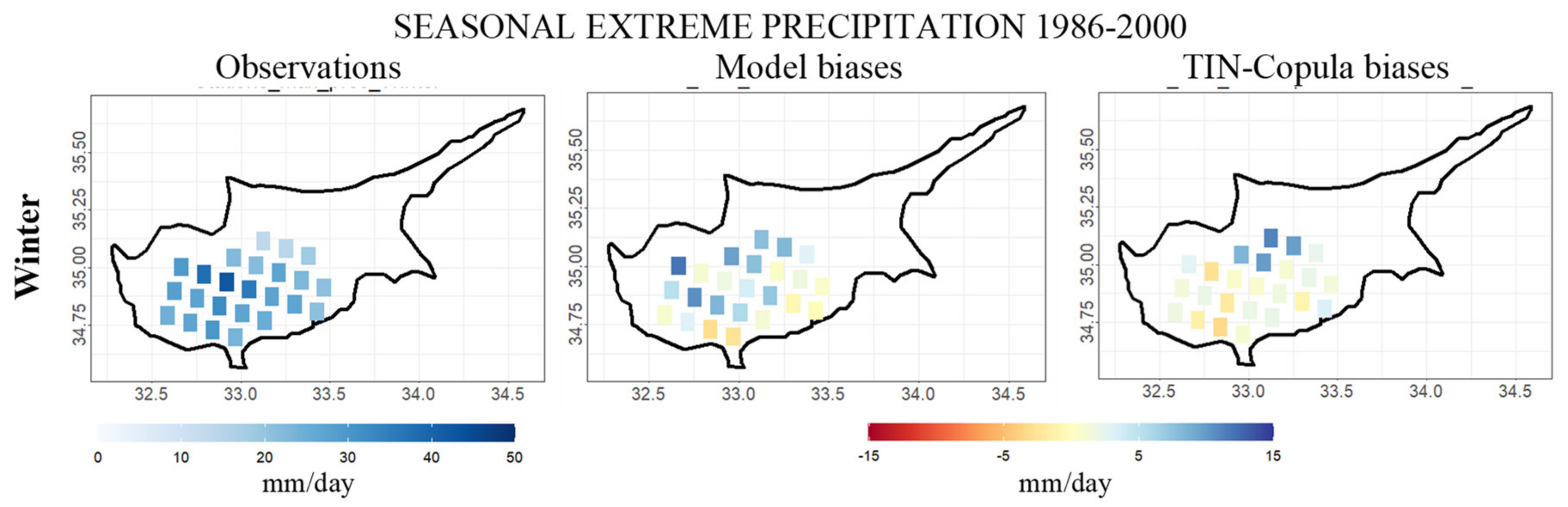
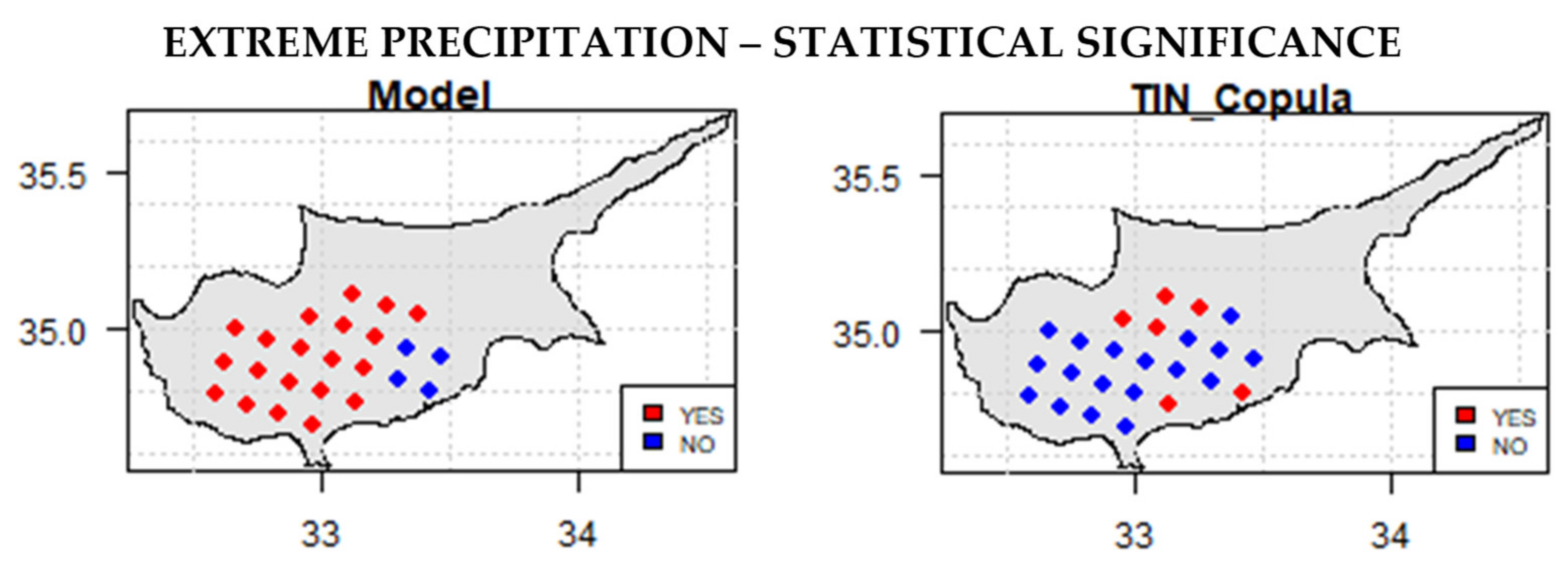
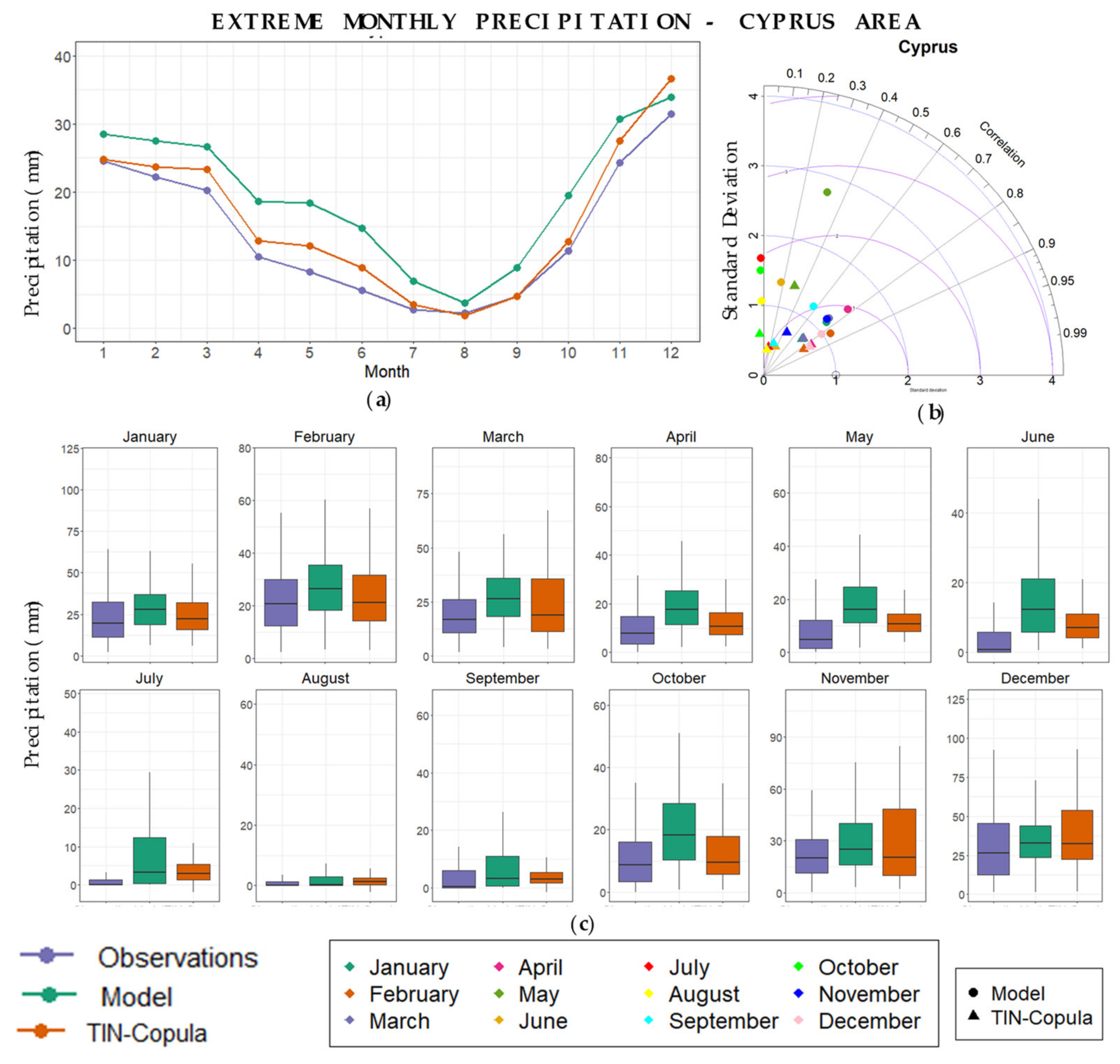
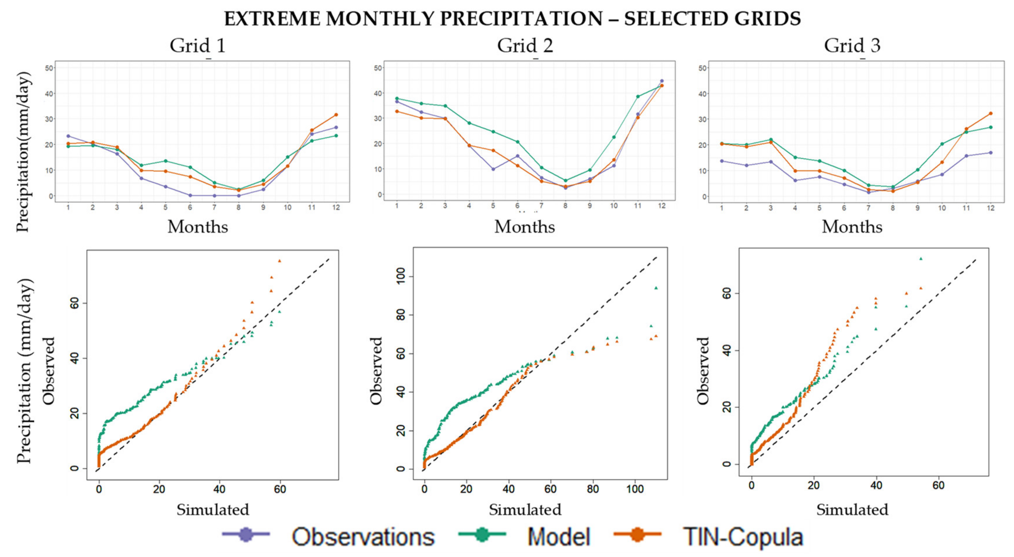
3.1.2. Seasonal and Annual Extreme Precipitation
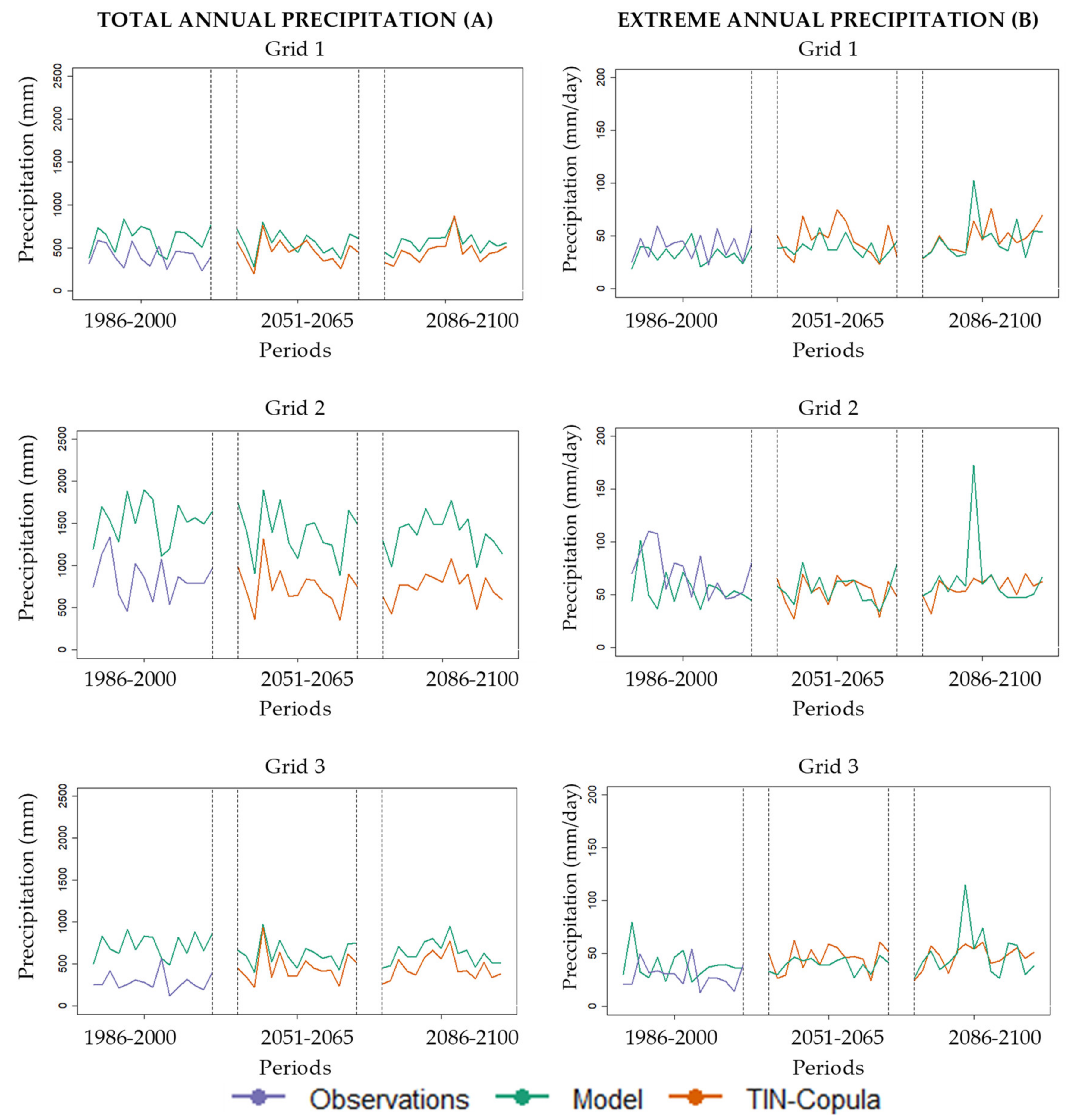
Figure 8 presents the observed extreme precipitation rates during winter (>99%) (left panel) as well as the biases between these values and the model simulations (before and after bias correction, right panels). During winter, when the extremes are most common, the results for the western and southeastern coastal grids are satisfactory, while in the remaining area some model overestimate by 5 to 15 mm/day. The TIN-Copula method thus improves the results in the largest part of the study area, however, a larger overestimation (than that of the uncorrected RCM) is evident for the northeastern grid cells. This pattern presents some similarities with autumn (not shown) when the extremes are well simulated on the western and northern coastal areas. For the remaining seasons (not shown), the highest biases occur in the western and mountainous grid points, while the lowest are in the southeast part. The common result for all seasons is that the TIN-Copula method minimizes the differences in the majority of grids and especially those with the largest biases. Additionally, the effectiveness of the TIN-Copula method is not shown to be relevant for the reduction in absolute biases (Figure 8, maps of the other seasons—not shown) but also changes the biases from being statistically significant to non-significant (Figure 9).
The monthly analysis of extreme precipitation rates in Cyprus (Figure 10) reveals that the model clearly overestimates the observed extremes during the whole year (Figure 10a,c). The largest overestimations occur in April, May and June (~10 mm) and the smallest in August, when the mean value of stations extremes is 4 mm. For the other months, the biases range from 4 to 7 mm/day (Figure 10a), calculated from the ensemble (Figure 10c) and not only from the stations with the greatest values. The use of the TIN-Copula method improves the results for almost all months (except for December) as the remaining biases range from zero (January and July–October) to five mm/day (May). The SD and the RMSE values corroborate this improvement, as they have also been reduced by the bias correction. Finally, a slight increase in the correlation values is achieved for several months (Figure 10c).
A further analysis of extreme precipitation for three selected grid points with different topographical characteristics (Figure 1) is presented in Figure 11. The results show that in all grid points, the model tends to simulate more intense extremes compared with the observed ones, while the TIN-Copula’s values are much closer. This is also obvious in the QQ plots in which the non-corrected values diverge importantly from the diagonal line, while the corrected ones approach it with high accuracy. The largest correction is achieved for the mountainous grid (Grid 2) where the biases were almost eliminated in nine of the 12 months after applying the TIN-Copula method. A similar significant improvement is also achieved during the winter and autumn months in the coastal grid (Grid 1) and during the summer months in the continental grid (Grid 2). In general, after bias correction, the observed extremes are estimated with higher accuracy in most of the other months. An increase in the biases is identified in December for both the coastal and the continental grids, while during the other two winter months (January, February), the biases remain the same before and after bias correction.

3.2. Future Periods

Projections

The second objective of this study is to analyze the climate model projections for total and extreme precipitation before and after the use of the TIN-Copula method. Figure 12 provides an annual overview of the model results (initial and bias-corrected) for the two selected future periods (2051–2065 and 2086–2100), as well as the observed and simulated values during the historical period (1986–2000). The results are presented for the three selected grid points (Figure 1) which have different topographical and consequently climatological characteristics.
Figure 12A (left panels) reveal that the model tends to project higher totals before the use of the TIN-Copula copula method, in all grid points and for both future periods. This difference is larger in the mountainous grid (Grid 2) where the model also significantly overestimates the observed values during the historical period. In the other two grids the differences are smaller, as well as those during the historical period.
The projected extreme annual precipitation (Figure 12B—right panels) shows different performance compared to the annual totals (Figure 12A). The projected values before and after bias correction tend to be close in all grids and for both future periods. However, greater differences occur in specific years, mainly in the second future time period (2086–2100).

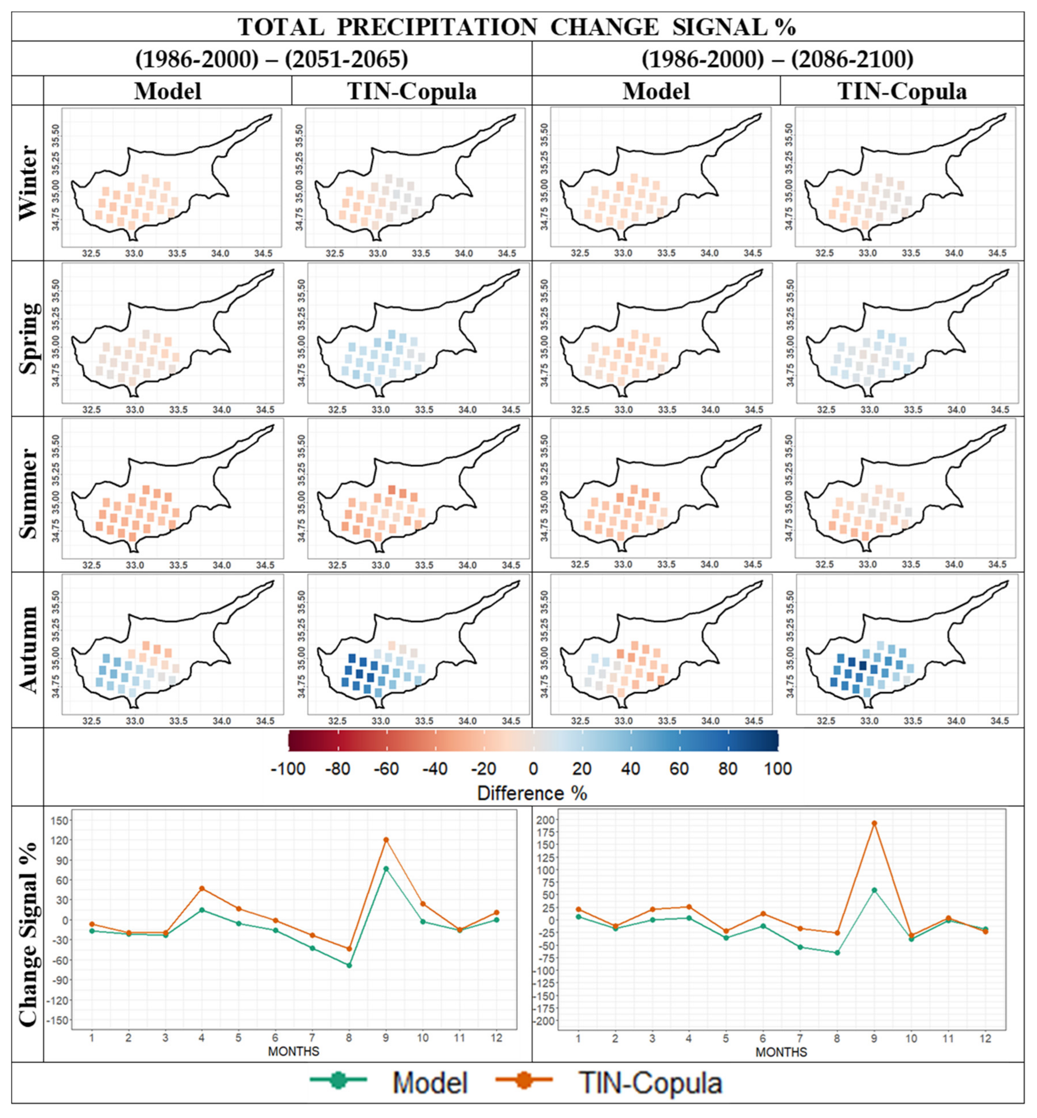
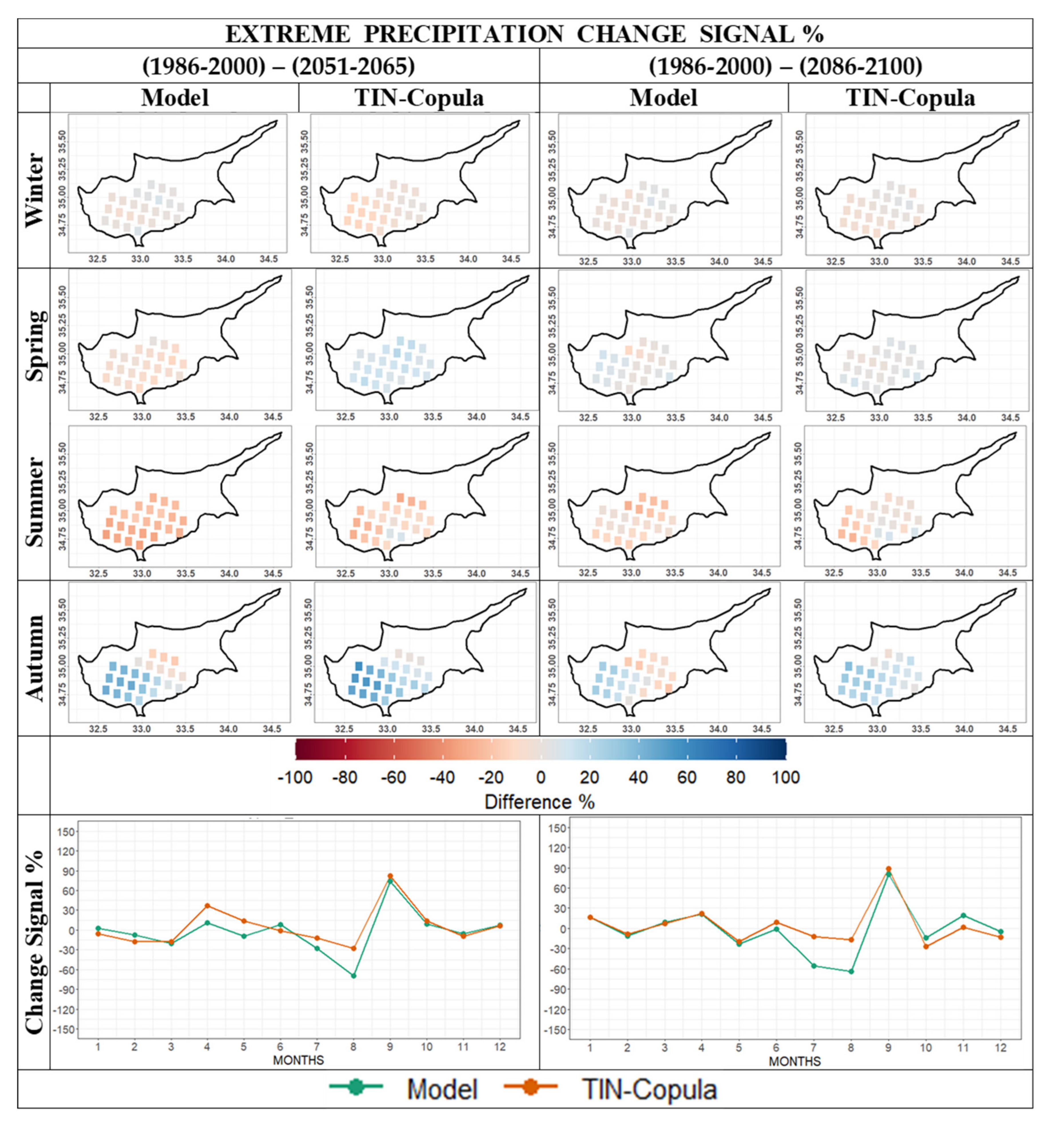
3.3. Climate Change Signal

We additionally investigated the possible impact of a bias-correction method on the precipitation climate change signal (CCS) for two future periods (Figure 13). In winter, the TIN-Copula method does not affect the CCS in the western part of the studied area, while on the eastern part an increase of around 10% is apparent in both future periods. Different results appear for spring, showing that the use of the bias-correction method changes the signal values from negative to positive. This result is also illustrated in the annual cycle plots of the corresponding periods, in which the mean area values of the CCS are around zero (March, April, May), but sometimes they exceed this limit and sometimes they are below. For the summer season, the negative CCS remains almost constant after the use of the TIN-Copula method for the first future period (2051–2065), while for the second one (2086–2100) an increase is found in the eastern part. The season during which the bias-correction method mostly affects the CCS values is autumn. Both the maps and the corresponding annual cycles indicate that changes mainly occur during September, especially in the second time period. During mid-century, 2051–2065, the CCSs before bias correction are within 20% in most of the study area, while in the eastern grids they are negative (–20%). This pattern remains after bias correction, but the values are greater at all locations. During the second time period, the CCSs before bias correction are negative in the majority of grids (exception: the northwest area), whereas after the use of the TIN-Copula method, the signals exceed 40% in most grid points. This is also illustrated by the monthly line plots (Figure 13), which reveals that this change happens only during September, while in October and November the mean CCS does not change.
Figure 14 presents the CCS of extreme precipitation before and after bias correction. The result for the winter show that the TIN-Copula method does not significantly affect the CCS, both during 2051–2065 and 2086–2100. This is corroborated by the line plots, as the differences between the two studied samples are almost zero (January, February, December). This is also evident during spring but only for the second time period (2086–2100). In the first one, the bias-corrected sample tends to estimate a higher CCS, changing the signal from generally negative to positive. The monthly analysis shows that there is not a CCS reversal in the spring months individually but only in the mean seasonal value. The summer is a period when lowest number of precipitation extremes occur. The CCS changes are below a maximum of 5 mm/day. The summer results reveal that after bias correction the CCSs are higher than initially in the whole area for both study periods. The increase in the CCS is larger in the western grids and for the second time period. The corresponding line plots (Figure 14—bottom panels) provide some additional information, indicating that the suggested differences mainly occur due to the CCS in August in the first period and in July and August during the second. During autumn, the model seems to project an increase in extremes in the western part of the area and a decrease in the eastern part. The same pattern also after the TIN-Copula correction, but the CCSs are larger than initially. However, the mean CCSs over the whole area and autumn show no change. Finally, in the last 15 years of the 21st century, the model continues projecting an increase in the western part and a decrease in the eastern part of the domain. However, after bias correction, the CCSs are larger than they initially were, and the inverse is found for the eastern grid points.

4. Discussion and Conclusions

The present study used a recently developed statistical method—the TIN-Copula method—for the bias correction of total end extreme precipitation values, simulated by the CNRM-ALADIN63 regional climate model for the region of Cyprus. The bias-correction procedure was applied to one historical (1986–2000) and two future periods (2051–2065 and 2086–2100). This research is the first attempt to thoroughly examine the ability of the TIN-Copula method to improve the regional climate model output for a future period, as well as for the parameter of total precipitation.
Our results show that the climate model tends to overestimate the observed total and extreme precipitation in much of the studied area for the whole time period considered. The discrepancies can be partly explained by the inability of the climate models to project total and extreme precipitation over complex topography in the Mediterranean area—especially in the eastern part, which is predominantly upwind of weather systems that are associated with precipitation [52,53]. Tramblay et al. [54] who used the same climate model for another south Mediterranean region, Morocco, emphasized the need for bias correction. The TIN-Copula method seems to be a useful tool for the improvement of total and extreme precipitation, as the bias-corrected values approach the observed ones with high accuracy. The improvement in modelled extremes (temperature and precipitation percentiles) was previously achieved for several Mediterranean stations for the period of 1981–2000 [33]. The main improvement is achieved for mountainous areas, where the climate model also has largest biases. This is in accord with Zittis et al. [37] who mentioned that the large biases in mountainous grids are related to the 12-km resolution, which does not adequately represent steep orographic gradients. An advantage of the TIN-Copula method is that is only uses observed data for the formation of a unique TIN-Copula model for each region, resulting in significant reductions in the biases.
The study results for the two future periods reveal that the bias-corrected total and extreme precipitations are lower than the initial model projections. This mainly refers to the winter months with relatively high precipitation amounts, rather than the summer season when it is mostly dry [55], for which the projections are very similar before and after bias correction. Furthermore, comparable to the historical results, the largest differences for the projections occur in the grids at highest elevation. These results are in accord with Giannakopoulos et al. [56], who analyzed a six-model ensemble for Cyprus, projecting a general decrease in the annual total precipitation, especially in the Troodos Mountains.
The reduction in the projected model precipitation after bias correction is illustrated in the climate change signal (CCS). The bias-correction effects on the CCS depends on several factors, such as the selected model, method, parameter or the studied area [57]. In this study, the CCS in total and extreme precipitation tends to increase by bias correction, for both parameters and projection periods. The mean monthly CCSs for the entire area are nearly unchanged for the wettest months and those with the strongest extremes. The main differences between the initial and the bias-corrected CCSs occurred in the months with lowest precipitation amounts (an increase from 0mm to 1mm is counted as 100%). Similar results are reported by Eum et al. [58], who argue that the relationship between a bias-correction method and the CCS is considerably negative for model simulated precipitation. Furthermore, some changes depend on the selected historical period. The historical period for which the CCS has been derived, as well as the assumption that the biases are the time-invariant, are important factors to be considered [16].
In conclusion, our results show that the TIN-Copula method is a useful tool for bias correction. Since it was recently introduced, further research should be undertaken to investigate the efficiency of the method for larger areas and other parameters, as well as for different regional and global climate model results.

Author Contributions

Conceptualization, G.L., G.Z. and C.A.; Data curation, G.L. and G.Z.; Investigation, G.L.; Methodology, G.L., G.Z. and C.A.; Software, G.L. and C.A.; Supervision, G.Z., C.A., P.H. and J.L.; Visualization, G.L.; Writing—original draft, G.L.; Writing—review & editing, G.Z., C.A., P.H. and J.L. All authors have read and agreed to the published version of the manuscript.

Funding

This research was funded by the EMME-CARE project that has received funding from the European Union’s Horizon 2020 Research and Innovation Programme, under grant agreement no. 856612, as well as matching co-funding by the Government of the Republic of Cyprus.

Acknowledgments

We acknowledge the Department of Meteorology of the Republic of Cyprus for providing the station observations and the data providers of the EURO-CORDEX ALADIN63 experiments.

Conflicts of Interest

The authors declare no conflict of interest.

References

  1. Intergovernmental Panel on Climate Change. Climate Change 2013—The Physical Science Basis: Working Group I Contribution to the Fifth Assessment Report of the Intergovernmental Panel on Climate Change; Cambridge University Press: Cambridge, UK; New York, NY, USA, 2013. [Google Scholar] [CrossRef] [Green Version]
  2. Flato, G.; Marotzke, J.; Abiodun, B.; Braconnot, P.; Chou, S.C.; Collins, W.; Cox, P.; Driouech, F.; Emori, S.; Eyring, V.; et al. Evaluation of climate models. In Climate Change 2013: The Physical Science Basis. Contribution of Working Group I to the Fifth Assessment Report of the Intergovernmental Panel on Climate Change; Cambridge University Press: Cambridge, UK; New York, NY, USA, 2014; pp. 741–866. [Google Scholar]
  3. Giorgi, F.; Gary, T.B. The climatological skill of a regional model over complex terrain. Mon. Weather Rev. 1989, 117, 2325–2347. [Google Scholar] [CrossRef] [Green Version]
  4. Goody, R.; Anderson, J.; North, G. Testing climate models: An approach. Bull. Am. Meteorol. Soc. 1998, 79, 2541–2549. [Google Scholar] [CrossRef] [Green Version]
  5. Suklitsch, M.; Gobiet, A.; Truhetz, H.; Awan, N.K.; Göttel, H.; Jacob, D. Error characteristics of high resolution regional climate models over the Alpine area. Clim. Dyn. 2011, 37, 377–390. [Google Scholar] [CrossRef] [Green Version]
  6. Kumar, D.; Kodra, E.; Ganguly, A.R. Regional and seasonal intercomparison of CMIP3 and CMIP5 climate model ensembles for temperature and precipitation. Clim. Dyn. 2014, 43, 2491–2518. [Google Scholar] [CrossRef]
  7. Mearns, L.O.; Arritt, R.; Biner, S.; Bukovsky, M.S.; McGinnis, S.; Sain, S.; Caya, D.; Correia, J., Jr.; Flory, D.; Gutowski, W.; et al. The North American Regional Climate Change Assessment Program: Overview of phase I results. Bull. Am. Meteorol. Soc. 2012, 93, 1337–1362. [Google Scholar] [CrossRef]
  8. Sillmann, J.; Kharin, V.V.; Zhang, X.; Zwiers, F.W.; Bronaugh, D. Climate extremes indices in the CMIP5 multimodel ensemble: Part 1. Model evaluation in the present climate. J. Geophys. Res. Atmos. 2013, 118, 1716–1733. [Google Scholar] [CrossRef]
  9. Lung, T.; Dosio, A.; Becker, W.; Lavalle, C.; Bouwer, L.M. Assessing the influence of climate model uncertainty on EU-wide climate change impact indicators. Clim. Chang. 2013, 120, 211–227. [Google Scholar] [CrossRef]
  10. Ban, N.; Schmidli, J.; Sch¨ar, C. Heavy precipitation in a changing climate: Does short-term summer precipitation increase faster? Geophys. Res. Lett. 2015, 42, 1165–1172. [Google Scholar] [CrossRef]
  11. Torma, C.; Giorgi, F.; Coppola, E. Added value of regional climate modeling over areas characterized by complex terrain-precipitation over the Alps. J. Geophys. Res. Atmos. 2015, 120, 3957–3972. [Google Scholar] [CrossRef]
  12. Mitchell, T.D.; Hulme, M. Predicting regional climate change: Living with uncertainty. Prog. Phys. Geog. 1999, 23, 57–78. [Google Scholar] [CrossRef]
  13. Hall, A. Projecting regional change. Science 2014, 346, 1461–1462. [Google Scholar] [CrossRef] [PubMed]
  14. Ramirez-Villegas, J.; Challinor, A.J.; Thornton, P.K.; Jarvis, A. Implications of regional improvement in global climate models for agricultural impact research. Environ. Res. Lett. 2013, 8, 024018. [Google Scholar] [CrossRef]
  15. Maraun, D.; Wetterhall, F.; Ireson, A.M.; Chandler, R.E.; Kendon, E.J.; Widmann, M.; Brienen, S.; Rust, H.W.; Sauter, T.; Themeßl, M.; et al. Precipitation downscaling under climate change: Recent developments to bridge the gap between dynamical models and the end user. Rev. Geophys. 2010, 48. [Google Scholar] [CrossRef]
  16. Maraun, D. Bias correcting climate change simulations-a critical review. Curr. Clim. Chang. Rep. 2016, 2, 211–220. [Google Scholar] [CrossRef] [Green Version]
  17. Sperna Weiland, F.C.; van Beek, L.P.H.; Kwadijk, J.C.J.; Bierkens, M.F.P. The ability of a GCM-forced hydrological model to reproduce global discharge variability. Hydrol. Earth Syst. Sci. 2010, 14, 1595–1621. [Google Scholar] [CrossRef] [Green Version]
  18. Navarro-Racines, C.E.; Tarapues-Montenegro, J.E.; Ramírez-Villegas, J.A. Bias-correction in the CCAFS Climate. In Portal: A Description of Methodologies. Decision and Policy Analysis (DAPA) Research Area; International Center for Tropical Agriculture (CIAT): Cali, Colombia, 2015. [Google Scholar]
  19. Shrestha, M.; Acharya, S.C.; Shrestha, P.K. Bias correction of climate models for hydrological modelling–are simple methods still useful. Meteorol. Appl. 2017, 24, 531–539. [Google Scholar] [CrossRef] [Green Version]
  20. Tabor, K.; Williams, J.W. Globally downscaled climate projections for assessing the conservation impacts of climate change. Ecol. Appl. 2010, 20, 554–565. [Google Scholar] [CrossRef] [Green Version]
  21. Räty, O.; Räisänen, J.; Ylhäisi, J.S. Evaluation of delta change and bias correction methods for future daily precipitation: Intermodel cross-validation using ENSEMBLES simulations. Clim. Dyn. 2014, 42, 2287–2303. [Google Scholar] [CrossRef]
  22. Lenderink, G.; Buishand, A.; van Deursen, W. Estimates of future discharges of the river Rhine using two scenario methodologies: Direct versus delta approach. Hydrol. Earth Syst. Sci. 2007, 11, 1145–1159. [Google Scholar] [CrossRef]
  23. Willkofer, F.; Schmid, F.J.; Komischke, H.; Korck, J.; Braun, M.; Ludwig, R. The impact of bias correcting regional climate model results on hydrological indicators for Bavarian catchments. J. Hydrol. Reg. Stud. 2018, 19, 25–41. [Google Scholar] [CrossRef]
  24. Déqué, M. Frequency of precipitation and temperature extremes over France in an anthropogenic scenario: Model results and statistical correction according to observed values. Glob. Planet. Chang. 2007, 57, 16–26. [Google Scholar] [CrossRef]
  25. Ezéchiel, O.; Eric, A.A.; Josué, Z.E.; Eliézer, B.I.; Amédée, C.; Abel, A. Comparative study of seven bias correction methods applied to three Regional Climate Models in Mekrou Catchment (Benin, West Africa). Int. J. Curr. Eng. Technol. 2016, 6, 1831–1840. [Google Scholar]
  26. Maity, R. Statistical Methods in Hydrology and Hydroclimatology; Springer: Singapore, 2018; 444p. [Google Scholar] [CrossRef]
  27. Zhang, Q.; Xiao, M.; Singh, V.P.; Chen, X. Copula-based risk evaluation of hydrological droughts in the East River basin, China. Stoch. Environ. Res. Risk Assess. 2013, 27, 1397–1406. [Google Scholar] [CrossRef]
  28. Lazoglou, G.; Anagnostopoulou, C.; Skoulikaris, C.; Tolika, K. Bias correction of climate model’s precipitation using the copula method and its application in river basin simulation. Water 2019, 11, 600. [Google Scholar] [CrossRef] [Green Version]
  29. Piani, C.; Haerter, J.O. Two dimensional bias correction of temperature and precipitation copulas in climate models. Geophys. Res. Lett. 2012, 39. [Google Scholar] [CrossRef]
  30. Alidoost, F.; Stein, A.; Su, Z.; Sharifi, A. Three novel copula-based bias correction methods for daily ECMWF air temperature data. Hydrol. Earth Syst. Sci. Discuss. 2017, 1–27. [Google Scholar] [CrossRef] [Green Version]
  31. Maity, R.; Suman, M.; Laux, P.; Kunstmann, H. Bias Correction of Zero-Inflated RCM Precipitation Fields: A Copula-Based Scheme for Both Mean and Extreme Conditions. J. Hydrometeorol. 2019, 20, 595–611. [Google Scholar] [CrossRef]
  32. Lazoglou, G.; Gräler, B.; Anagnostopoulou, C. Simulation of extreme temperatures using a new method: TIN-copula. Int. J. Climatol. 2019, 39, 5201–5214. [Google Scholar] [CrossRef]
  33. Lazoglou, G.; Angnostopoulou, C.; Tolika, K.; Benedikt, G. Evaluation of a New Statistical Method—TIN-Copula–for the Bias Correction of Climate Models’ Extreme Parameters. Atmosphere 2020, 11, 243. [Google Scholar] [CrossRef] [Green Version]
  34. Camera, C.; Bruggeman, A.; Hadjinicolaou, P.; Pashiardis, S.; Lange, M.A. Evaluation of interpolation techniques for the creation of gridded daily precipitation (1× 1 km2); Cyprus, 1980–2010. J. Geophys. Res. Atmos. 2014, 119, 693–712. [Google Scholar] [CrossRef]
  35. Zittis, G.; Bruggeman, A.; Camera, C.; Hadjinicolaou, P.; Lelieveld, J. The added value of convection permitting simulations of extreme precipitation events over the eastern Mediterranean. Atmos. Res. 2017, 191, 20–33. [Google Scholar] [CrossRef]
  36. Bagnouls, F.; Gaussen, H. Saison séche et indice xérothermique. Docum. Pour Cart. Prod. Veget. Ser. Gen. 1953, 1, 1–49. [Google Scholar]
  37. Zittis, G.; Bruggeman, A.; Camera, C. 21st Century Projections of Extreme Precipitation Indicators for Cyprus. Atmosphere 2020, 11, 343. [Google Scholar] [CrossRef] [Green Version]
  38. Daniel, M.; Lemonsu, A.; Déqué, M.; Somot, S.; Alias, A.; Masson, V. Benefits of explicit urban parameterization in regional climate modeling to study climate and city interactions. Clim. Dyn. 2019, 52, 2745–2764. [Google Scholar] [CrossRef] [Green Version]
  39. Jacob, D.; Teichmann, C.; Sobolowski, S.; Katragkou, E.; Anders, I.; Belda, M.; Benestad, R.; Boberg, F.; Buonomo, E.; Cardoso, R.M.; et al. Regional climate downscaling over Europe: Perspectives from the EURO-CORDEX community. Reg. Environ. Chang. 2020, 20. [Google Scholar] [CrossRef]
  40. Riahi, K.; Krey, V.; Rao, S.; Chirkov, V.; Fischer, G.; Kolp, P.; Kindermann, G.; Nakicenovic, N.; Rafai, P. RCP 8.5-A scenario of comparatively high greenhouse gas emissions. Clim. Chang. 2011, 109, 33–57. [Google Scholar] [CrossRef] [Green Version]
  41. Peucker, T.K.; Fowler, R.J.; Little, J.J.; Mark, D.M. Digital representation of three-dimensional surfaces by triangulated irregular networks (TIN). In Technical Report #10; Programs: Contract N00014-75-C-0886; Office of Naval Research (ONR) Geography, Simon Fraser University: Burnaby, BC, Canada, 1976; 63p. [Google Scholar]
  42. Delaunay, B. Sur la sphère vide. Bull. Acad. Sci. USSR VII Class. Sci. Mat. Nat. 1934, 793–800. [Google Scholar]
  43. Nelsen, R.B. An Introduction to Copulas, 2nd ed.; Springer: New York, NY, USA, 2006. [Google Scholar]
  44. Zhang, L.; Singh, V.P. Bivariate rainfall frequency distributions using Archimedean copulas. J. Hydrol. 2007, 332, 93–109. [Google Scholar] [CrossRef]
  45. Anagnostopoulou, C.; Tolika, K. Extreme precipitation in Europe: Statistical threshold selection based on climatological criteria. Theor. Appl. Climatol. 2012, 107, 479–489. [Google Scholar] [CrossRef]
  46. Akaike, H. Information theory and an extension of the maximum likelihood principle. In Proceedings of the 2nd International Symposium on Information Theory, Tsahkadsor, Armenia, 2–8 September 1971; pp. 267–281. [Google Scholar]
  47. Schwarz, G. Estimating the dimension of a model. Ann. Stat. 1978, 6, 461–464. [Google Scholar] [CrossRef]
  48. Core Team, R. R: A Language and Environment for Statistical Computing; R Foundation for Statistical Computing: Vienna, Austria, 2018. [Google Scholar]
  49. Gräler, B. Modelling skewed spatial random fields through the spatial vine copula. Spat. Stat. 2014, 10, 87–102. [Google Scholar] [CrossRef] [Green Version]
  50. Hofert, M.; Kojadinovic, I.; Maechler, M.; Yan, J. Copula: Multivariate Dependence with Copulas, 2018, R Package Version 0.999-19. 2018. Available online: http://search.r-project.org/library/copula/html/copula-package.html (accessed on 3 July 2020).
  51. Schepsmeier, U.; Stoeber, J.; Brechmann, E.C.; Graeler, B.; Nagler, T.; Erhardt, T. VineCopula: Statistical Inference of Vine Copulas. 2018, R Package Version 2.1.8. Available online: https://cran.r-project.org/web/packages/VineCopula/VineCopula.pdf (accessed on 3 July 2020).
  52. Sevault, F.; Somot, S.; Alias, A.; Dubois, C.; Lebeaupin-Brossier, C.; Nabat, P.; Adloff, F.; Déqué, M.; Decharme, B. A fully coupled Mediterranean regional climate system model: Design and evaluation of the ocean component for the 1980–2012 period. Tellus A Dyn. Meteorol. Oceanogr. 2014, 66, 23967. [Google Scholar] [CrossRef] [Green Version]
  53. Ruti, P.M.; Somot, S.; Giorgi, F.; Dubois, C.; Flaounas, E.; Obermann, A.; Dell’Aquila, A.; Pisacane, G.; Harzallah, A.; Lombardi, E.; et al. MED-CORDEX initiative for Mediterranean climate studies. Bull. Am. Meteorol. Soc. 2016, 97, 1187–1208. [Google Scholar] [CrossRef] [Green Version]
  54. Tramblay, Y.; Ruelland, D.; Somot, S.; Bouaicha, R.; Servat, E. High-resolution Med-CORDEX regional climate model simulations for hydrological impact studies: A first evaluation of the ALADIN-Climate model in Morocco. Hydrol. Earth Syst. Sci. 2013, 17. [Google Scholar] [CrossRef] [Green Version]
  55. Hadjinicolaou, P.; Giannakopoulos, C.; Zerefos, C.; Lange, M.A.; Pashiardis, S.; Lelieveld, J. Mid-21st century climate and weather extremes in Cyprus as projected by six regional climate models. Reg. Environ. Chang. 2011, 11, 441–457. [Google Scholar] [CrossRef]
  56. Giannakopoulos, C.; Lemesios, G.; Petrakis, M.; Kopania, T.; Roukounakis, N. Projection of Climate Change in Cyprus Using a Variety of Selected Regional Climate Models. Available online: http://uest.ntua.gr/adapttoclimate/proceedings/full_paper/Giannakopoulos_et_al.pdf (accessed on 2 July 2012).
  57. Dosio, A.; Paruolo, P.; Rojas, R. Bias correction of the ENSEMBLES high resolution climate change projections for use by impact models: Analysis of the climate change signal. J. Geophys. Res. Atmos. 2012, 117. [Google Scholar] [CrossRef] [Green Version]
  58. Eum, H.I.; Gachon, P.; Laprise, R. Impacts of model bias on the climate change signal and effects of weighted ensembles of regional climate model simulations: A case study over Southern Québec, Canada. Adv. Meteorol. 2016, 2016, 1478514. [Google Scholar] [CrossRef] [Green Version]
Figure 1. Location and topography of the Cyprus area (image provided by Google Earth: https://earth.google.com/web/). Map of area’s classification according to Principal Component Analysis PCA (bottom-left map). Red points—three points with different characteristics; one form each class.
Climate 08 00085 g001
Figure 2. Bagnouls–Gaussen’s ombrothermic diagram of Cyprus (period 1986–2000—average of 10 meteorological stations).
Climate 08 00085 g002
Figure 3. Location of the studied points. Red and yellow points are the available stations. The numbers of these points are in accordance with Table 1. Blue points are the location of the model’s grids. The green triangles present the designed triangular irregular network.
Climate 08 00085 g003
Figure 4. (Left maps) Observed seasonal total precipitation values. (Right maps) Biases between observations and the model’s estimations before and after bias correction (TIN-Copula).
Climate 08 00085 g004
Figure 5. Grid points with statistically significant biases, before and after the application of the TIN-Copula bias correction (t-test, level of significance 95%).
Climate 08 00085 g005
Figure 6. Monthly mean total precipitation values in Cyprus for the period of 1986–2000. Presentation with (a) line plots, (b) Taylor diagram and (c) boxplots.
Climate 08 00085 g006
Figure 7. Line plots of the monthly and quantile–quantile plots of the annual total precipitation values of the three selected grid points, presented in Figure 1. (Grid 1: coastal grid, Grid 2: mountainous grid, Grid 3: continental grid).
Climate 08 00085 g007
Figure 8. (Left maps) Observed winter extreme precipitation values. (Right maps) Biases between observations and model’s estimations before and after bias correction with the TIN-Copula method.
Climate 08 00085 g008
Figure 9. Grid points with statistically significant biases, before and after the application of the TIN-Copula bias correction (t-test, level of significance 95%).
Climate 08 00085 g009
Figure 10. Monthly mean extreme precipitation values in Cyprus for the period of 1986–2000. Presentation with (a) line plots, (b) Taylor diagram and (c) boxplots.
Climate 08 00085 g010
Figure 11. Line plots of the monthly and quantile–quantile plots of the annual extreme precipitation values of the three selected grid points, presented in (Figure 1). (Grid 1: coastal grid, Grid 2: mountainous grid, Grid 3: continental grid).
Climate 08 00085 g011
Figure 12. Projection for the annual total (A—left panels) and extreme (B—right panels) precipitation, before and after bias correction (model—TIN-Copula), for three selected grid points (Figure 1) and for two future periods.
Climate 08 00085 g012
Figure 13. Climate change signal (CCS) of total precipitation, before and after the use of the TIN-Copula method.
Climate 08 00085 g013
Figure 14. Climate change signal (CCS) of extreme precipitation, before and after the use of the TIN-Copula method.
Climate 08 00085 g014
Table 1. Stations of the study.
CodeStationLonLatHeight (m)CodeStationLonLatHeight (m)
1Agios34.8833.0399518Meniko35.1233.15265
2Akrounta34.7733.0811019Nicosia *35.1633.35160
3Alaminos34.833.437020Ora34.8733.2520
4Amargeti34.8332.5842021Pachna34.7832.8710
5Amiantos *34.9332.92139722Pafos *34.7232.4810
6Apesia34.7832.9847023Panagia*34.9232.63871
7Dora34.7832.7560524Panagia35.0233.08440
8Filousa34.8532.7244025Pano34.9332.921380
9Kapoura35.0233.0058026Pedoulas34.9732.831080
10Kato34.8533.351027Pera35.0233.38255
11Kato35.0833.2827028Prodromos *34.9532.831423
12Koilani34.8532.8782029Psevdas34.9533.47160
13Larnaca *34.8833.63230Saittas *34.8632.91641
14Lefkara *34.933.2939131Stavros *35.0232.63810
15Limassol *34.6633.023132Tripylos35.0032.681220
16Mantra34.95333.2364033Vretsia34.932.65560
17Mathiatis34.9533.3337534Ypsonas34.732.9780
Stations with * are the default stations while the rest for the evaluation of the triangular irregular networks (TIN)-Copula method.
Table 2. Description of Copula families.
Family NameFunctionKendall τParameterTail Dependence
Elliptical Families
1GaussianC(u1, u2) = Φρ−1(u1), Φ−1(u2)) 2 π arcsin(ρ)ρ ∈ (−1,1)0
2
Student-tC(u1, u2) = tρ(tν−1(u1), tν−1(u2)) 2 π arcsin(ρ)ρ ∈ (−1,1), v > 22tv+1(− v + 1   1 ρ 1 + ρ )
- Φρ denotes the standard bivariate normal distribution function and θ is the correlation coefficient.
- tρ,ν denotes the standard bivariate Student-t distribution with correlation coefficient ρ and v degrees of freedom.
Archimedean Families
3Clayton 1 θ ( t θ 1 ) θ θ + 2 θ > 0( 2 1 θ ,0)
4Gumbel(− log t )θ1 − 1 θ θ ≥ 1(0,2− 2   1 θ )
5Frank log e θ t 1 e θ 1 1 −   4 θ + 4   D 1 θ θ θ ∈ R\{0}(0,0)
6Joe log 1 1 t θ 1 + 4 θ 2 0 1 t   l o g t 1 t 2 1 θ / θ dtθ > 1(0,2− 2   1 θ )
7ΒΒ1 (Clayton + Gumbel) t θ 1 δ 1 −   2 δ θ + 2 θ > 0, δ ≥ 1( 2 1 θ δ , 2 − 2   1 θ )
8BB6 (Joe + Gumbel) log 1 1 t θ δ 1 + 4 δ θ 0 1 log 1 1 t θ × 1 t ( 1 1 t θ ) dtθ ≥ 1, δ ≥ 1(0, 2− 2   1 θ δ )
9ΒΒ7 (Joe + Clayton) 1 1 t θ δ   1 1 + 4 δ θ 0 1 ( 1 1 t θ δ + 1 × ( 1 1 t θ ) δ 1 1 t θ 1 dtθ ≥ 1, δ > 0,( 2 1 θ ,   2− 2   1 θ )
10ΒΒ8 (Joe + Frank) log 1 1 δ t θ 1 1 δ θ 1 + 4 δ θ 0 1 log 1 t δ θ   1 1 δ θ   1 × 1 t δ ( 1 1 t δ θ ) dtθ ≥ 1, δ ∈ (0, 1](0, 0)
The version of the families rotated by 90, 180 and 270 degrees:C90 (u1, u2) = u2 – C ( 1− u1, u2)
C180 (u1, u2) = u1 + u2 –1 + C (1 − u1,1 − u2)
C270 (u1, u2) = u1 – C (u1,1 − u2)
− D1 (θ) = 0 θ c / θ exp x 1 dx is the Debye function.

