
Statistical Downscaling of Precipitation in the South and Southeast of Mexico

1
CONAHCYT—Centro del Cambio Global y la Sustentabilidad (CCGS), Calle Centenario del Instituto Juárez S/N, Colonia Reforma, Villahermosa C.P. 86080, Tabasco, Mexico
2
Instituto Mexicano de Tecnología del Agua, Subcoordinación de Eventos Extremos y Cambio Climático, Paseo Cuauhnáhuac 8532, Colonia Progreso, Jiutepec C.P. 62550, Morelos, Mexico
*
Authors to whom correspondence should be addressed.
Climate 2023, 11(9), 186; https://doi.org/10.3390/cli11090186
Submission received: 22 August 2023
/
Revised: 4 September 2023
/
Accepted: 6 September 2023
/
Published: 8 September 2023
Abstract
:The advancements in global climate modeling achieved within the CMIP6 framework have led to notable enhancements in model performance, particularly with regard to spatial resolution. However, the persistent requirement for refined techniques, such as dynamically or statistically downscaled methods, remains evident, particularly in the context of precipitation variability. This study centered on the systematic application of a bias-correction technique (quantile mapping) to four designated CMIP6 models: CNRM-ESM2-6A, IPSL-CM6A-LR, MIROC6, and MRI-ESM2-0. The selection of these models was informed by a methodical approach grounded in previous research conducted within the southern–southeastern region of Mexico. Diverse performance evaluation metrics were employed, including root-mean-square difference (rmsd), normalized standard deviation (NSD), bias, and Pearson’s correlation (illustrated by Taylor diagrams). The study area was divided into two distinct domains: southern Mexico and the southeast region covering Tabasco and Chiapas, and the Yucatan Peninsula. The findings underscored the substantial improvement in model performance achieved through bias correction across the entire study area. The outcomes of rmsd and NSD not only exhibited variations among different climate models but also manifested sensitivity to the specific geographical region under examination. In the southern region, CNRM-ESM2-1 emerged as the most adept model following bias correction. In the southeastern domain, including only Tabasco and Chiapas, the optimal model was again CNRM-ESM2-1 after bias-correction. However, for the Yucatan Peninsula, the IPSL-CM6A-LR model yielded the most favorable results. This study emphasizes the significance of tailored bias-correction techniques in refining the performance of climate models and highlights the spatially nuanced responses of different models within the study area’s distinct geographical regions.
1. Introduction
Climate change is a phenomenon that affects the planet, manifesting itself mainly through changes such as extreme events [1,2]. The latest assessment report of the Intergovernmental Panel on Climate Change (IPCC-AR6), as usual, displays data on projected climate changes globally [1]. This information is based on the use of the new Coupled Model Intercomparison Project Phase 6 (CMIP6) scenarios [3]. CMIP6 comprises nearly 40 modeler groups with over 70 general circulation models (GCMs) [4]. These GCMs have improved in their complexity to simulate the climate system and increase the spatial and temporal resolution of climate information, as well as to update their input information [4,5,6,7].
The fact that different general circulation models (GCMs) utilize varied parameterizations and internal physics is commonly acknowledged. This leads to unique simulations of climatic conditions in particular regions, resulting in variations in effectiveness based on the specific study area [8]. Recently, the CMIP6 initiative has produced valuable outcomes for multiple geographical regions [9,10,11], one of them being the Americas [12,13].
Downscaling techniques play a crucial role in enhancing the spatial resolution of climate information derived from GCMs, which typically operate at resolutions as coarse as 100 km × 100 km [14]. The need for downscaling arises from the requirement of GCM information on smaller scales to address more localized and finer-grained climate phenomena. These methods have been divided into statistical and dynamical categories, with the latter often characterized by the employment of regional climate models (RCMs) with boundary conditions determined by GCM variables [15].
On the other hand, there are several types of statistical downscaling techniques that are commonly used in climate science. Some of the most well-known techniques include [1] (i) regression-based methods (bias-correction being one of them) [16,17,18,19,20,21,22,23]; (ii) weather typing approaches [24,25,26,27]; (iii) empirical statistical downscaling [28,29,30,31]; (iv) weather generator techniques [24,27,32,33]; and (v) neural network methods [33,34,35,36,37,38]. Note that there are different variations and combinations of these techniques, and as research in statistical downscaling progresses, new approaches may arise.
The Inter-Sectoral Impact Model Intercomparison Project (ISI-MIP) developed a bias-correction method to adjust climate model data for systematic departures of the simulated historical data from observations at a global level [39]. This technique maintains the warming signal, absolute changes in monthly temperature, relative changes in monthly precipitation data, and other ISI-MIP-required variables. Later on, ref. [40] introduced a joint bias-correction (JBC) methodology for correcting the joint distribution of temperature (T) and precipitation (Pr) fields from climate model simulations. The JBC method corrects the individual distributions of T and Pr as well as their joint distribution, thereby improving the assessment of climate change impacts. On the other hand, the JBC method represents an important step in impact-based research as it explicitly accounts for inter-variable relationships as part of the bias-correction procedure.
Another type of technique, quantile mapping, can be used to address bias in the precipitation variable [41,42,43,44]. This method allows the adjustment of a model’s precipitation to match the actual observed precipitation [45] by applying cumulative distribution functions to a specific quantile to calculate the probability of observation. The necessary correction is then determined using the inverse cumulative distribution function. Some of the available approaches include [46] (a) Normal Distribution Mapping; (b) Empirical Quantile Mapping; (c) Empirical Robust Quantile Mapping; (d) Quantile Mapping with Linear Transform Function; and (e) Quantile Delta Mapping.
Ref. [41] investigated the extent to which quantile mapping algorithms modify GCM trends in mean precipitation and precipitation extremes indices. The study presented a bias-correction algorithm, Quantile Delta Mapping (QDM), which explicitly preserves relative changes in precipitation quantiles and compares it with detrended quantile mapping (DQM) and standard quantile mapping (QM) on synthetic data.
Limited research has been devoted to implementing bias-correction techniques in the realm of climate studies within Mexico. Among these is the study of [47], which implemented the Palmer drought severity index to measure the severity of droughts in continental USA and Mexico. A total of 19 climate models were used to examine the ability of the models to reproduce observed statistics of drought over North America. The study found that there were substantial biases in the models’ surface air temperature and precipitation fields, which needed correction. Even after bias correction, there were significant differences in the models’ ability to reproduce observations. Nonetheless, the study found that all the models projected increases in future drought frequency and severity.
Another study evaluated six bias-correction techniques for monthly precipitation forecasts due to climate change over Costa Rica [48]. The findings demonstrated that bias adjustment should be taken into account when applying GCM–RCM precipitation estimates directly across topographically complicated areas like Costa Rica or Mexico.
The aim of the present study is to statistically downscale precipitation data from ERA5 [49] and four CMIP6 models in the south and southeast of Mexico by applying a quantile mapping bias-correction technique. The method, results, discussion, and conclusions are described below.
2. Materials and Methods
2.1. Study Zone
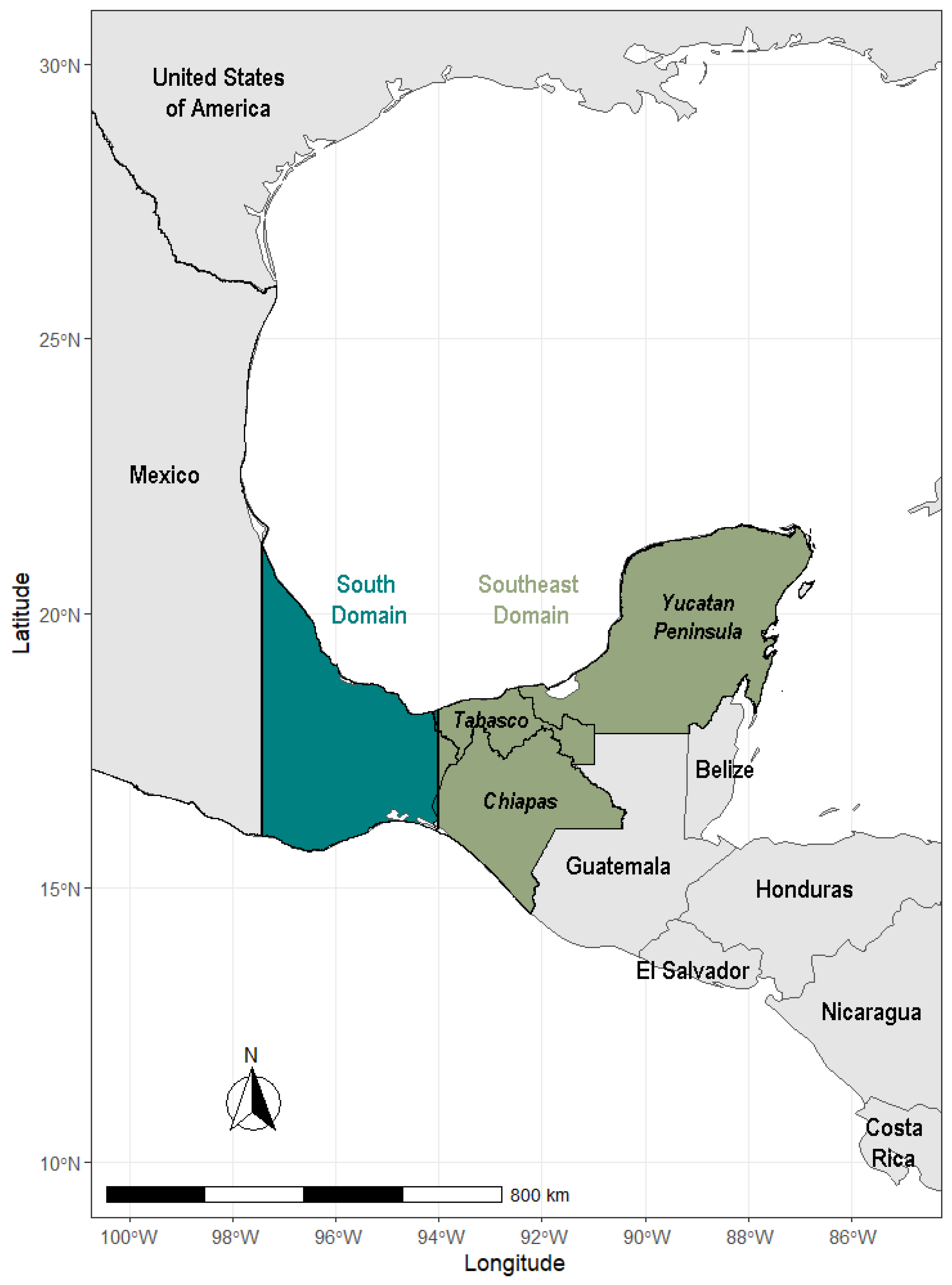
The southern–southeastern region of Mexico (Figure 1) comprises a wide range of climates, from tropical climates to subtropical marine climates, according to a modified version of the Köppen classification [50,51]. It is an area affected by tropical cyclones; in the southern part, these phenomena originate in the Pacific Ocean [52], while in the southeast, it is affected by events in both the Pacific and Atlantic Oceans [53]. Both areas are influenced by cold fronts, but the southeastern zone tends to be more exposed to these phenomena towards the end of the season [54].
The southeastern region is influenced by various meteorological phenomena, notably the Intertropical Convergence Zone (ITCZ) and, indirectly, the Caribbean Low-Level Jet (CLLJ) [55]. Notably, precipitation patterns exhibit distinctive behavior between May and November, marked by the mid-summer drought (MSD), a phenomenon explored by [56].
Regarding annual precipitation levels, the southeast region, encompassing the Grijalva–Usumacinta basin, received an average of 2500 to 2880 mm of rainfall for the period spanning 1960 to 2016 [57]. In contrast, the southern region experienced lower annual precipitation, averaging approximately 1000 to 1300 mm from 1950 to 2010 [51]. This distinction underscores the southeast region’s relatively higher moisture content compared to the southern region [58].
Furthermore, the research of ref. [23] delved into temperature trends in both regions, revealing remarkable similarities. Any deviations in these trends may be attributed to the greater altitude gradient present in the southern region compared to the southeast, further elucidating the complexity of climatic influences in these areas.
The southern–southeastern zone is affected by El Niño-Southern Oscillation (ENSO), the Atlantic Multidecadal Oscillation (AMO), and the Pacific Decadal Oscillation (PDO), according to refs. [58,59]. Environmentally, the zone contains significant ecological reserves [60]. Its approach to natural resource management and indigenous traditions allows for sustainable development. However, it is being impacted by major government projects, such as the Tren Maya and the Isthmus of Tehuantepec Interoceanic Corridor [61].
Socially, the area faces significant disparities and inequalities [62]. Hence, these projects aim to promote regional development in the southern–southeastern region [63,64]. The socioeconomic conditions in this area match the characteristics of the SSP4-6 scenario [65]. The authors of that paper conducted a study using the average temperature variable to determine the CMIP6 scenario. They also conducted a similar exercise using CMIP5.
The southern region of the study area holds significance in the CORDEX-FPS pilot project titled “North America: Dynamical Downscaling Experiments and Hydrological Modeling for Canada and Mexico.” This project aims to conduct thorough investigations and hydrological modeling in Canada and Mexico (For more details, refer to: https://cordex.org/experiment-guidelines/flagship-pilot-studies/endorsed-cordex-flagship-pilote-studies/north-america-dynamical-downscaling-experiments-and-hydrological-modelling-for-canada-and-mexico/, accessed on 21 August 2023).
2.2. Statistical Downscaling
There are different statistical downscaling techniques available, such as perfect prognosis and model output statistics, for example [66]. When dealing with the precipitation variable, quantile mapping methods are commonly employed [20,22,66,67]. For this study, we have chosen to perform bias correction using linear quantile mapping, following the approach of ref. [22]. The correction was applied using the equation proposed by [46]:
where is the inverse cumulative distribution function (CDF), and τ denotes the percentile between 0 and 1. This method assumes a linear relationship between the quantile functionals of the ERA5 data (era5) and the models in the historical period (modh), where and are the coefficients of the linear fit by the regression of least squares. Subsequently, the bias correction is applied for a given time t with the following equation:
To measure the performance of the bias correction, we used the root-mean-square deviation (rmsd), the normalized standard deviation (NSD), the bias in percentage, and the Pearson correlation coefficient. The rmsd is defined here as
where is the precipitation variable, era5 is ERA5 observations, and mod is the model historical data. The NSD is
where σ is the standard deviation for the historical model (modh) and ERA5 (era5). The bias in percentage is
where is the mean precipitation of the model in the historical period, and is the mean precipitation of ERA5. Finally, the Pearson correlation coefficient is
where cov is the covariance of both and , and σ is the standard deviation.
To represent the measurements, we used Taylor’s diagram [68] (Taylor, 2001). These types of diagrams summarize statistical information for evaluating complex models, i.e., correlation, average square-root difference, and the NSD. In this case, we also represented bias. The simulation models that are well consistent with observations are near the point marked “REF”; these models have a high correlation and a low rmsd. Models that are close to the scoring line will have an NSD equal to 1, i.e., a standard deviation equal to or close to the observed [69].
2.3. Data
In this study, we used the ERA5 database to gather historical daily precipitation data and conducted a comprehensive comparison of four climate models: CNRM-ESM2-6A, IPSL-CM6A-LR, MIROC6, and MRI-ESM2-0. The chosen models were in accordance with the work of ref. [23], and their characteristics are summarized in Table 1.
To ensure consistency and facilitate analysis, we interpolated the data onto a 0.25° × 0.25° grid (the same as ERA5). Subsequently, we applied the bias-correction methodology outlined in Section 2.2 to enhance the reliability of the results.
3. Results
3.1. Linear Adjustment
In our analysis, we conducted linear adjustments to the inverse CDFs for both the climate models and ERA5 dataset during the historical period 1980–2014. To facilitate transparency and reproducibility, we have provided the specific parameters ( and ) for the southern and the southeastern regions in Table 2. These adjustments are essential to ensure consistency and comparability between the model outputs and the observational data from ERA5.
3.2. Bias-Correction Performance
To assess the effectiveness of the bias correction, we employed Equations (3) and (4) as performance metrics. The rmsd and the NSD values for the southern and southeastern regions are depicted in Figure 2, Figure 3, Figure 4 and Figure 5.
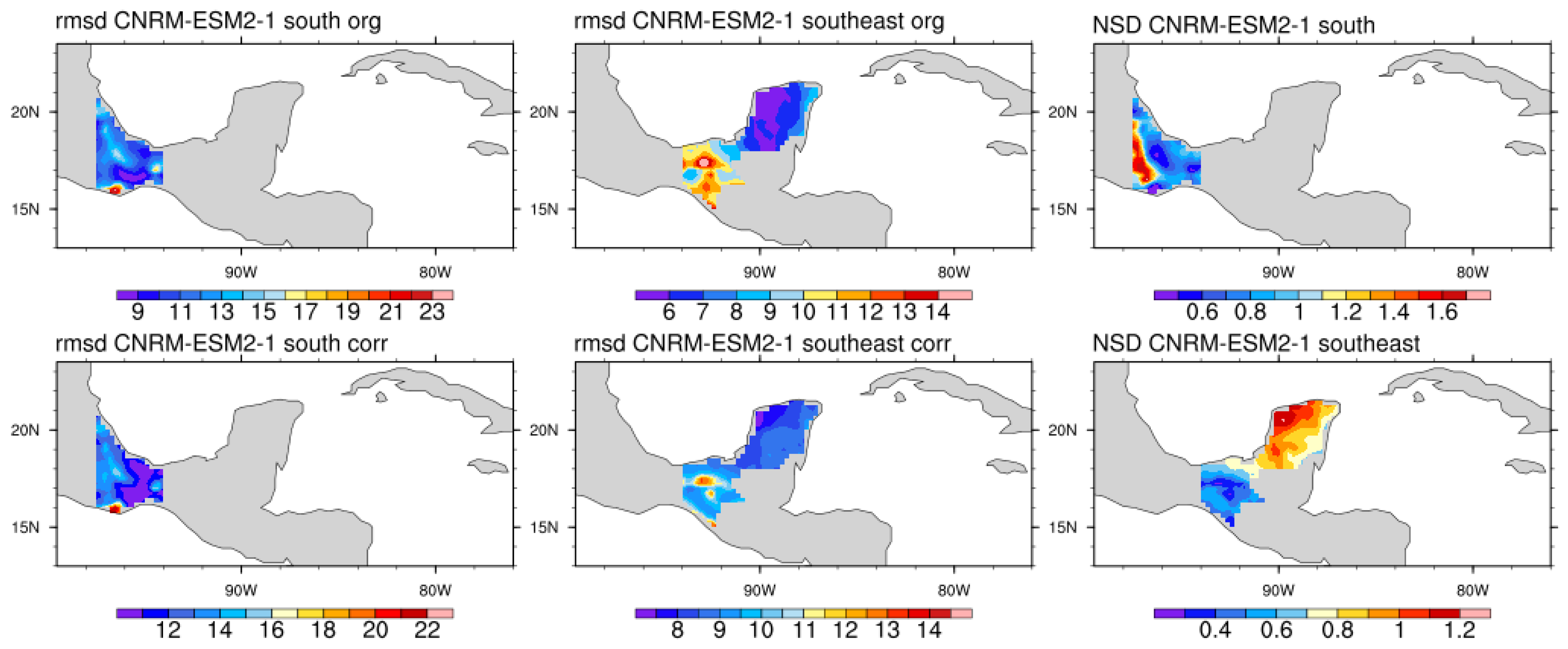
First, we observed that the degree of improvement through bias correction varied depending on the model. For instance, with the CNRM-ESM2-1 model (Figure 2), the rmsd values for the southern region fluctuated between 0 and 23 mm/d, and for the southeastern region, they ranged from 0 to 14 mm/d. A dispersion of rmsd values was observed depending on the grid point (Figure 2). That is why the arial average rmsd was obtained (see Table 3). We will talk about this later. These results indicate a notable improvement in the performance of the CNRM-ESM2-1 model after applying bias correction for both regions.
Overall, the bias correction demonstrated significant improvements in the model’s accuracy, especially for the CNRM-ESM2-1 model, in both the southern and southeastern regions.
In the analysis of the NSD, interesting patterns emerged for different regions. For the southern region, we observed a smaller range of dispersion between values compared to the central and eastern parts, but the western part exhibited a much greater dispersion, with values exceeding 1. This significant dispersion in the western part can be attributed to its proximity to surrounding mountain ranges, which likely influenced the climate dynamics.
Focusing on the southeastern region, we found that the Yucatan peninsula showed a higher dispersion than expected (~1.2), indicating greater variability in its climate. Conversely, the state of Chiapas displayed a much lower dispersion in the model than what was observed (~0.7). It is worth noting that the state of Chiapas experiences notable orographic changes, contributing to its climate’s substantial variability. In contrast, the relief of the Yucatan Peninsula and the state of Tabasco remained relatively stable, and thus, their dispersions are not as significant.
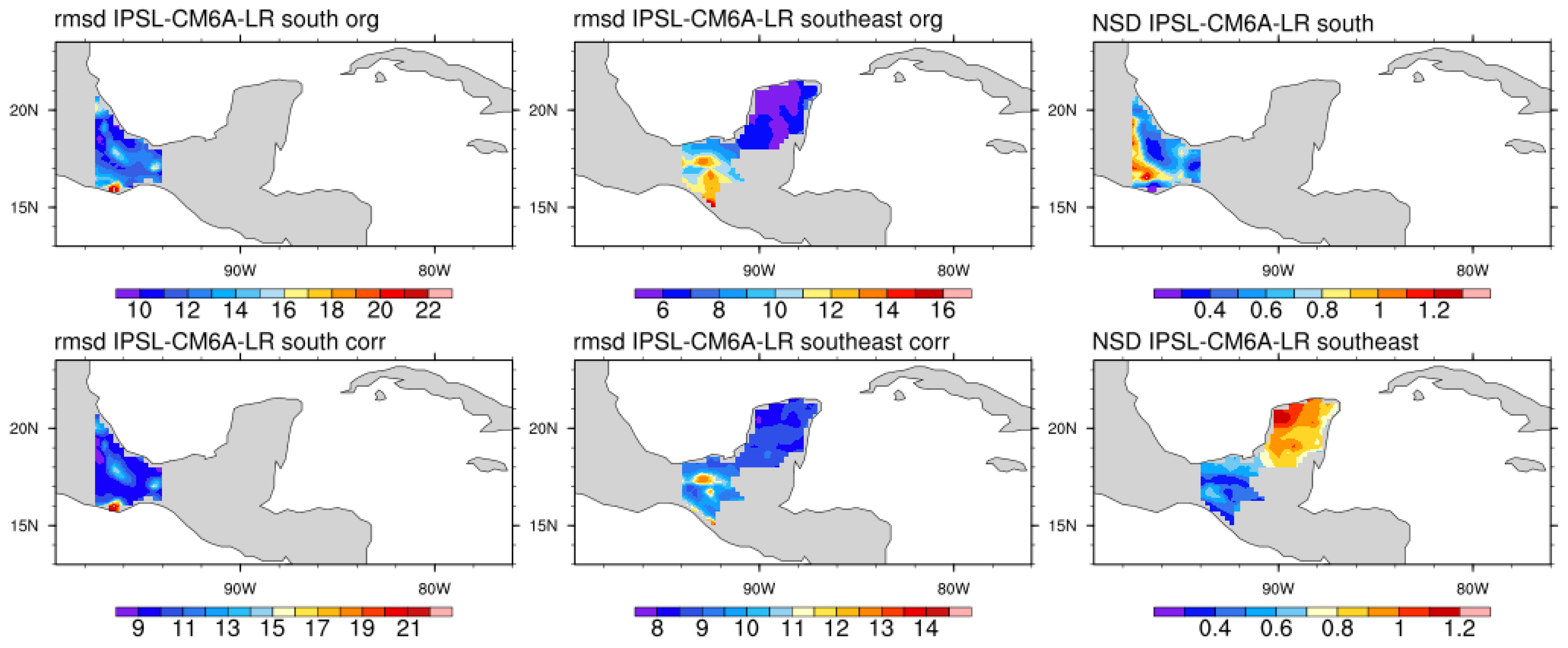
Moreover, the influence of orographic factors on local precipitation becomes evident. The orographic component seems to play a role in shaping the patterns observed in the southern region, as indicated by the IPSL-CM6A-LR model (Figure 3). Similarly, the CNRM-ESM2-1 model showed a comparable signal of the orographic component for the southern region.
When examining the IPSL-CM6A-LR model, we found that its rmsd was also higher for the southern region, ranging from 0 to 22 mm/d, whereas the southeast region exhibited an rmsd range of 0 to 18 mm/d. Applying bias correction to the model data improved the rmsd, which highlights the importance of addressing biases in climate modeling.
For Tabasco and Chiapas, the dispersions of the model with respect to the observations were less than 1 (range 0.4 to 0.8), which suggests a reasonably good fit with the observed values, while for the Yucatan peninsula, values greater than 1 were observed (range from 0.8 to 1.3).
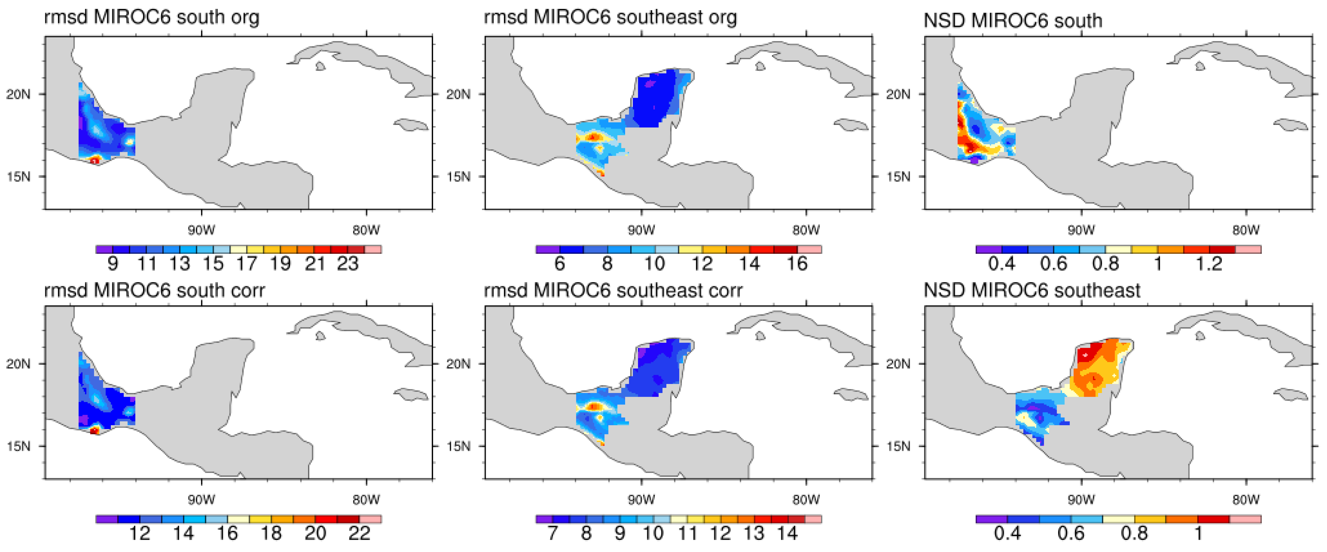
In the context of the MIROC6 model (Figure 4), the rmsd for the southern region exhibited a range of 0 to 24 mm/d, while for the southeast region, it ranged from 0 to 14 mm/d. We observed that applying bias correction to the model data resulted in a slight improvement in rmsd, but significant optimization was not evident.
Regarding the NSD, it is noteworthy that the dispersion of the model was considerably lower than that of the observations, as indicated by values of NSD well below 1. However, despite this difference, the orographic pattern was still evident in the representation of the model in the southern region.
While the southeast region appears distinct, there were variations in the NSD for different areas: for the Yucatan peninsula, the NSD ranged from 0.7 to 1.3, whereas for Tabasco and Chiapas, it ranged from 0.4 to 0.8.
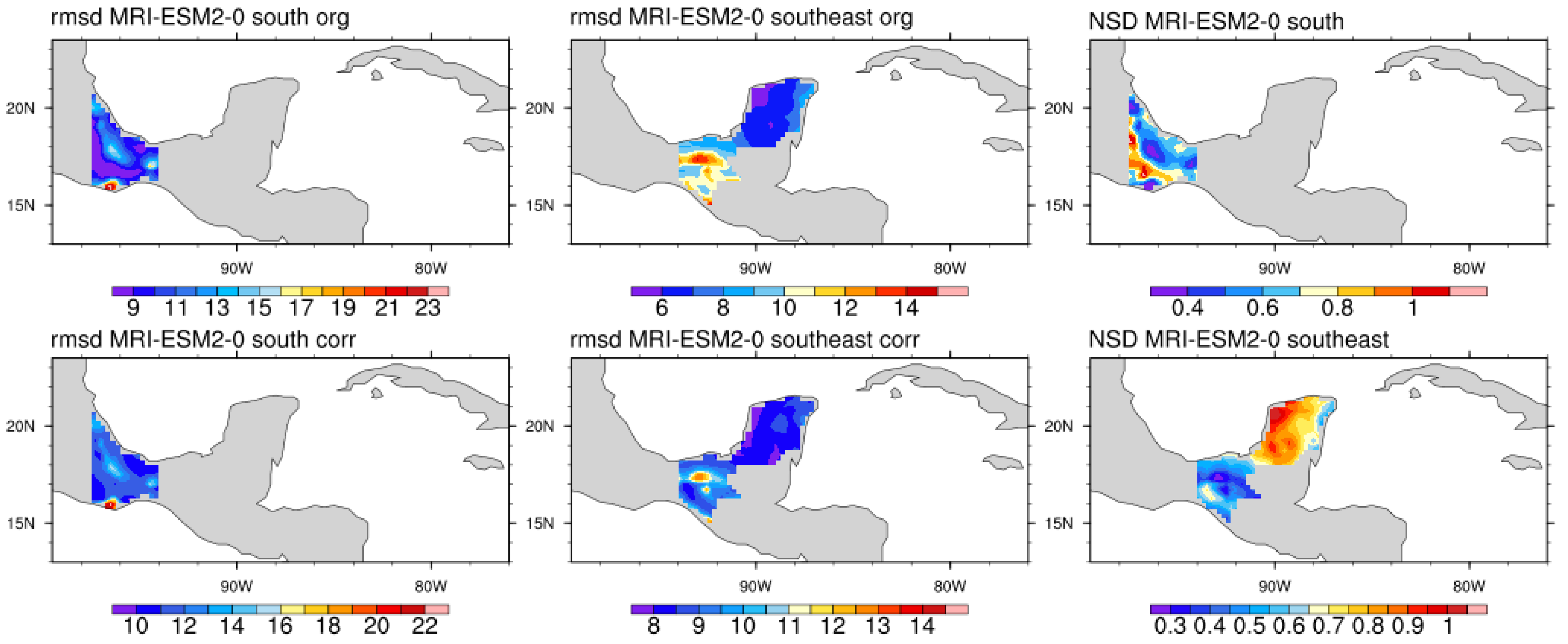
Now, focusing on the MRI-ESM2-0 model (Figure 5), we found that the rmsd for the southeast region showed improvement, particularly in Tabasco and Chiapas, but not for the southern region. The behavior of the NSD in this model was similar to MIROC6, except for the Yucatan peninsula, where its values reached about 1.1.
We have observed that the values of rmsd and NSD not only vary between different climate models but also depend on the specific region under consideration. In order to provide a more comprehensive analysis, we divided the southeast region into two sub-regions: Southeast 1, comprising the states of Tabasco and Chiapas, and Southeast 2, which included the Yucatan Peninsula. To assess the model performance, we calculated the average values for both unbiased and bias-corrected data, as shown in Table 3.
Upon analyzing the results, it becomes evident that bias correction improves the overall signal of the data, particularly for the southern region, followed by the Southeast 1, and the Southeast 2 regions. For the southern region, IPSL-CM6A-LR emerged as the best-performing model with bias correction, followed by CNRM-ESM2-1 and MIROC6.
On the other hand, for the Southeast 1 region, the best bias-corrected model was MIROC6, followed by MRI-ESM2-0 and CNRM-ESM2-1, while for the Southeast 2 region, MIROC6 again was the best model with bias correction, followed by a tie in the performance between CNRM-ESM2-1 and IPSL-CM6A-LR with bias correction.
However, it is crucial to consider the NSD as well, as it indicates the similarity in dispersion with the observed data. When combining the NSD with the rmsd, we found that CNRM-ESM2-1 presented the best overall value for all three regions.
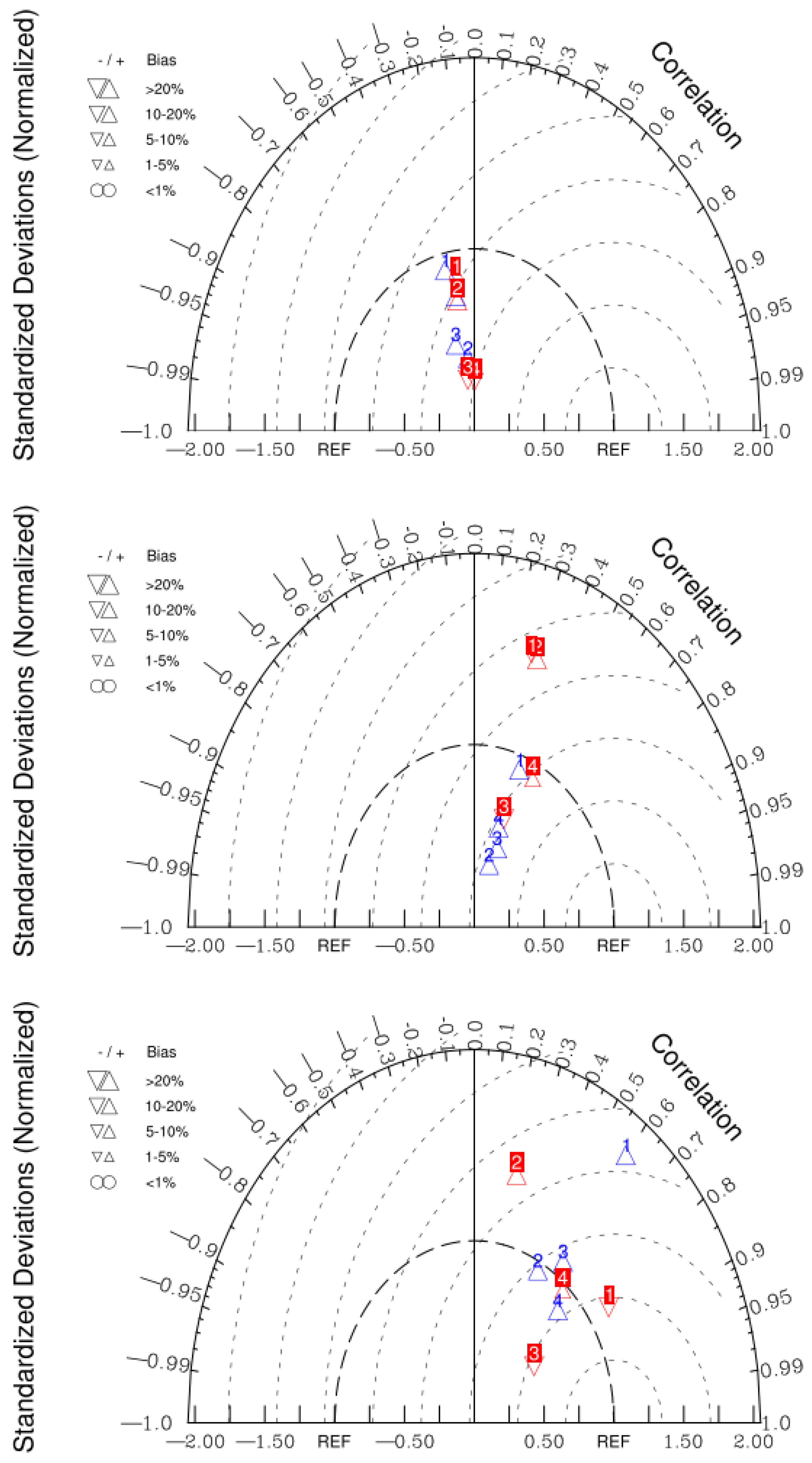
Figure 6 presents the Taylor diagrams for the four models, comparing their performance with and without bias correction. It is evident from all three diagrams that bias correction significantly enhances the performance of the models.
Upon analyzing the Pearson correlation coefficient, we found that the best correlation was observed in the Southeast 2 region, specifically for the Yucatan Peninsula. However, for the south and the Southeast 1 regions, encompassing Tabasco and Chiapas, the correlation was relatively low.
Another important observation is the improvement in the NSD for the south and the Southeast 2 region after bias correction. However, for the Southeast 1 region, although there are changes in the NSD values, the improvement is not as evident as in the other regions.
Regarding the bias itself, we note that after bias correction, all the models exhibited positive values, indicating that they tended to be wetter compared to the original uncorrected data.
4. Discussion and Conclusions
According to the results, bias correction significantly improved the model performance for the study area.
Ref. [70] reported, for the same study area, that the CNRM-ESM2-1 model exhibited a bias of 0.30 mm/day for winter precipitation and 0.28 mm/day for summer precipitation, with a corresponding root-mean-square error (rmse) of 1.47 and 1.56, respectively, for the period 1981–2010. In the study area, model errors ranged between 1 and −1 mm/day for winter and between −2 and −6 mm/day for summer when compared to observations. The application of bias correction resulted in a considerable improvement in rmse, reducing it by almost 50% for the south and approximately 15–25% for the southeast. It is worth noting that the regional error was greater than the worldwide average. CNRM-ESM2-1, being a second-generation model with increased code complexity, physical parameterization, and improved mesh resolution, was reported to exhibit a 10% increase in future processes according to Séférian et al. (2019).
For the IPSL-CM6A-LR model, ref. [71] noted an improvement in simulating precipitation climatology for the south–southeast region of Mexico compared to its CMIP5 version for the period 1980–2005. However, the model tends to globally overestimate precipitation by 0.3 mm/day, which corresponds to 10% of the observed value. In the study area, the NSD was 38% below observations for the south region, 45% below observations for the Southeast 1 region, and 15% below observations for the Southeast 2 region. IPSL-CM6A-LR exhibited improved equilibrium climatic sensitivity, and a better simulation of variables like wind, temperature, and precipitation. Nonetheless, some persisting issues remain, such as the double Intertropical Convergence Zone and the frequency of blocks in winter at medium altitudes.
Ref. [72] showed that the MIROC6 model continued to underestimate global precipitation in the tropical zone, although it was an improvement compared to MIROC5. In the study area, MIROC6 underestimated precipitation in winter for both the south and southeast, while for summer, underestimation was observed only for the south. The NSD values for the study area showed a 25% underestimation for the south, 37% for Southeast 1, and 13% for Southeast 2. MIROC6’s improvements over its predecessor include a new parametrization for convection processes and the inclusion of the stratosphere.
Ref. [73] reported that MRI-ESM2-0 exhibited behavior similar to its predecessor but with an improved correlation of 0.84 compared to 0.79. Globally, MRI-ESM2-0 has a bias of 0.32 mm/day and an rmse of 1.28 mm/day. For the study area, the bias ranged between −1 and −2 mm/day. Like other models, the regional rmse was higher than the global average, exceeding 10 mm/day in the study area. However, applying bias correction reduced this error by up to 50% for the southern region and 15–25% for the southeast. Improvements in MRI-ESM2-0 include a spatial resolution of 100 km, a better redistribution of radiation, and improvements in the parameterization of nonorographic gravitational waves. Nevertheless, the model still presented an overestimation of the temperature during the cooling period from 1950 to 1960.
In summary, the four models showed improvements in the rmsd, of up to 50% for the southern region and between 15 and 25% for the southeast. However, in the case of the NSD and its correlation with ERA5, the best model was CNRM-ESM2-0 for the south and Southeast 1 region. In the Southeast 2 region, this model was last.
Analyzing the diagrams for the southern and the Southeast 1 regions, we observed that IPSL-CM6A-LR and MIROC6 exhibited a strong positive correlation with low rmsd compared to the observations. However, they displayed minimal variability in relation to the observed data. On the other hand, CNRM-ESM2-1 demonstrated a moderate correlation and rmsd difference, aligning closely with the observed variability. Therefore, CNRM-ESM2-1 emerges as the preferred model for these two regions in the southern sector.
Conversely, in the case of the Southeast 2 region, CNRM-ESM2-1 exhibited a notably higher rmsd difference and greater variability compared to the observed data. In contrast, IPSL-CM6A-LR, MIROC6, and MRI-ESM2-0 displaed a strong positive correlation, minimal rmsd difference, and variability patterns that closely resembled the observations. Consequently, these three models emerge as the more suitable choices for modeling the Southeast 2 region.
These results allow us to discriminate between these four models in both the study regions for the future analysis of projections under climate change. This study offers updated information on the use of the MGC of the new generation of CMIP6 for the south–southeast area of Mexico. Finally, it provides a basis for the generation of climate change scenarios in the area for rainfall.
Author Contributions
Conceptualization, M.A.-V.; methodology, M.A.-V.; validation, M.A.-V.; formal analysis, M.A.-V.; investigation, M.A.-V. and M.J.M.-M.; data curation, M.A.-V. and M.J.M.-M.; writing—original draft preparation, M.A.-V. and M.J.M.-M.; writing—review and editing, M.A.-V. and M.J.M.-M.; visualization, M.A.-V. and M.J.M.-M.; supervision, M.A.-V. and M.J.M.-M.; project administration, M.A.-V. and M.J.M.-M.; funding acquisition, M.A.-V. All authors have read and agreed to the published version of the manuscript.
Funding
Cátedra-CONAHCYT under number 945 (M.A.-V.).
Data Availability Statement
We downloaded ERA5 hourly data on individual levels from 1940 and the CMIP6 data from the Climate Data Store to calculate some results presented in this article. We did not download the data for redistribution purposes. We downloaded data from the Climate Data Store on March 2022. Access to the information is available on the site: https://wcrp-cmip.org/cmip-data-access/, accessed on 21 August 2023.
Acknowledgments
We are grateful to the Cátedra-CONAHCYT program, particularly project 945 (M.A.-V.). We also acknowledge CORDEX’s flagship pilot study project “North America: Dynamic Downscaling Experiments and Hydrological Modeling for Canada and Mexico”, its PI José Antonio Salinas-Prieto and María Eugenia Maya-Magaña. We acknowledge the World Climate Research Programme, which, through its Working Group on Coupled Modelling, coordinated and promoted CMIP6. We thank the climate modeling groups for producing and making available their model output, the Earth System Grid Federation (ESGF) for archiving the data and providing access, and the multiple funding agencies who support CMIP6 and ESGF. Finally, we thank the networks of researchers REDESClim and LANRESC to which we belong.
Conflicts of Interest
The authors declare no conflict of interest. The funders had no role in the design of the study; in the collection, analyses, or interpretation of data; in the writing of the manuscript; or in the decision to publish the results.
References
- IPCC. Climate Change 2021: The Physical Science Basis. Contribution of Working Group I to the Sixth Assessment Report of the Intergovernmental Panel on Climate Change; Masson-Delmotte, V.P., Zhai, A., Pirani, S.L., Connors, C., Péan, S., Berger, N., Caud, Y., Chen, L., Goldfarb, M.I., Gomis, M., et al., Eds.; Cambridge University Press: Cambridge, UK; New York, NY, USA, 2021; p. 2391. [Google Scholar] [CrossRef]
- World Meteorological Organization (WMO). 2022. Available online: https://public.wmo.int/en/resources/world-meteorological-day/world-meteorological-day-2022-early-warning-early-action/climate-change-and-extreme-weather (accessed on 21 August 2023).
- Eyring, V.; Bony, S.; Meehl, G.A.; Senior, C.A.; Stevens, B.; Stouffer, R.J.; Taylor, K.E. Overview of the Coupled Model Intercomparison Project Phase 6 (CMIP6) experimental design and organization. Geosci. Model Dev. 2016, 9, 1937–1958. [Google Scholar] [CrossRef]
- Balaji, V.; Taylor, K.E.; Juckes, M.; Lawrence, B.N.; Durack, P.J.; Lautenschlager, M.; Blanton, C.; Cinquini, L.; Denvil, S.; Elkington, M.; et al. Requirements for a global data infrastructure in support of CMIP6. Geosci. Model Dev. 2018, 11, 3659–3680. [Google Scholar] [CrossRef]
- Meinshausen, M.; Vogel, E.; Nauels, A.; Lorbacher, K.; Meinshausen, N.; Etheridge, D.M.; Fraser, P.J.; Montzka, S.A.; Rayner, P.J.; Trudinger, C.M.; et al. Historical greenhouse gas concentrations for climate modelling (CMIP6). Geosci. Model Dev. 2017, 10, 2057–2116. [Google Scholar] [CrossRef]
- Hoesly, R.; O’Rourke, P.; Braun, C.; Feng, L.; Smith, S.J.; Pitkanen, T.; Seibert, J.J.; Vu, L.; Presley, M.; Bolt, R.; et al. Zenodo, Version 23 December 2019, Community Emissions Data System; CERN: Genève, Switzerland, 2019. [Google Scholar] [CrossRef]
- Pascoe, C.; Lawrence, B.N.; Guilyardi, E.; Juckes, M.; Taylor, K.E. Documenting numerical experiments in support of the Coupled Model Intercomparison Project Phase 6 (CMIP6). Geosci. Model Dev. 2020, 13, 2149–2167. [Google Scholar] [CrossRef]
- McGuffie, K.; Henderson-Sellers, A. The Climate Modelling Primer, 4th ed.; Wiley-Blackwell: Chichester, UK, 2014; p. 464. [Google Scholar]
- Fan, X.; Miao, C.; Duan, Q.; Shen, C.; Wu, Y. The performance of CMIP6 versus CMIP5 in simulating temperature extremes over the global land surface. J. Geophys. Res. Atmos. 2020, 125, e2020JD033031. [Google Scholar] [CrossRef]
- Keeble, J.; Hassler, B.; Banerjee, A.; Checa-Garcia, R.; Chiodo, G.; Davis, S.; Eyring, V.; Griffiths, P.T.; Morgenstern, O.; Nowack, P.; et al. Evaluating stratospheric ozone and water vapour changes in CMIP6 models from 1850 to 2100. Atmos. Chem. Phys. 2021, 21, 5015–5061. [Google Scholar] [CrossRef]
- Hirabayashi, Y.; Tanoue, M.; Sasaki, O.; Zhou, X.; Yamazaki, D. Global exposure to flooding from the new CMIP6 climate model projections. Sci. Rep. 2021, 11, 3740. [Google Scholar] [CrossRef]
- Srivastava, A.; Grotjahn, R.; Ullrich, P.A. Evaluation of historical CMIP6 model simulations of extreme precipitation over contiguous US regions. Weather. Clim. Extrem. 2020, 29, 100268. [Google Scholar] [CrossRef]
- Almazroui, M.; Saeed, F.; Saeed, S.; Nazrul Islam, M.; Ismail, M.; Klutse, N.A.B.; Siddiqui, M.H. Projected change in temperature and precipitation over Africa from CMIP6. Earth Syst. Environ. 2020, 4, 455–475. [Google Scholar] [CrossRef]
- Mekonnen, D.G.; Moges, M.A.; Mulat, A.G.; Shumitter, P. The impact of climate change on mean and extreme state of hydrological variables in Megech watershed, Upper Blue Nile Basin, Ethiopia. In Extreme Hydrology and Climate Variability; Elsevier: Amsterdam, The Netherlands, 2019; pp. 123–135. [Google Scholar] [CrossRef]
- Šeparović, L.; Alexandru, A.; Laprise, R.; Martynov, A.; Sushama, L.; Winger, K.; Tete, K.; Valin, M. Present climate and climate change over North America as simulated by the fifth-generation Canadian regional climate model. Clim. Dyn. 2013, 41, 3167–3201. [Google Scholar] [CrossRef]
- Huth, R. Statistical downscaling of daily temperature in central Europe. J. Clim. 2002, 15, 1731–1742. [Google Scholar] [CrossRef]
- Christensen, J.H.; Boberg, F.; Christensen, O.B.; Lucas-Picher, P. On the need for bias correction of regional climate change projections of temperature and precipitation. Geophys. Res. Lett. 2008, 35, L20709. [Google Scholar] [CrossRef]
- Ehret, U.; Zehe, E.; Wulfmeyer, V.; Warrach-Sagi, K.; Liebert, J. HESS Opinions “Should we apply bias correction to global and regional climate model data?”. Hydrol. Earth Syst. Sci. 2012, 16, 3391–3404. [Google Scholar] [CrossRef]
- Maraun, D.; Widmann, M. Statistical Downscaling and Bias Correction for Climate Research; Cambridge University Press: Cambridge, UK, 2018; p. 341. [Google Scholar] [CrossRef]
- Soriano, E.; Mediero, L.; Garijo, C. Selection of Bias Correction Methods to Assess the Impact of Climate Change on Flood Frequency Curves. Water 2019, 11, 2266. [Google Scholar] [CrossRef]
- Bedia, J.; Baño-Medina, J.; Legasa, M.N.; Iturbide, M.; Manzanas, R.; Herrera, S.; Casanueva, A.; San-Martín, D.; Cofiño, A.S.; Gutiérrez, J.M. Statistical downscaling with the downscaleR package (v3.1.0): Contribution to the VALUE intercomparison experiment. Geosci. Model Dev. 2020, 13, 1711–1735. [Google Scholar] [CrossRef]
- Lopez-Cantu, T.; Prein, A.F.; Samaras, C. Uncertainties in future U.S. extreme precipitation from downscaled climate projections. Geophys. Res. Lett. 2020, 47, e2019GL086797. [Google Scholar] [CrossRef]
- Andrade-Velázquez, M.; Montero-Martínez, M.J. Historical and Projected Trends of the Mean Surface Temperature in South-Southeast Mexico Using ERA5 and CMIP6. Climate 2023, 11, 111. [Google Scholar] [CrossRef]
- Wilby, R.L.; Charles, S.P.; Zorita, E.; Timbal, B.; Whetton, P.; Mearns, L.O. Guidelines for Use of Climate Scenarios Developed from Statistical Downscaling Methods. Supporting Material of The Intergovernmental Panel on Climate Change, DDC of IPCC TGCIA, 27, 2004. Available online: https://www.academia.edu/download/31092390/dgm_no2_v1_09_2004.pdf (accessed on 21 August 2023).
- Vrac, M.; Stein, M.; Hayhoe, K. Statistical downscaling of precipitation through nonhomogeneous stochastic weather typing. Clim. Res. 2007, 34, 169–184. [Google Scholar] [CrossRef]
- Tavakolifar, H.; Shahghasemi, E.; Nazif, S. Evaluation of climate change impacts on extreme rainfall events characteristics using a synoptic weather typing-based daily precipitation downscaling model. J. Water Clim. Chang. 2017, 8, 388–411. [Google Scholar] [CrossRef]
- Lee, T.; Singh, V.P. Statistical Downscaling for Hydrological and Environmental Applications; Taylor & Francis Group, LLC.: Boca Raton, FL, USA, 2019; p. 159. [Google Scholar]
- Hewitson, B.C.; Crane, R.G. Climate downscaling: Techniques and application. Clim. Res. 1996, 7, 85–95. [Google Scholar] [CrossRef]
- Benestad, R.E.; Chen, D.; Hanssen-Bauer, I. Empirical-Statistical Downscaling; World Scientific Publishing Company: Hackensack, NJ, USA, 2008; p. 228. [Google Scholar] [CrossRef]
- Jakob Themeßl, M.; Gobiet, A.; Leuprecht, A. Empirical-statistical downscaling and error correction of daily precipitation from regional climate models. Int. J. Climatol. 2011, 31, 1530–1544. [Google Scholar] [CrossRef]
- Hewitson, B.C.; Daron, J.; Crane, R.G.; Zermoglio, M.F.; Jack, C. Interrogating empirical-statistical downscaling. Clim. Chang. 2014, 122, 539–554. [Google Scholar] [CrossRef]
- Wilks, D.S. Adapting stochastic weather generation algorithms for climate change studies. Clim. Chang. 1992, 22, 67–84. [Google Scholar] [CrossRef]
- Rozoff, C.M.; Alessandrini, S. A Comparison between Analog Ensemble and Convolutional Neural Network Empirical-Statistical Downscaling Techniques for Reconstructing High-Resolution Near-Surface Wind. Energies 2022, 15, 1718. [Google Scholar] [CrossRef]
- Cawley, G.C.; Janacek, G.J.; Haylock, M.R.; Dorling, S.R. Predictive uncertainty in environmental modelling. Neural Netw. 2007, 20, 537–549. [Google Scholar] [CrossRef]
- Karamouz, M.; Falahi, M.; Nazif, S.; Rahimi Farahani, M. Long lead rainfall prediction using statistical downscaling and artificial neural network modeling. Trans. A Civ. Eng. 2009, 16, 165–172. Available online: https://www.sid.ir/EN/VEWSSID/J_pdf/95520092A07.pdf (accessed on 21 August 2023).
- Laddimath, R.S.; Patil, N.S. Artificial Neural Network Technique for Statistical Downscaling of Global Climate Model. MAPAN 2019, 34, 121–127. [Google Scholar] [CrossRef]
- Chaudhuri, C.; Robertson, C. CliGAN: A Structurally Sensitive Convolutional Neural Network Model for Statistical Downscaling of Precipitation from Multi-Model Ensembles. Water 2020, 12, 3353. [Google Scholar] [CrossRef]
- Hosseini Baghanam, A.; Norouzi, E.; Nourani, V. Wavelet-based predictor screening for statistical downscaling of precipitation and temperature using the artificial neural network method. Hydrol. Res. 2022, 53, 385–406. [Google Scholar] [CrossRef]
- Hempel, S.; Frieler, K.; Warszawski, L.; Schewe, J.; Piontek, F. A trend-preserving bias correction–the ISI-MIP approach. Earth Syst. Dyn. 2013, 4, 219–236. [Google Scholar] [CrossRef]
- Li, C.; Sinha, E.; Horton, D.E.; Diffenbaugh, N.S.; Michalak, A.M. Joint bias correction of temperature and precipitation in climate model simulations. J. Geophys. Res.-Atmos. 2014, 119, 13–153. [Google Scholar] [CrossRef]
- Cannon, A.J.; Sobie, S.R.; Murdock, T.Q. Bias correction of GCM precipitation by quantile mapping: How well do methods preserve changes in quantiles and extremes? J. Clim. 2015, 28, 6938–6959. [Google Scholar] [CrossRef]
- Mehrotra, R.; Sharma, A. A Multivariate Quantile-Matching Bias Correction Approach with Auto- and Cross-Dependence across Multiple Time Scales: Implications for Downscaling. J. Clim. 2016, 29, 3519–3539. [Google Scholar] [CrossRef]
- Gupta, R.; Bhattarai, R.; Mishra, A. Development of Climate Data Bias Corrector (CDBC) Tool and Its Application over the Agro-Ecological Zones of India. Water 2019, 11, 1102. [Google Scholar] [CrossRef]
- Jaiswal, R.; Mall, R.K.; Singh, N.; Lakshmi Kumar, T.V.; Niyogi, D. Evaluation of bias correction methods for regional climate models: Downscaled rainfall analysis over diverse agroclimatic zones of India. Earth Space Sci. 2022, 9, e2021EA001981. [Google Scholar] [CrossRef]
- Ines, A.V.; Hansen, J.W. Bias correction of daily GCM rainfall for crop simulation studies. Agric. For. Meteorol. 2006, 138, 44–53. [Google Scholar] [CrossRef]
- Qian, W.; Chang, H.H. Projecting Health Impacts of Future Temperature: A Comparison of Quantile-Mapping Bias-Correction Methods. Int. J. Environ. Res. Public Health 2021, 18, 1992. [Google Scholar] [CrossRef]
- Wehner, M.; Easterling, D.R.; Lawrimore, J.H.; Heim, R.R.; Vose, R.S.; Santer, B.D. Projections of future drought in the continental United States and Mexico. J. Hydrometeorol. 2011, 12, 1359–1377. [Google Scholar] [CrossRef]
- Mendez, M.; Maathuis, B.; Hein-Griggs, D.; Alvarado-Gamboa, L.F. Performance evaluation of bias correction methods for climate change monthly precipitation projections over Costa Rica. Water 2020, 12, 482. [Google Scholar] [CrossRef]
- Hersbach, H.; Bell, B.; Berrisford, P.; Biavati, G.; Horányi, A.; Muñoz Sabater, J.; Nicolas, J.; Peubey, C.; Radu, R.; Rozum, I.; et al. ERA5 Hourly Data on Pressure Levels from 1940 to Present. Copernicus Climate Change Service (C3S) Climate Data Store (CDS). 2023. Available online: https://cds.climate.copernicus.eu/cdsapp#!/dataset/10.24381/cds.bd0915c6?tab=overview (accessed on 21 August 2023). [CrossRef]
- García, E. Modificaciones al Sistema de Clasificación Climática de Köppen (Para Adaptarlo a Las Condiciones de La República Mexicana, 5th ed.; Instituto de Geografía, UNAM: Ciudad de México, México, 2004; Available online: http://www.publicaciones.igg.unam.mx/index.php/ig/catalog/book/83 (accessed on 21 August 2023).
- Fideicomiso para el Desarrollo Regional del Sur Sureste (FIDESUR). Estrategia Nacional para el Desarrollo Integral de la región Sur Sureste (ENDIRSSE). 2021. Available online: https://sursureste.org.mx/sites/default/files/ENDRSSE-2-RSSE-y-contexto-geografico-v1.pdf (accessed on 1 September 2023).
- Dominguez, C.; Jaramillo, A.; Cuéllar, P. Are the socioeconomic impacts associated with tropical cyclones in Mexico exacerbated by local vulnerability and ENSO conditions? Int. J. Climatol. 2021, 41, E3307–E3324. [Google Scholar] [CrossRef]
- Andrade-Velázquez, M. Visión climática de la precipitación en la cuenca del Río Usumacinta. In La Cuenca del Río Usumacinta desde la Perspectiva del Cambio Climático; Soares, D., García, G.A., Eds.; Instituto Mexicano de Tecnología del Agua: Jiutepec, México, 2017; pp. 1–417. [Google Scholar]
- Magaña, V.; Vázquez, J.L.; Pérez, J.L.; Pérez, J.B. Impact of El Niño on precipitation in Mexico. Geofis. Int. 2003, 42, 313–330. [Google Scholar] [CrossRef]
- Sáenz, F.; Hidalgo, H.G.; Muñoz, Á.G.; Alfaro, E.J.; Amador, J.A.; Vázquez-Aguirre, J.L. Atmospheric circulation types controlling rainfall in the Central American Isthmus. Int. J. Climatol. 2023, 43, 197–218. [Google Scholar] [CrossRef]
- Straffon, A.; Zavala-Hidalgo, J.; Estrada, F. Preconditioning of the precipitation interannual variability in southern Mexico and Central America by oceanic and atmospheric anomalies. Int. J. Climatol. 2020, 40, 3906–3921. [Google Scholar] [CrossRef]
- Andrade-Velázquez, M.; Medrano-Pérez, O.R. Precipitation patterns in Usumacinta and Grijalva basins (southern Mexico) under a changing climate. Rev. Bio Cienc. 2020, 7, 1–22. [Google Scholar] [CrossRef]
- INEGI. Cuentame, Información por Entidad. Instituto Nacional de Estadística y Geografía. 2023. Available online: https://cuentame.inegi.org.mx/monografias/default.aspx?tema=me (accessed on 1 September 2023).
- Andrade-Velázquez, M.; Medrano-Pérez, O.R. Historical precipitation patterns in the South-Southeast region of Mexico and future projections. Earth Sci. Res. J. 2021, 25, 69–84. [Google Scholar] [CrossRef]
- Comisión Nacional para el Conocimiento y Uso de la Biodiversidad (CONABIO). “Atlas de naturaleza y Sociedad”. CONABIO, México, D.F. Atlas de Naturaleza y Sociedad. 2015. Available online: https://www.biodiversidad.gob.mx/atlas/ (accessed on 21 August 2023).
- Centro Mexicano de Derecho Ambiental, A.C. (CEMDA). Todo lo Que Tienes Que Saber Sobre el Tren Maya. 2023. Available online: https://www.cemda.org.mx/tren-maya/ (accessed on 21 August 2023).
- Kauffer, E. El Agua en la Frontera Sur de México: Una Aproximación a la Problemática de las Cuencas Compartidas Con Guatemala y Belice. Boletín del Archivo Histórico del Agua, no. 33, Año 11, Mayo-Agosto, México, AHA/CIESAS/CNA. 2006. Available online: https://biblat.unam.mx/hevila/Boletindelarchivohistoricodelagua/2006/vol11/no33/3.pdf (accessed on 21 August 2023).
- Tren Maya. Secretaria de Turismo y Fonatur. Gobierno de México. 2023. Available online: https://www.gob.mx/trenmaya (accessed on 21 August 2023).
- Corredor Interoceánico-Istmo de Tehuantepec (CIIT). Gobierno de México. 2023. Available online: https://www.gob.mx/ciit (accessed on 21 August 2023).
- Andrade-Velázquez, M.; Medrano-Pérez, O.R.; Montero-Martínez, M.J.; Alcudia-Aguilar, A. Regional Climate Change in Southeast Mexico-Yucatan Peninsula, Central America and the Caribbean. Appl. Sci. 2021, 11, 8284. [Google Scholar] [CrossRef]
- Bruyère, C.L.; Done, J.M.; Holland, G.J.; Fredrick, S. Bias corrections of global models for regional climate simulations of high-impact weather. Clim. Dynam. 2014, 43, 1847–1856. [Google Scholar] [CrossRef]
- Zhao, T.; Bennett, J.C.; Wang, Q.J.; Schepen, A.; Wood, A.W.; Robertson, D.E.; Ramos, M.H. How suitable is quantile mapping for postprocessing GCM precipitation forecasts? J. Clim. 2017, 30, 3185–3196. [Google Scholar] [CrossRef]
- Taylor, K.E. Summarizing multiple aspects of model performance in a single diagram. J. Geophys. Res. 2001, 106, 7183–7192. [Google Scholar] [CrossRef]
- Taylor, K.E. Taylor Diagram Primer. 2005. Available online: https://pcmdi.llnl.gov/staff/taylor/CV/Taylor_diagram_primer.pdf (accessed on 1 September 2023).
- Séférian, R.; Nabat, P.; Michou, M.; Saint-Martin, D.; Voldoire, A.; Colin, J.; Decharme, B.; Delire, C.; Berthet, S.; Chevallier, M.; et al. Evaluation of CNRM Earth System Model, CNRM-ESM2-1: Role of Earth system processes in present-day and future climate. J. Adv. Model. Earth Syst. 2019, 11, 4182–4227. [Google Scholar] [CrossRef]
- Boucher, O.; Servonnat, J.; Albright, A.L.; Aumont, O.; Balkanski, Y.; Bastrikov, V.; Bekki, S.; Bonnet, R.; Bony, S.; Bopp, L.; et al. Presentation and evaluation of the IPSL-CM6A-LR climate model. J. Adv. Model. Earth Syst. 2020, 12, e2019MS002010. [Google Scholar] [CrossRef]
- Tatebe, H.; Ogura, T.; Nitta, T.; Komuro, Y.; Ogochi, K.; Takemura, T.; Sudo, K.; Sekiguchi, M.; Abe, M.; Saito, F.; et al. Description and basic evaluation of simulated mean state, internal variability, and climate sensitivity in MIROC6. Geosci. Model Dev. 2019, 12, 2727–2765. [Google Scholar] [CrossRef]
- Yukimoto, S.; Kawai, H.; Koshiro, T.; Oshima, N.; Yoshida, K.; Urakawa, S.; Tsujino, H.; Deushi, M.; Tanaka, T.; Hosaka, M.; et al. The Meteorological Research Institute Earth System Model version 2.0, MRI-ESM2. 0: Description and basic evaluation of the physical component. J. Meteorol. Soc. Jpn. Ser. II 2019, 97, 931–965. [Google Scholar] [CrossRef]
Figure 1.
Study area for the southern and southeastern domains of Mexico.

Figure 2.
Original (org) and bias-corrected (corr) rmsd for southern (plots on the left) and southeastern (plots in the middle) Mexico of the CNRM_ESM2-1 model. In addition, the NSD for both southern (plot in the top right) and southeastern Mexico (plot in the bottom right) are shown for the same model.

Figure 3.
The same as in Figure 2 but for the IPSL-CM6A-LR model.
Figure 3.
The same as in Figure 2 but for the IPSL-CM6A-LR model.

Figure 4.
The same as in Figure 2 but for the MIROC6 model.
Figure 4.
The same as in Figure 2 but for the MIROC6 model.

Figure 5.
The same as in Figure 2 but for the MRI-ESM2-0 model.
Figure 5.
The same as in Figure 2 but for the MRI-ESM2-0 model.

Figure 6.
Taylor diagrams comparing the performance of the four models with and without bias correction. Each model is represented by a number: (1) CNRM-ESM2-6A, (2) IPSL-CM6A-LR, (3) MIROC6, and (4) MRI-ESM2-0. The diagrams are presented in blue for the case with bias correction and in red for the case without bias correction. The top diagram relates to the southern region, the middle one to the Southeast 1 region (Tabasco and Chiapas), and the bottom one to the Southeast 2 region(Yucatan Peninsula). The dotted semicircles represent the difference between the rmsd of the model and that of the observations.


Table 1.
Data used for the precipitation () of ERA5 and the historical data of four GCMs in the period 1980–2014 (https://creativecommons.org/licenses /by/4.0/, accessed on 21 August 2023).
Table 1.
Data used for the precipitation () of ERA5 and the historical data of four GCMs in the period 1980–2014 (https://creativecommons.org/licenses /by/4.0/, accessed on 21 August 2023).
| Number | Data | Resolution | Reference |
|---|---|---|---|
| 1 | ERA5 | 25 km × 25 km | [49] |
| 2 | CNRM-ESM2-1 | 250 km × 250 km | [70] |
| 3 | IPSL-CM6A-LR | 250 km × 250 km | [71] |
| 4 | MIROC6 | 250 km × 250 km | [72] |
| 5 | MRI-ESM2-0 | 100 km × 100 km | [73] |
Table 2.
Parameters and of the linear adjustment of quantile mapping [Equation (1)] for the two regions and four models analyzed in this study.
Table 2.
Parameters and of the linear adjustment of quantile mapping [Equation (1)] for the two regions and four models analyzed in this study.
| Number | Data | (South) | (South) | (Southeast) | (Southeast) |
|---|---|---|---|---|---|
| 1 | CNRM-ESM2-1 | 7.743 | 0.762 | 10.609 | 0.281 |
| 2 | IPSL-CM6A-LR | 6.365 | 0.427 | 10.896 | −0.003 |
| 3 | MIROC6 | 15.420 | −0.114 | 9.061 | 0.236 |
| 4 | MRI-ESM2-0 | 12.398 | 0.195 | 9.757 | 0.087 |
Table 3.
The rmsd and NSD values for the four models and the regions in the study area. Note that the southeast was divided into Southeast 1 (Tabasco, Chiapas) and Southeast 2 (Yucatan Peninsula).
Table 3.
The rmsd and NSD values for the four models and the regions in the study area. Note that the southeast was divided into Southeast 1 (Tabasco, Chiapas) and Southeast 2 (Yucatan Peninsula).
| Data | South rmsd Orig | South rmsd Corr | South rmsd Corr/Orig | Southeast 1 rmsd Orig | Southeast 1 rmsd Corr | Southeast 1 rmsd Corr/Orig | Southeast 2 rmsd Orig | Southeast 2 rmsd Corr | Southeast 2 rmsd Corr/Orig |
|---|---|---|---|---|---|---|---|---|---|
| CNRM-ESM2-1 | 12.155 | 6.756 | 0.556 | 12.928 | 9.735 | 0.753 | 9.870 | 8.535 | 0.865 |
| IPSL-CM6A-LR | 12.639 | 6.322 | 0.500 | 10.951 | 9.934 | 0.907 | 10.066 | 8.704 | 0.865 |
| MIROC6 | 12.600 | 7.126 | 0.566 | 12.940 | 9.323 | 0.720 | 9.823 | 7.782 | 0.792 |
| MRI-ESM2-0 | 11.260 | 6.998 | 0.621 | 12.620 | 9.389 | 0.744 | 9.649 | 8.411 | 0.872 |
Disclaimer/Publisher’s Note: The statements, opinions and data contained in all publications are solely those of the individual author(s) and contributor(s) and not of MDPI and/or the editor(s). MDPI and/or the editor(s) disclaim responsibility for any injury to people or property resulting from any ideas, methods, instructions or products referred to in the content. |
© 2023 by the authors. Licensee MDPI, Basel, Switzerland. This article is an open access article distributed under the terms and conditions of the Creative Commons Attribution (CC BY) license (https://creativecommons.org/licenses/by/4.0/).
Share and Cite
MDPI and ACS Style
Andrade-Velázquez, M.; Montero-Martínez, M.J. Statistical Downscaling of Precipitation in the South and Southeast of Mexico. Climate 2023, 11, 186. https://doi.org/10.3390/cli11090186
AMA Style
Andrade-Velázquez M, Montero-Martínez MJ. Statistical Downscaling of Precipitation in the South and Southeast of Mexico. Climate. 2023; 11(9):186. https://doi.org/10.3390/cli11090186
Chicago/Turabian StyleAndrade-Velázquez, Mercedes, and Martín José Montero-Martínez. 2023. "Statistical Downscaling of Precipitation in the South and Southeast of Mexico" Climate 11, no. 9: 186. https://doi.org/10.3390/cli11090186
Note that from the first issue of 2016, this journal uses article numbers instead of page numbers. See further details here.