Artificial Neural Network (ANN)-Based Long-Term Streamflow Forecasting Models Using Climate Indices for Three Tributaries of Goulburn River, Australia

Abstract

Water resources systems planning, and control are significantly influenced by streamflow forecasting. The streamflow in northern and north-central regions of Victoria (Australia) is influenced by different climate indices, such as El Niño Southern Oscillation, Interdecadal Pacific Oscillation, Pacific Decadal Oscillation, and Indian Ocean Dipole. This paper presents the development of the ANN model using machine learning with the multi-layer perceptron and Levenberg algorithm for long-term streamflow forecasting for three tributaries of Goulburn River located within Victoria through establishing relationships between climate indices and streamflow. The climate indices were used as input predictors and the models’ performances were analyzed through best fit correlation. The higher correlation values of the developed models evident from Pearson regression (R) values ranging from 0.61 to 0.95 reveal the models’ acceptability. The accuracies of ANN models were evaluated using statistical measures such as Root Mean Square Error (RMSE), Mean Absolute Error (MAE) and Mean Absolute Percentage Error (MAPE). It is found that considering R, RMSE, MAE and MAPE values, the ENSO has more influence (61% to 95%) on the streamflow of Goulburn River tributaries than other climate drivers. Moreover, it is concluded that Acheron ANN models are the best models that can be confidently used to forecast the streamflow even six-months ahead.

1. Introduction

The climate, geology and topography are the primary characteristics of streams or basins affecting streamflow. The streamflow is mostly affected by climate change, i.e., rainfall, droughts, atmosphere, as well as an increase in population. The increase in population directly increases the water demands for irrigation and water supply systems. The streamflow is a very important factor within long-term hydrologic variability, and the effect of climate change has been altering this variable. The knowledge of variability and trend of streamflow is important for water resource management and planning purposes [1]. The main sources of streamflow forecasting are initial catchment conditions (preceding streamflow, preceding rainfall and soil moisture levels of groundwater) and climate variables or climate drivers [2]. The large-scale climate indices or drivers have major influence on the streamflow and rainfall because the climate indices fluctuate at very low frequencies [3,4]. Australia is encircled by the Pacific, Indian, and Southern Oceans and is influenced by the climatic anomalies arising from these Oceans. The spatial and temporal variations take place in climate drivers containing sea surface temperature and sea level pressure anomalies. Furthermore, it is very difficult to integrate the initial conditions of catchments to develop streamflow forecasting models. The south-east Australian climate is influenced by five major climate drivers, i.e., El-Niño Southern Oscillation (ENSO), Interdecadal Pacific Oscillation (IPO), Pacific Decadal Oscillation (PDO), Southern Annual Mode (SAM) and Indian Ocean Dipole (IOD), which are originating from the Pacific, Indian, and Southern Oceans. These oceans have a large impact on the climate of south-east Australia [5]. El-Niño Sothern Oscillation is the natural cycle in the Pacific Ocean’s temperature, cloud, and winds. It is the leading interannual climate variability around the globe. It plays an important role in global climate prediction. The El-Niño southern oscillation affects the sea surface temperature (SST) and air pressure (A.P) over the streamflow. It also affects the dynamics of atmosphere and ocean worldwide [5,6,7]. The climate conditions vary due to La Nina and El-Niño events around the Pacific, including eastern Australia [8]. The ENSO events have a significant impact on the climate of different countries around the world, i.e., Japan, New Zealand, western coast of United states, Australia, and South China [6,9,10,11]. Furthermore, ENSO and IOD have large-scale climate effects on India, Australia, and North and South America. Several researchers observed the effect of climate drivers on the streamflow and rainfall of Australia [12,13,14]. It is to be noted that due to numerous studies involving these indices, it apparently seems that these indices are the main drivers of the rainfall occurrences. In reality, these are not the main drivers, rather just some measures of selective atmospheric variables. The main drivers of the rainfall are complex ocean–atmospheric interactions, explanations of which are beyond the scope of this study.

The IOD is an atmospheric phenomenon similar to ENSO. It is evolved in the Indian Ocean on an inter-annual time scale. The rainfall in Murray Darling Basin (MDB), Australia, is affected due to IOD from the months of June to November. The IOD is the key climate driver of Australia because of its significant influence in Australian agriculture [15]. The IOD events have significant influences on the growing crops in winter season in the region. The events generally start in the month of May or June and remain at their peak between August and October; after this point, they quickly slow towards the end of spring, when monsoons reach the southern hemisphere [16,17]. The ENSO is causing interannual variability in Australian rainfall and streamflow. Many authors showed the impact of ENSO on streamflow and revealed that seasonal (spring) streamflow and rainfall can be predicted by ENSO anomalies [6,18]. Moreover, a few researchers have showed the significant impact of IPO on streamflow and rainfall variation on a decadal to multidecadal time scale. It can increase or decrease the flood risks in New South Wales (NSW), Australia [4,19]. The correlation of the lagged ENSO-streamflow data set can be used to develop seasonal streamflow forecasting models. The seasonal rainfall and streamflow forecasting is important for the land and water resources management [18]. An earlier study found that the Bayesian Joint probability modeling technique that used ENSO-SST indices shows close correlation with higher lagged months. Whereas the indices from Indian and extratropical regions or derivatives from atmospheric indices such as PDO and IOD tend to show the good correlation only for one-month lag and with the increase in lag months, the correlation between streamflow and climate indices is becoming weak [20]. This supports the view that the PDO-Niño3.4, in combination, can be used for spring streamflow forecasting, with Pearson regression (R) ranging from 0.25 to 0.45 [6]. In addition to this, the influences of ENSO and IOD were analyzed on Victorian rainfall, and the study concluded that ENSO and IOD have more influence on spring rainfall [21]. Moreover, ENSO and IOD also have shown the inclusive influence on the rainfall and streamflow of NSW, but it is observed that the IPO indices do not have much influence on the rainfall of NSW [5]. Furthermore, it is investigated that PDO is not showing a good correlation with seasonal streamflow of some stations of NSW, where correlations ranged from 0.20 to 0.25 [6]. A study determined the relationship of seasonal streamflow to a reservoir in Sydney and individual Niño3.4 and PDO indices and revealed regression (R) values of −0.17 and −0.19, respectively [22]. On other hand, a study has shown a greater positive impact of PDO on the annual rainfall of Sydney in comparison to SOI [23]. In addition to this, another study also showed the significant relationship between PDO and Australian summer monsoon but not for NSW [12].

Artificial Intelligence and machine learning techniques, such as extreme machine learning, the fuzzy neural network model, the artificial neural network, wavelet, discrete wavelet transform, Empirical Mode Decomposition (EMD), hybrid DWT, EMD-ANN models, the regression model, M5 model tree, and Vector Support Machine (SVM), have been extensively used for the last 15 years to resolve various water resources issues and environment-related problems [14,24]. Nowadays, the artificial neural network is widely used for hydrological modeling and its applications for predicting and forecasting the streamflow [25,26,27,28,29], rainfall-runoff modeling [30], ground water level forecasting [31], and evapotranspiration estimations [32,33].

For the study of trend and variability analysis, it is important to understand the behavior of hydrological and climate variables over a long-term period. The oscillation modes on temporal pattern in the time series of climate variation were analyzed by exploratory analysis on raw data, and their structure and properties and quasi-periodic behavior were determined by wavelet analysis [7]. In their study, the authors improved the wavelet modeling framework for hydrological time series forecasting, which was found to be more useful [34]. Various researchers used the hourly, daily, weekly, and seasonal streamflow data to find the suitable variables for streamflow and rainfall forecasting [2,35,36], and many others [12,13,14] have investigated the synchronized relation of a single climate variable with daily, monthly, or seasonal streamflow and rainfall and revealed that the climate indices have an impact on the streamflow of Australia. Contrastingly, very limited researchers have developed a monthly streamflow relationship in different parts of Australia [37], and no one has explored the teleconnection between continuous monthly streamflow and climate indices of the studied rivers, especially within Australia. To further improve the monthly forecasting capability, this research was carried out to establish teleconnections between ENSO, IPO, PDO, and IOD indices and monthly streamflow. The paper describes the long-term streamflow forecasting outcomes performed on three tributaries of Goulburn River within MDB using continuous monthly streamflow and climate drivers as input data for different ANN models.

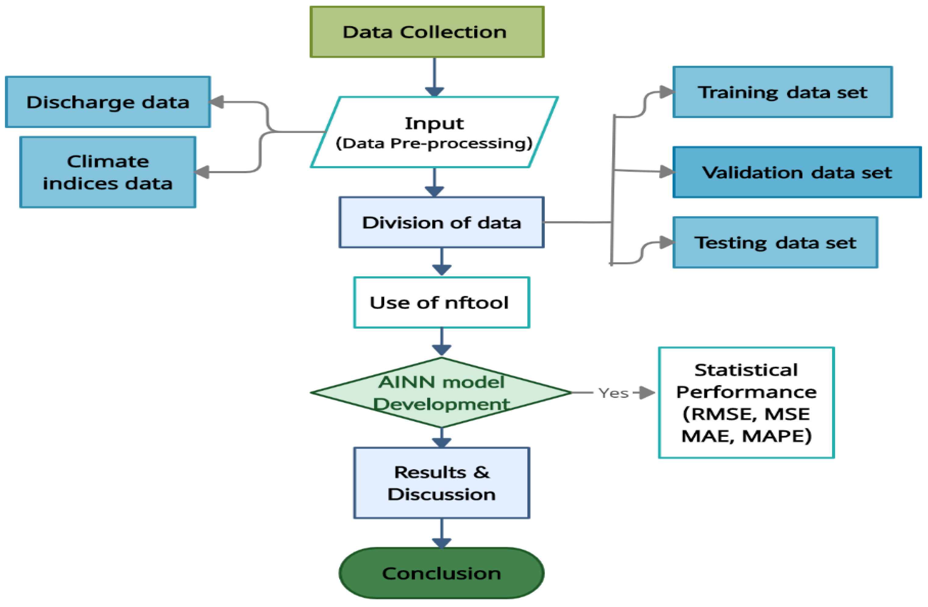
2. Materials and Methods

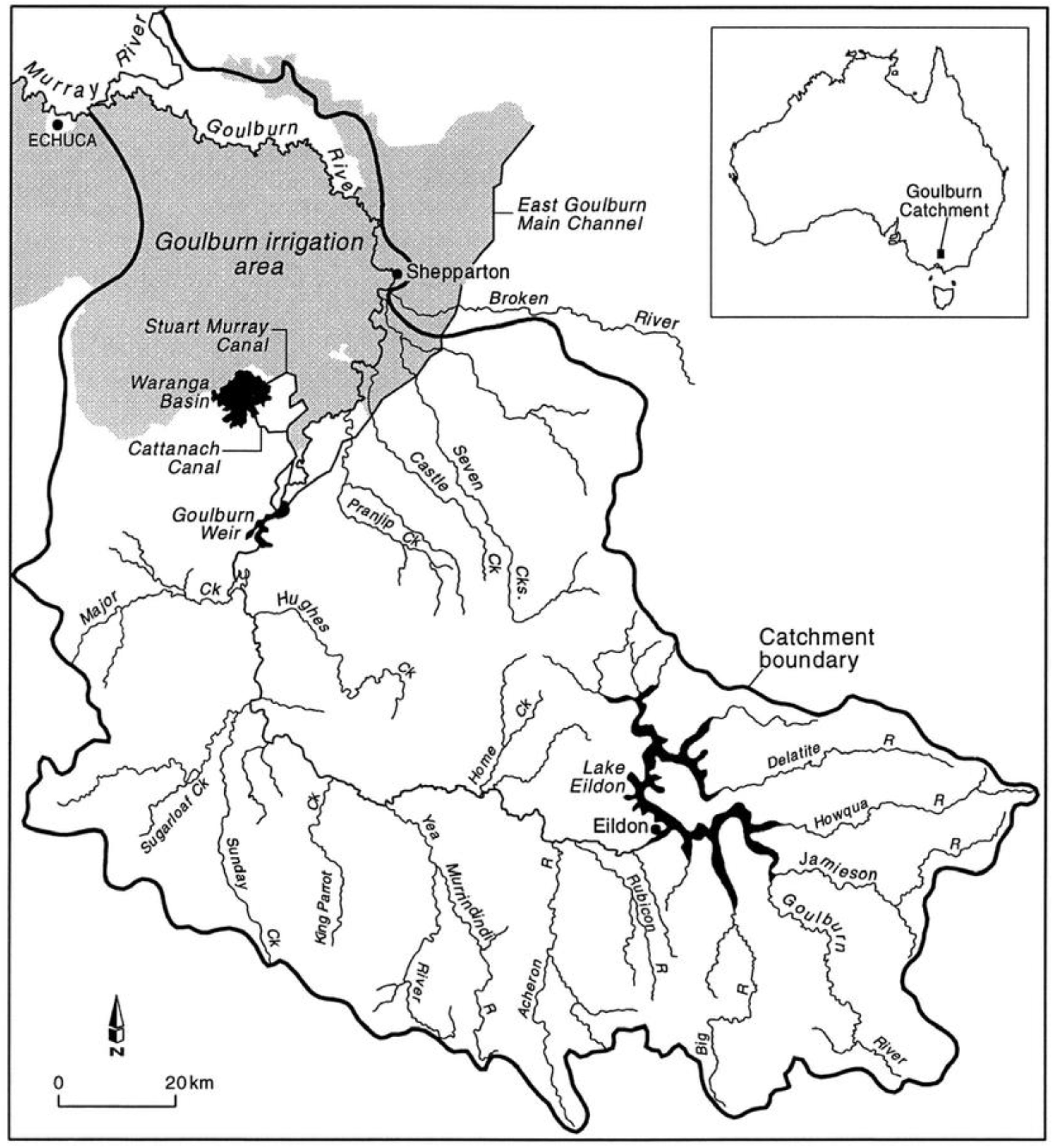
2.1. Study Area

For this study, three tributaries of Goulburn River (37°32′–38°9′ S, 145°2′–146°11′ E) were selected because of its prominence within Goulburn Broken catchment in the state of Victoria (Figure 1). The Australian economy heavily depends on farming products irrigated nearby in the Murray–Darling Basin (MDB), and the MDB contributes AUD 24 billion in food and fiber per year. It contributes approximately 40% of agricultural production and irrigates 65% of the land in Australia [38]. The Goulburn is 654 km long and flows into Murray River, the largest river of Australia. It is rich with environmental, cultural, and recreational values and flows in the western direction, across a widespread agriculture valley. The Goulburn River is used for multiple purposes, including supplies for the irrigation, for water supply to the small towns and for ecological outcomes [15,16]. The Goulburn River is fed by high annual rainfall and snow melt on average 63 inches from mountains. The Goulburn River catchment climate is pleasant and semi-arid. The monthly mean maximum temperature of catchment in the summer season is around 30 °C and in winter is 14 °C, whereas the monthly mean minimum temperature ranges from around 14 to 2 °C. In this study, two regions of Victoria have been selected: one is north-central and the other is northern. The three stations that have been selected from the north-central region are Acheron, Rubicon, and Yea; Goulburn station was selected from the northern region [16,39,40,41]. These rivers are at the downstream of Hume reservoir and mostly serve agricultural and irrigation purposes for the yield production [16].

2.2. Data Description

The aim of this study is to analyze the correlation between streamflow and climate drivers using machine learning techniques to predict and forecast the streamflow of Goulburn River and its main tributaries. In this study, streamflow and climate indices data over the last 48 years (1974 to 2022) were used. Additionally, the data set was distributed as 15% for the training period, 15% for the validation period and 70% for the testing period. The simulation results are from the testing period. The mean discharge data in cumec (m³/s) were used to balance the missing values. The historical monthly streamflow data of selected stations were collected from different websites, the details of which are given in

Table 1. Overview of the selected discharge stations [16,42].

Station No.	Latitude	Longitude	River Name & Data Source
405209	37.32° S	145.71° E	Acheron River at Taggerty https://realtimedata.waternsw.com.au/ # https://data.water.vic.gov.au/static.htm #
405217	37.38° S	145.47° E	Yea River at Devlins Bridge https://data.water.vic.gov.au/static.htm #
405241	37.29° S	145.82° E	Rubicon River https://data.water.vic.gov.au/static.htm #

^# Accessed on 10 February 2023.

. The monthly climate indices data were used to check the effects of climate drivers on streamflow. The climate indices data were obtained from different sources, as shown in

Table 2. Overview of climate indices and data source.

Predictors	Predictor Definition	Origin	Data Source
NIÑO3	Average SST anomaly over central Pacific Ocean (5° S–5° N, 90°–150° W)	Pacific Ocean	HadISSTI1 (http://climexp.knmi.nl/) *
NIÑO3.4	Average SST anomaly over central Pacific Ocean (5° S–5° N, 120°–170° W)	Pacific Ocean	HadISSTI1 (http://climexp.knmi.nl/) *
NIÑO4	Average SST anomaly over central Pacific Ocean, (5° S–5° N, 150°–200° W)	Pacific Ocean	HadISSTI1 (http://climexp.knmi.nl/) *
IPO	SST anomaly in North and South Pacific Ocean, (Includes south of 20° N latitude)	Pacific Ocean	HadISSTI1 (http://climexp.knmi.nl/) *
PDO	SSTA anomaly in North Pacific Ocean, (North of 20° N latitude)	Pacific Ocean	ERSST (http://climexp.knmi.nl/) *
IOD	West pole index (10° S–10° N, 50°–70° E)—East pole Index (10° S–0° N, 90°–110° E)	Indian Ocean	HadISSTI1 (http://climexp.knmi.nl/) *

* Accessed on 8 January 2023.

. Figure 2 shows the flow diagram of research methodology.

2.3. Artificial Neural Network

In this study, monthly streamflow and climate indices data were used to explore the correlation of streamflow and climate indices up to six months ahead.

There are several techniques that can be used to recognize the relationships between two, or more than two, parameters. The neural network fitting tool (ANN nftool) is nowadays used to determine the correlation between the dependent and independent variables and to check the performance of the model for the accuracy analysis [21,42].

2.3.1. Input Selection

The most important step of ANN model development is a proper selection of input, which requires concentration on input and target selection determined on an ad-hoc basis or using scientific knowledge [14,43]. The variability in input selection can affect the ANN modeling and forecasting accuracy assessment, which are the two variables used as an input in this study for machine learning ANN modeling. The monthly lagged climate indices data set includes EL Niño Southern Oscillation (ENSO), Interdecadal Pacific Oscillation (IPO), Pacific Decadal Oscillation (PDO) and Indian Ocean Dipole (IOD), which are input indicators, named the first variable, and the monthly lagged streamflow data set used as a target, named the second variable. These variables are used as a six-month lagged data set in one month, three months, and six months, respectively, for long-term streamflow forecasting. The ANN modeling has the ability to set the non-stationary, noise complexity in the data set and make a good connection between model input data and the target data set to generalize the ANN model performance and correlation to achieve optimum output.

2.3.2. Artificial Neural Network Model Structure Development

The ANN modeling approaches have the ability to determine the nonlinear and non-stationary relationship between input and output parameters [44]. The ANN is a decision-making technique that consists of weights (connections) and simple neurons, which helps to process the information to find the relationship between input and outputs. The mostly useful ANN architecture in hydrological modeling is connected to multi-layer perceptrons, is called the feed forward network and has been used in this study. It consists of three layers, i.e., input layers, number hidden layers and output layers. The number of input and output data built the input and output neurons. The input layer works to process the received data for the next process. The hidden layers are of great importance to multi-layer perceptrons because they can solve the more complex problems by increasing the number of neurons in the hidden layers. The desired output of the model is an output neuron. The AINN model development process (i) determines the suitable input data set, (ii) finds hidden layers and helps to finalize the number of neurons, and (iii) trains, validates, and tests the network [21]. Mathematically, MLP can be found under:

$$y=f{\sum }_{j=1}^n{w}_j{p}_j+b,$$

(1)

where wj denotes the weight vector and pj is the input vector (j = 1, 2, 3, 4,…, n); b is the bias; f is the transfer function; and y is the output [14,21]. The tangent sigmoid is more effective than the logistic sigmoid function for streamflow forecasting and faster for training data sets [14,45,46,47]. The f₁ is supposed as a tangent sigmoid transfer function in this study, which is nonlinear function, and f₂ is supposed as a linear purlin function and defined for any variable as under.

$$f_1=\frac{\mathbf{2}}{{ \mathbf{1}+\mathit{e}}^{-\mathbf{2}\mathit{s}}}-\mathbf{1},$$

(2)

$$f_2\left(\mathit{s}\right)=S$$

(3)

The Levenberg Marquardt algorithm was used in this study to train the ANN models [31]. The ANN models can be overfitted to avoid this problem of early stop technique for training and validating the model. With the help of this technique, the network can stop the training when the error over validation set starts to increase but the error over training set is still decreasing. Therefore, by applying this technique network, overfitting can be avoided [7,48].

2.3.3. Artificial Neural Network Model Performance

The developed model performance was checked with Pearson regression R values. Regression R values in this research are used to measure correlation between observed and ANN forecasted values. The developed models with values near to one show the close correlation, and if the generated values are significantly less than one they show the random correlation [21,47]. Mathematically, R² can be calculated as under [21]:

$${\mathit{R}}^{\mathbf{2}}=\left[\frac{\sum _{\mathit{j}=\mathbf{1}}^{\mathit{n}}({\mathit{Y}}_{\mathit{j}}-\overline{\mathit{Y}}\left)\right({\mathit{F}}_{\mathit{j}}-\overline{\mathit{F}})}{\sqrt{{\sum _{\mathit{j}-\mathbf{1}}^{\mathit{n}}({\mathit{Y}}_{\mathit{j}}-\overline{\mathit{Y}})}^{\mathbf{2}}}{\sum _{\mathit{j}-\mathbf{1}}^{\mathit{n}}({\mathit{F}}_{\mathit{j}}-\overline{\mathit{F}})}^{\mathbf{2}}}\right],$$

(4)

where Yj is the observed flow, Fj is the forecasted flow, n is the number of data points, $\overline{Y}$ is the average of observed flow, and $\overline{F}$ is the average of forecasted flow.

2.3.4. Statistical Accuracy of Developed Models

The accuracy of developed models was performed by statistical analysis. There are various methods to check the accuracy of ANN models. The Mean Square Error (MSE), Root Mean Square Error (RMSE), Mean Absolute Error (MAE) and Mean Absolute Percentage Error (MAPE) were used in this study. The MSE and RMSE give an average squared difference between output and targets, whereas MAE and MAPE are used for the comparison of the models with each other and find the best fit model [21,24,46].

Mathematically, MSE and RMSE can be calculated as under [21,24,46]:

$$MSE=\frac{1}{n}+{{\sum }_{j=1}^n(y_j-F_j)}^2,$$

(5)

$$RMSE=\sqrt{\frac{1}{n}+{\sum _{j=1}^n(y_j-F_j)}^2}$$

(6)

The MLP was trained using the back error propagation algorithm. In this technique, the network-connecting weights repeat the cycle to obtain the best fit coefficient correlation and minimize errors, i.e., RMSE and MSE.

3. Results

3.1. Performance of Artificial Neural Network Developed Models

In this study, the ANN fitting tool was used to check the effect of climate indices on streamflow by using the different lag months, i.e., one, three, and six, to forecast the streamflow. The climate indices and streamflow data set have been used for these rivers as an input and target for long-term streamflow forecasting, respectively. The regression (R) and MSE analysis are performed using nftool to investigate the effect of climate indices on streamflow. The ANN model has generated the regression plot and error histogram graphs, which facilitate the evaluation of the accuracy of ANN models for long-term monthly streamflow forecasting. The coefficient correlation regression R analysis is performed in series to evaluate the ANN-developed models. The climate indices ENSO (Niño3, Niño3.4 and Niño4), IPO, PDO and IOD have been used for the streamflow forecasting of Acheron, Rubicon, and Yea Rivers. Initially, the simulation process using “nftool” is performed for the Acheron, Rubicon, and Yea Rivers.

Achieved regression (R) values are presented in

Table 3. Correlation values between streamflow and climate indices for testing period.

Station	NIÑO3	NIÑO3.4	NIÑO4	IPO	PDO	IOD
Acheron River	0.72 ′ 0.71 ″ 0.7 ‴	0.9 ′ 0.82 ″ 0.70 ‴	0.94 ′ 0.91 ″ 0.80 ‴	0.4 ′ - -	0.07 ′ - -	0.32 ′ - -
Rubicon River	0.78 ′ 0.77 ″ 0.73 ‴	0.83 ′ 0.73 ′ 0.73 ‴	0.71 ′ 0.70 ‴ 0.5 ‴	0.4 ′ - -	0.05 ′ - -	0.32 ′ - -
Yea River	0.72 ′ 0.70 ″ 0.65 ‴	0.7 ′ 0.65 ″ 0.61 ‴	0.71 ′ 0.70 ″ 0.5 ‴	0.5 ′ - -	0.014 ′ - -	0.3 ′ - -

′ For one lag month, ″ For three lag months, ‴ For six lag months.

. ‘R’ values for the simulated results of Acheron River models with ENSO indices for one, three, and six-months lags were ranging from 0.7 to 0.75 using Niño3, 0.7 to 0.90 using Niño3.4 and 0.80 to 0.95 using Niño4. However, regression values for the simulated results for Acheron River models with IPO, PDO and IOD even with one-month lag were quite low (0.4 using IPO, 0.07 using PDO and 0.3 using IOD). Regression values for the simulated results of Rubicon River models for one, three, and six-month lag were ranging from 0.71 to 0.83 using Niño3, 0.70 to 0.77 using Niño3.4 and 0.5 to 0.75 using Niño4. Again, regression values for the simulated results of Rubicon River models for IPO, PDO and IOD even with one-month lag were quite low (0.4 using IPO, 0.05 using PDO and 0.32 using IOD). Regression values for the simulated results of Yea River models with ENSO indices for one, three, and six-month lag were ranging from 0.65 to 0.75 using Niño3, 0.6 to 0.7 using Niño3.4 and 0.7 to 0.75 using Niño4 indices. Similar to Acheron River and Rubicon River, regression values for the simulated results of Yea River models for IPO, PDO and IOD with one-month lag were low (0.5 using IPO, 0.014 using PDO and 0.3 using IOD).

The results show strong correlations of streamflow with ENSO climate indices for all the rivers (Acheron, Rubicon, and Yea) with one-month lag. The results are even promising with three and six-month lagged values. For three-month lag, a maximum correlation of 0.91 was achieved for Acheron River with Niño4. Moreover, for six-month lag, a maximum correlation of 0.8 was achieved for Acheron River with Niño4. Among the indices, the Niño4 was found to be most effective for Acheron River and Yea River, whereas Niño3.4 was found to be most effective for Rubicon River.

3.2. Statistical Error Assessment of ANN Models

The developed models were evaluated statistically. The Mean Square Error (MSE), Root Mean Square Error (RMSE), Mean Absolute Error (MAE) and Mean Absolute Percentage Error (MAPE) of generated models were calculated to check the performance of the models as given in

Table 4. Statistical performances of the developed models for testing period.

Station	Climate Indices	MSE	RMSE	MAE	MAPE
Acheron River	NIÑO3	30.48 ′ 30.57 ″ 32.0 ‴	5.52 ′ 5.53 ″ 5.66 ‴	3.60 ′ 3.60 ″ 3.74 ‴	62.63 ′ 62.74 ″ 66.11 ‴
	NIÑO3.4	0.0 ′	0.0 ′	2.03 ′	17.85 ′
		21.1 ″	4.59 ″	2.37 ″	19.99 ″
		24.4 ‴	4.94 ‴	2.43 ‴	93.4 ‴
	NIÑO4	0.0 ′	0.0 ′	0.89 ′	143.45 ′
		4.80 ″	2.19 ″	1.06 ″	153.47 ′
		33.82 ‴	5.81 ‴	3.97 ‴	153.5 ′
	IPO	60.23 ′	7.76 ′	5.97 ′	43.39 ′
	PDO	63.55 ′	7.97 ′	6.18 ′	41.0 ′
	IOD	63.55 ′	7.97 ′	6.18 ′	43.74 ′
Rubicon River	NIÑO3	2.4 ′	1.5 ′	1.1 ′	40.67 ′
		2.75 ″	1.66 ″	1.1 ″	47.0 ″
		4.0 ‴	2.0 ‴	1.17 ‴	35.76 ‴
	NIÑO3.4	1.75 ′	1.32 ′	0.84 ′	61.54 ′
		1.91 ″	1.38 ″	0.90 ″	69.73 ″
		3.11 ‴	1.76 ‴	1.17 ‴	81.00 ‴
	NIÑO4	3.44 ′	1.85 ′	1.29 ′	89.9 ′
		4.03 ″	2.0 ″	1.45 ″	93.37 ″
		5.72 ‴	2.39 ‴	1.80 ‴	95.5 ‴
	IPO	2.39 ′	5.70 ′	1.90 ′	114.94 ′
	PDO	6.19 ′	2.49 ′	1.97 ′	121.39 ′
	IOD	5.76 ′	2.40 ′	1.89 ′	131.53 ′
Yea River	NIÑO3	5.47 ′	2.34 ′	1.25 ′	122.28 ′
		6.45 ″	2.54 ″	1.53 ″	127.43 ″
		6.69 ‴	2.58 ‴	1.64 ‴	130.64 ‴
	NIÑO3.4	6.28 ′	2.51 ′	1.55 ′	112.16 ′
		6.97 ″	2.64 ″	1.67 ″	124.84 ″
		7.38 ‴	2.71 ‴	1.74 ‴	104.47 ‴
	NIÑO4	5.29 ′	2.30 ′	1.20 ′	222.97 ′
		5.67 ″	2.32 ″	1.25 ″	309.59 ′
		5.38 ‴	2.38 ‴	1.39 ‴	277.37 ‴
	IPO	9.29 ′	3.04 ′	2.16 ′	37.63 ′
	PDO	10.95 ′	3.30 ′	2.51 ′	309.59 ′
	IOD	10.08 ′	3.17 ′	2.31 ′	277.37 ′

′ For one lag month, ″ For three lag months, ‴ For six lag months.

. The lower errors in MSE and RMSE show the performance level of the model, whereas the MAE and MAPE are used to compare the models with each other. In general, the error measures are higher for higher lagged months, which is logical. Conforming the regression values for Acheron River, minimum error statistics (MSE, RMSE and MAE) were achieved with Nino3.4 and Nino4. However, in regard to MAPE, the minimum values were achieved with Nino3.4 and Nino3. Figure 3, Figure 4 and Figure 5 show the scatter plots of the predicted values compared to observed values for Acheron River at different lag months using effective indices: Nino3 (Figure 3), Nino3.4 (Figure 4) and Nino4 (Figure 5).

For Rubicon River, minimum error measures (MSE, RMSE and MAE) were achieved with Nino3.4, which also conforms with the achieved regression values. Only for MAPE were the minimum values achieved with Nino3. Figure 6, Figure 7 and Figure 8 show the scatter plots of the predicted values compared to the observed values for Rubicon River at different lag months using different indices: Nino3 (Figure 6), Nino3.4 (Figure 7) and Nino4 (Figure 8).

For Yea River, the minimum error statistics (MSE, RMSE and MAE) were achieved with Nino4, which conforms with the regression values achieved for the same river. However, in regard to MAPE values, the minimum values were achieved with Nino3.4. Figure 9, Figure 10 and Figure 11 show the scatter plots of the predicted values compared to the observed values for Yea River at different lag months using different indices: Nino3 (Figure 9), Nino3.4 (Figure 10) and Nino4 (Figure 11).

In general, the MSE, RMSE, MAE and MAPE values for the models using IPO, PDO and IOD were much higher compared to the models with ENSO indices. Due to higher errors and lower regression values, IPO, PDO and IOD were not used for subsequent time series comparison, as mentioned in the following section.

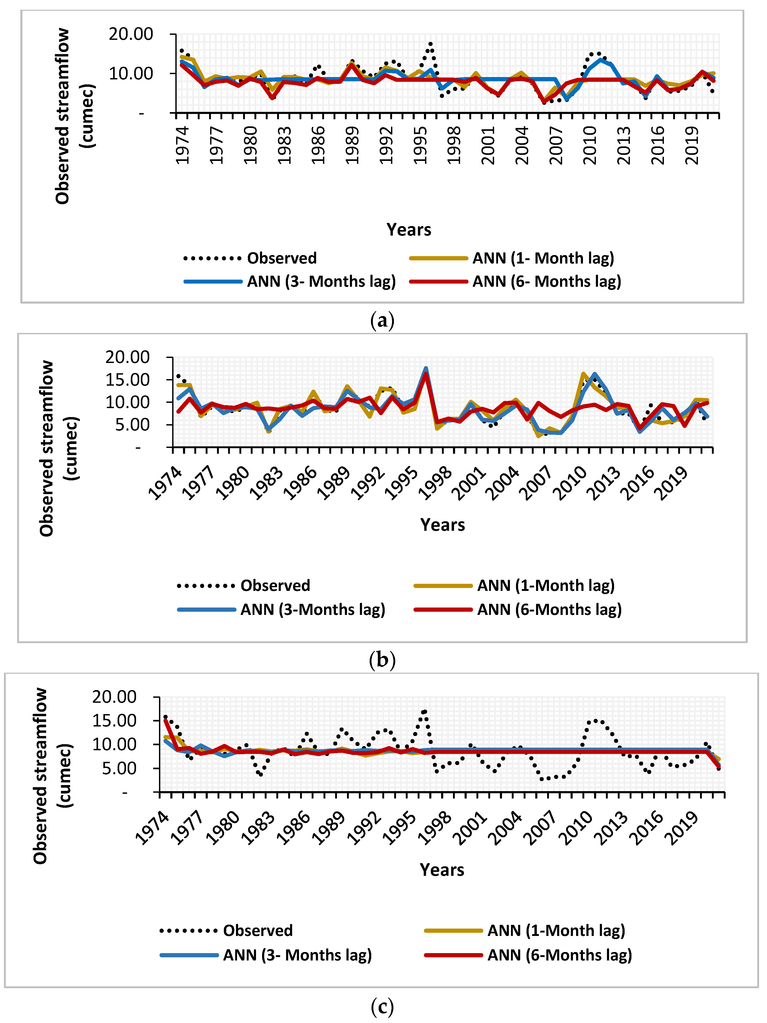
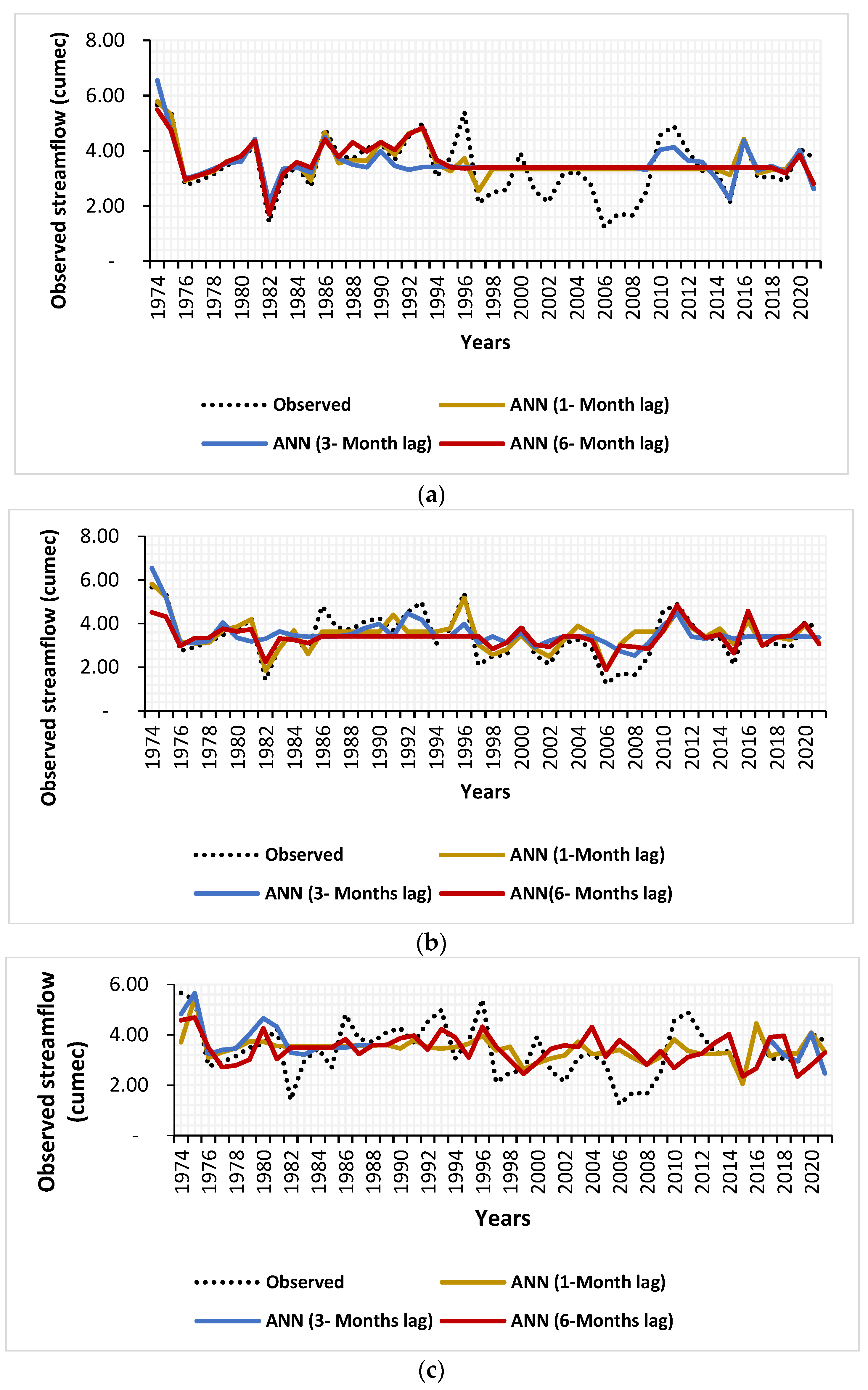
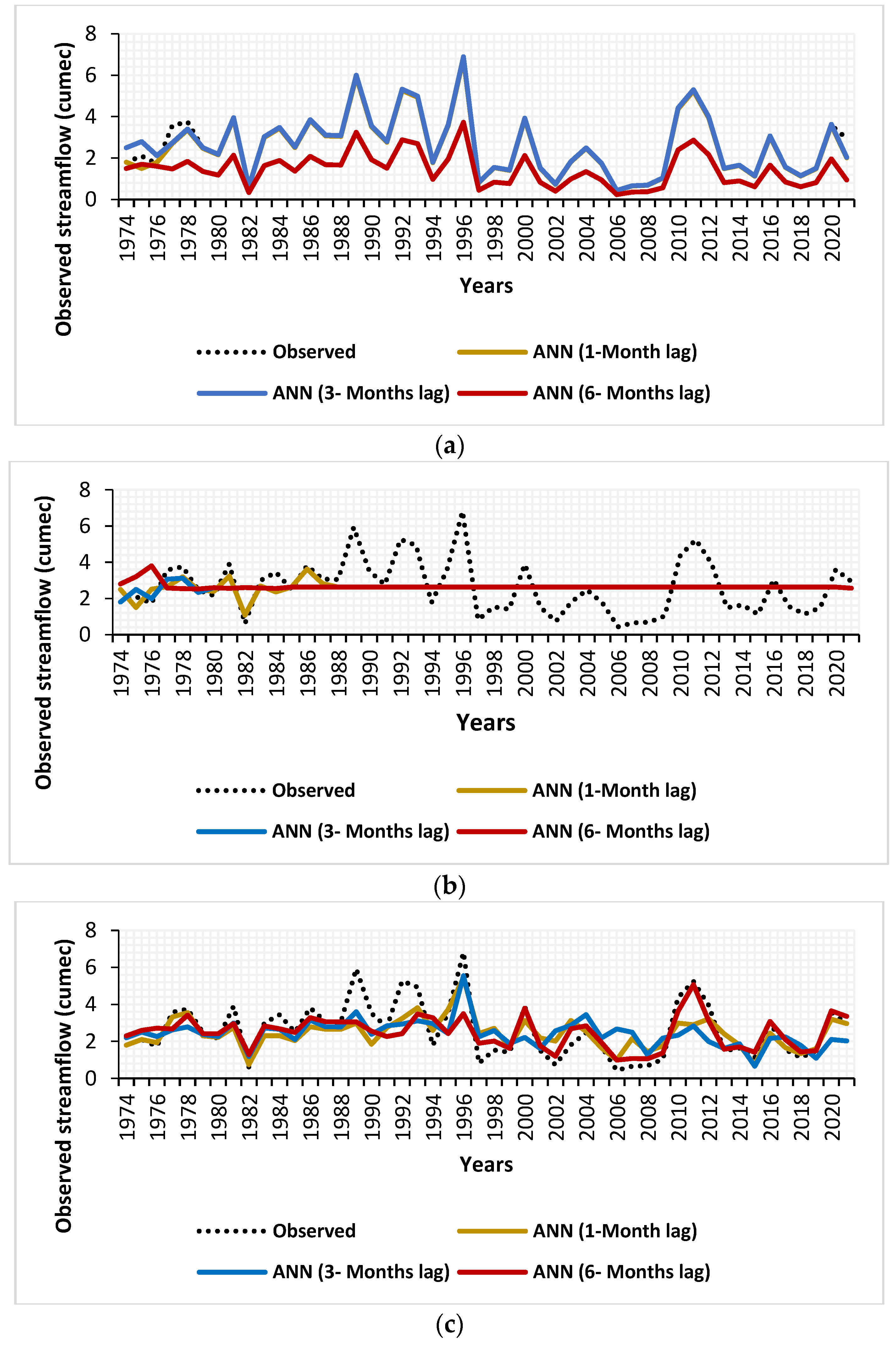
3.3. Time Series Comparison and Discussion

To visualize a deeper comparison of the modeled results, time series plots are also compared, where both the simulated and observed streamflow values are plotted with time. Figure 12, Figure 13 and Figure 14 show the time series comparisons of observed flows and simulated flows using different ENSO indices. From primary observations (as mentioned in the earlier sections), the developed Acheron River model is the best model, with the highest regression correlations as 0.90 and 0.94 using Niño3.4 and Niño4, respectively, and with MSE (0.00 and 0.00) and RMSE (0.00 and 0.00) for one-month lag, as shown in Table 3 and Table 4. The Acheron River models using ENSO also show strong correlations with higher lag months in comparison to other models; however, correlations with 1-month lag is always better than the correlations with 3 or 6-month lag. Figure 12 shows the comparisons of observed and simulated time series values for Acheron River using ENSO indices: Nino3 (Figure 12a), Nino3.4 (Figure 12b) and Nino4 (Figure 12c). From the figures, it is clear that the model using Nino3.4 produced the closest predictions to the observed values with 1-month lag.

Figure 13 show the time series comparisons of observed flows and simulated flows for Rubicon River using different ENSO indices: Nino3 (Figure 13a), Nino3.4 (Figure 13b) and Nino4 (Figure 13c). Again, the model using Nino3.4 produced the closest predictions to the observed values with 1-month lag.

Figure 14 shows the time series comparisons of observed flows and simulated flows for Yea River using different ENSO indices: Nino3 (Figure 14a), Nino3.4 (Figure 14b) and Nino4 (Figure 14c). For Yea River, the model using Nino3 produced the closest predictions to the observed values with 1-month lag. Even simulations with 3-month lagged values produced very close results. Such shifting in the dominance of different indices is likely with the change of geographical location, i.e., the same index is not likely to be dominating the rainfall/streamflow in all the locations.

3.4. Discussions

Developed ANN models perform well in predicting monthly streamflow for three rivers in Victoria, although apparently scatter plots do not look very promising. ENSO-based indices (Nino3, Nino3.4 and Nino4) are found to have good correlations with the monthly streamflows of the studied rivers. The prediction of streamflow one month ahead can be achieved for Acheron River with Nino4 having a correlation value of “0.94”. For the same river, even a prediction six months ahead can be achieved with a correlation coefficient of “0.80”. For Yea River, predictions both one month and six months ahead can be achieved with a correlation coefficient of “0.74”. For both Acheron and Yea Rivers, the highest correlations achieved were with the Nino4, whereas, for Rubicon River, the highest correlations achieved were with Nino3.4. In general, it is known from previous studies that ENSO-based indices have good correlations with the rainfalls of the study region. However, correlations vary with the different ENSO indices. As such, this study reveals particular indices, which are dominant for the selected rivers.

Comparisons of time series graphs reveal that models are capable of simulating continuous monthly streamflow for the selected rivers, especially with a one-month lag period. It is obvious that with the increases in lag months, a model’s capability deteriorates. Usually, such long-term predictions for rainfall are more accurate. However, for streamflow to achieve a higher accuracy is more difficult, as rainfall is a natural phenomenon, which is likely to be related with some natural indices (as selected in this study and many others). Contrastingly, streamflow is a final outcome of rainfall after having several influences by catchment characteristics, which are likely to be altered by human activities. As such, it is more difficult to predict streamflow with the aid of such natural indices. The developed models were capable of capturing most of the peaks and troughs of the time series, although there are some discrepancies, which is acceptable for a complex phenomenon such as streamflow. In this study, the correlations were established only with a single index, whereas some regions might be affected by more than one index. It is likely that consideration of multiple indices for such model generation would help to improve the prediction accuracy, which is recommended to be a future study.

As the significance of other non-ENSO indices (IPO, PDO and IOD) were found to be not very strong, the time series comparisons using these indices were not performed. In Figure 12c and Figure 14b, some of the simulated graphs appeared to be an almost straight line and horizonal. This reveals the insignificance of those indices for the prediction of streamflow in the respective river (i.e., Nino4 for Acheron River and Nino3.4 for Yea River) for the mentioned lagged months.

4. Conclusions

Although seasonal streamflow forecasting has been attempted a lot, continuous streamflow forecasting is rarely practiced. Moreover, all the works on continuous streamflow forecasting were probabilistic estimations. Contrastingly, this paper presents continuous streamflow forecasting with a deterministic approach. To accomplish this, a machine learning ANN technique was used to develop suitable models using dominating climate indices. Previous studies have shown that climate indices have strong effects on streamflow. In this study, the performance of generated models is analyzed based on regression values and different statistical error parameters (MSE, RMSE, MAE and MAPE) for three tributaries of Goulburn River. It is concluded from this study that:

• For all the stations, ENSO-based indices are having significant influence on the streamflow and are able to predict streamflow a few months ahead.
• PDO is found to have the least influence on the streamflow of the selected stations.
• IPO shows moderate (regression values 0.4~0.5) influence on the streamflow of the selected stations; however, this was far below the ENSO-based indices.
• Models for both the Acheron River and Rubicon River show the best performance in predicting streamflow up to 6 months in advance. However, dominating combination of indices are different for Acheron River and Rubicon River.
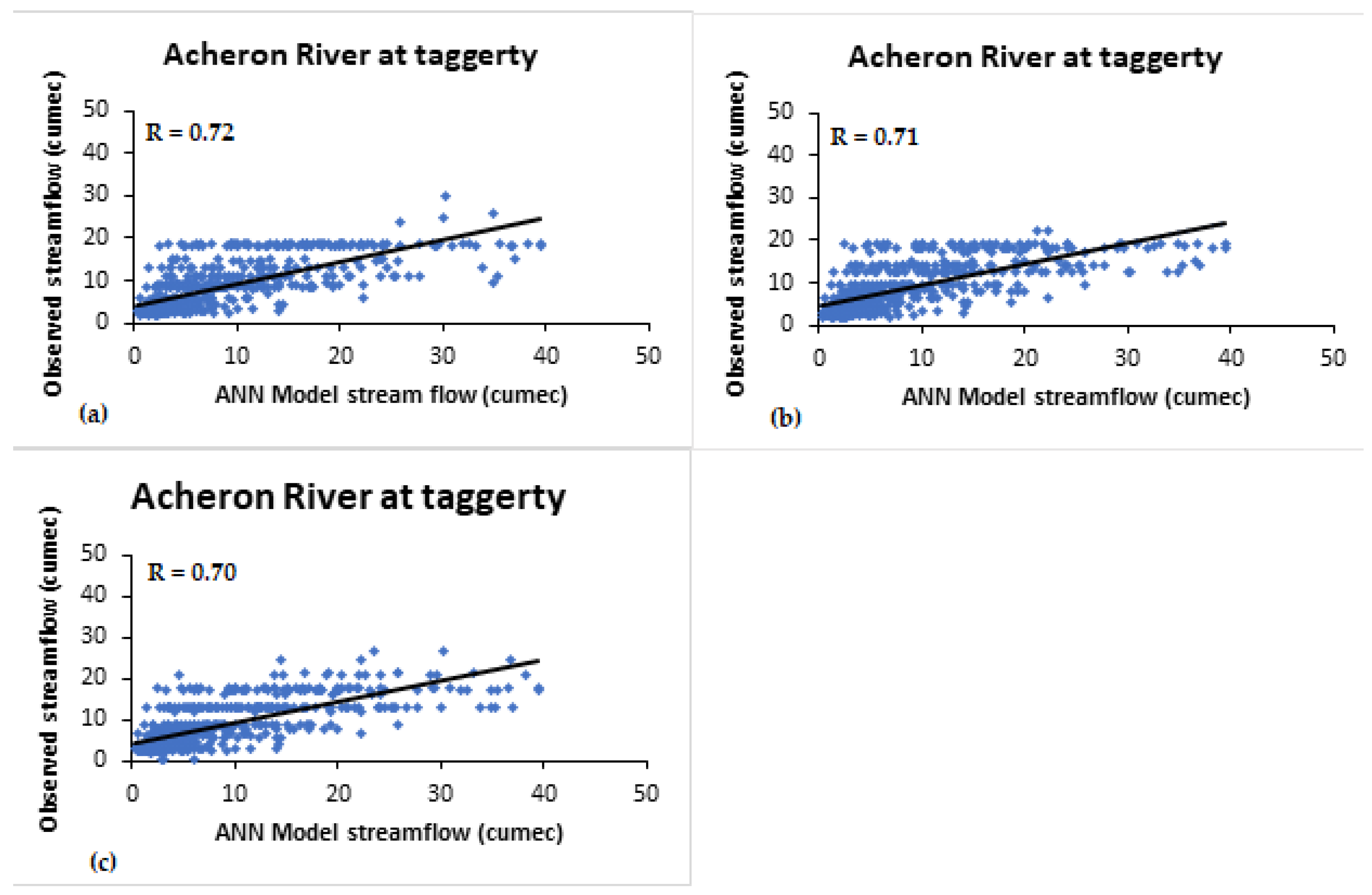
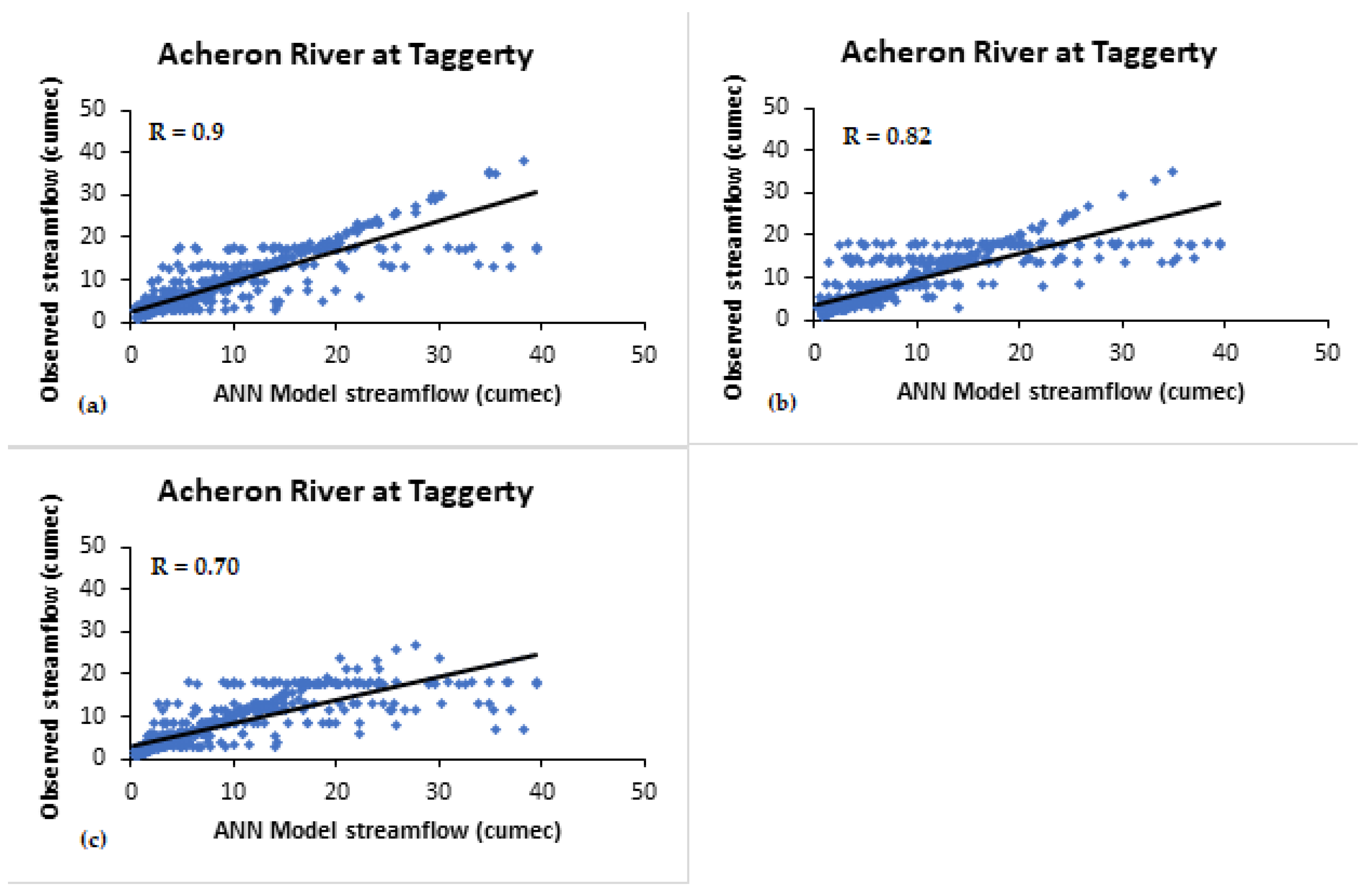
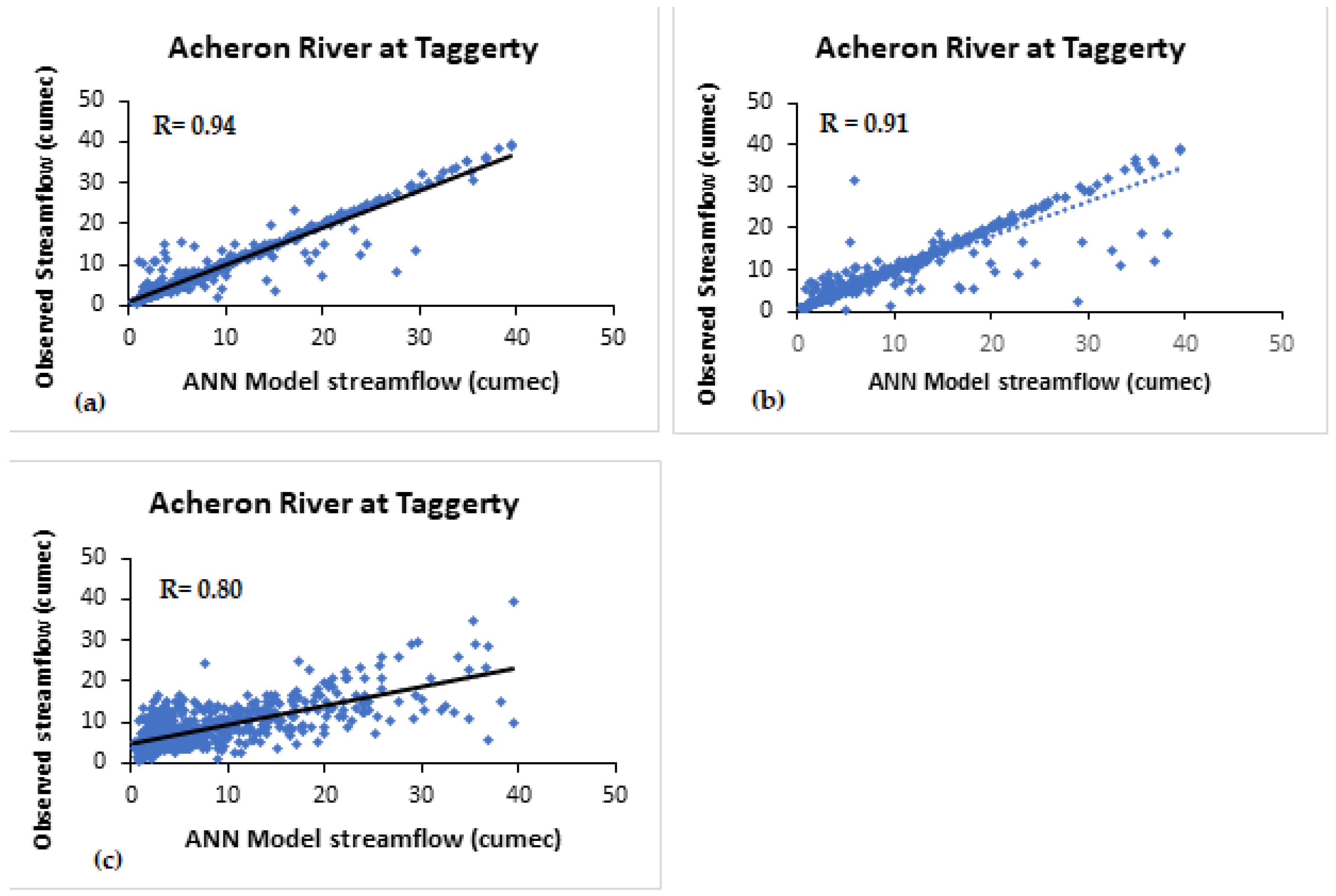
• For Acheron River, Niño3.4 and Niño4 indices were found to be more significant. The correlations between simulated and observed streamflow are 0.90 and 0.94 using Niño3.4 and Niño4, respectively. Corresponding estimation errors are MSE as 0.00 and 0.00, RMSE as 0.00 and 0.00, MAE as 2.03 and 1.06, and MAPE as 37.63 and 17.85, respectively, for one lag month. For 3-month lag, the correlations between predicted and observed streamflow are 0.91 and 0.82 using Niño4 and Niño3.4, respectively.
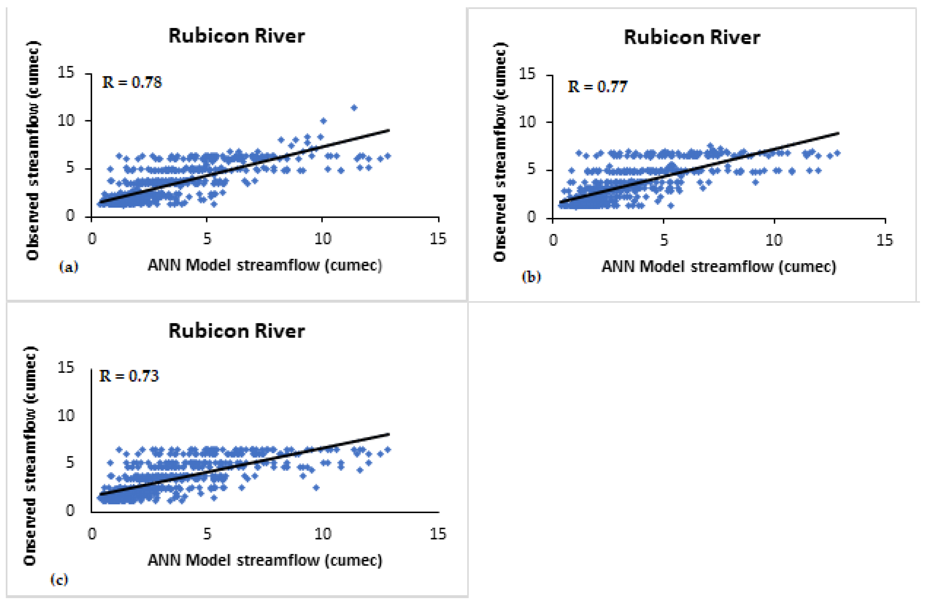
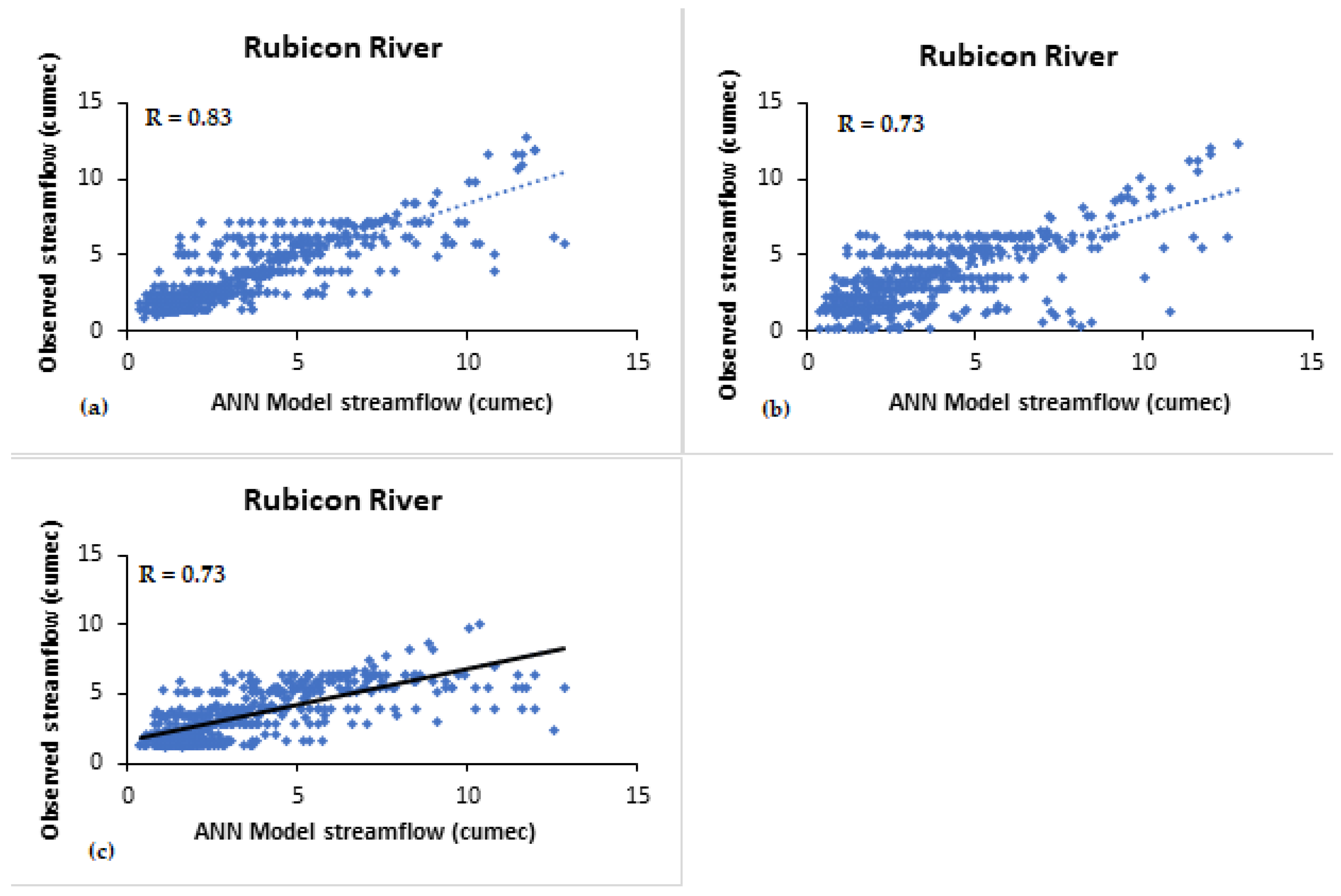
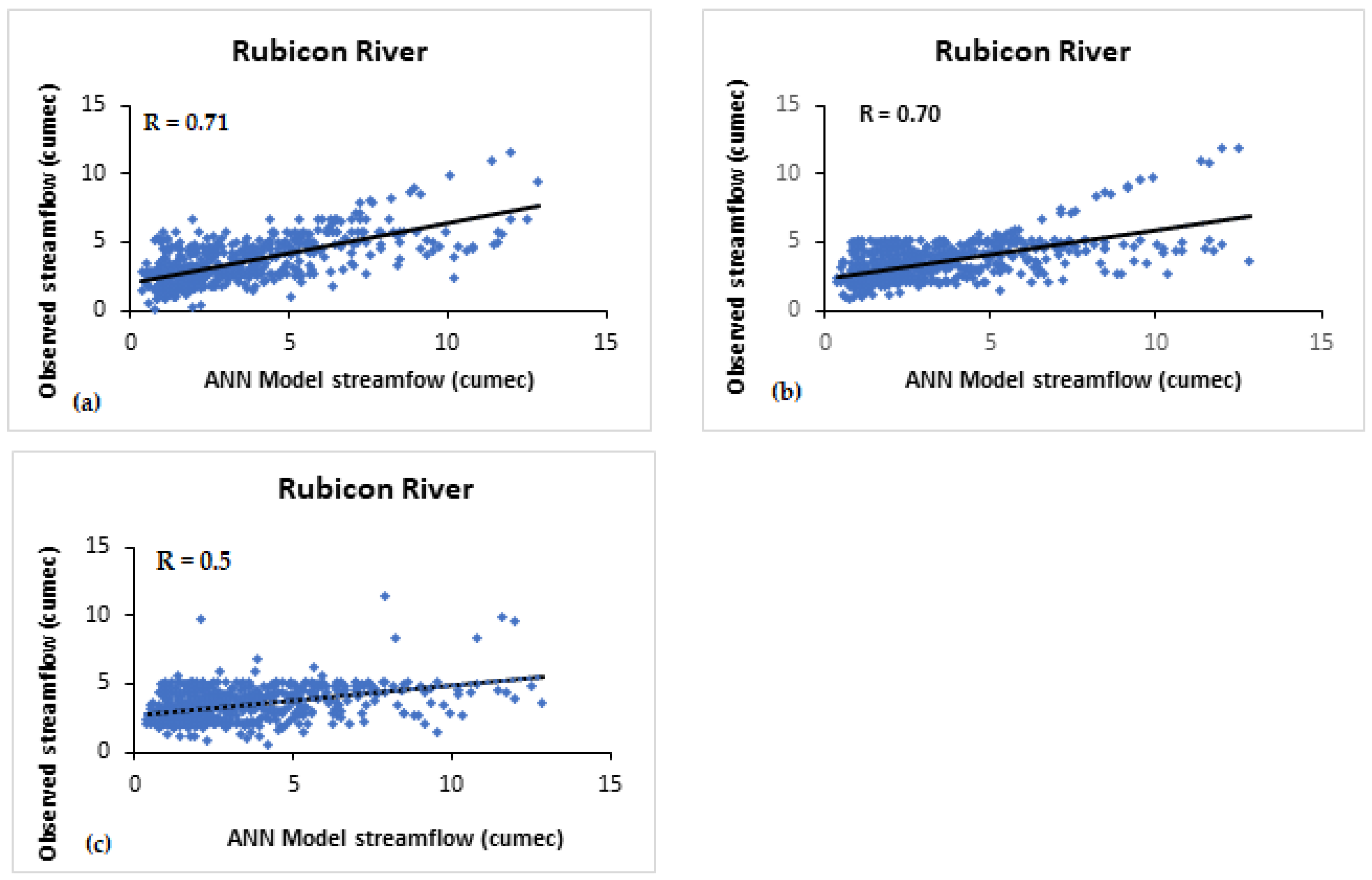
• For Rubicon River, Niño3 and Niño3.4 indices were found to be more significant. The correlations between simulated and observed streamflow are 0.78 and 0.83 using Niño3 and Niño3.4, respectively. Corresponding estimation errors are MSE as 2.4 and 1.91, RMSE as 1.5 and 1.38, MAE as 1.1 and 0.9, and MAPE as 39.76 and 40.67, respectively, for one lag month. For 3-month lag, the correlations between predicted and observed streamflow are 0.77 and 0.73 using Niño3 and Niño3.4, respectively.
• For the predictions 6 months ahead, the Acheron River showed the highest performance, with a regression correlation of 0.8 using Niño3. However, with the Rubicon River model, for 6-month lag a regression correlation of 0.73 was achieved with Niño3 and Niño3.4.
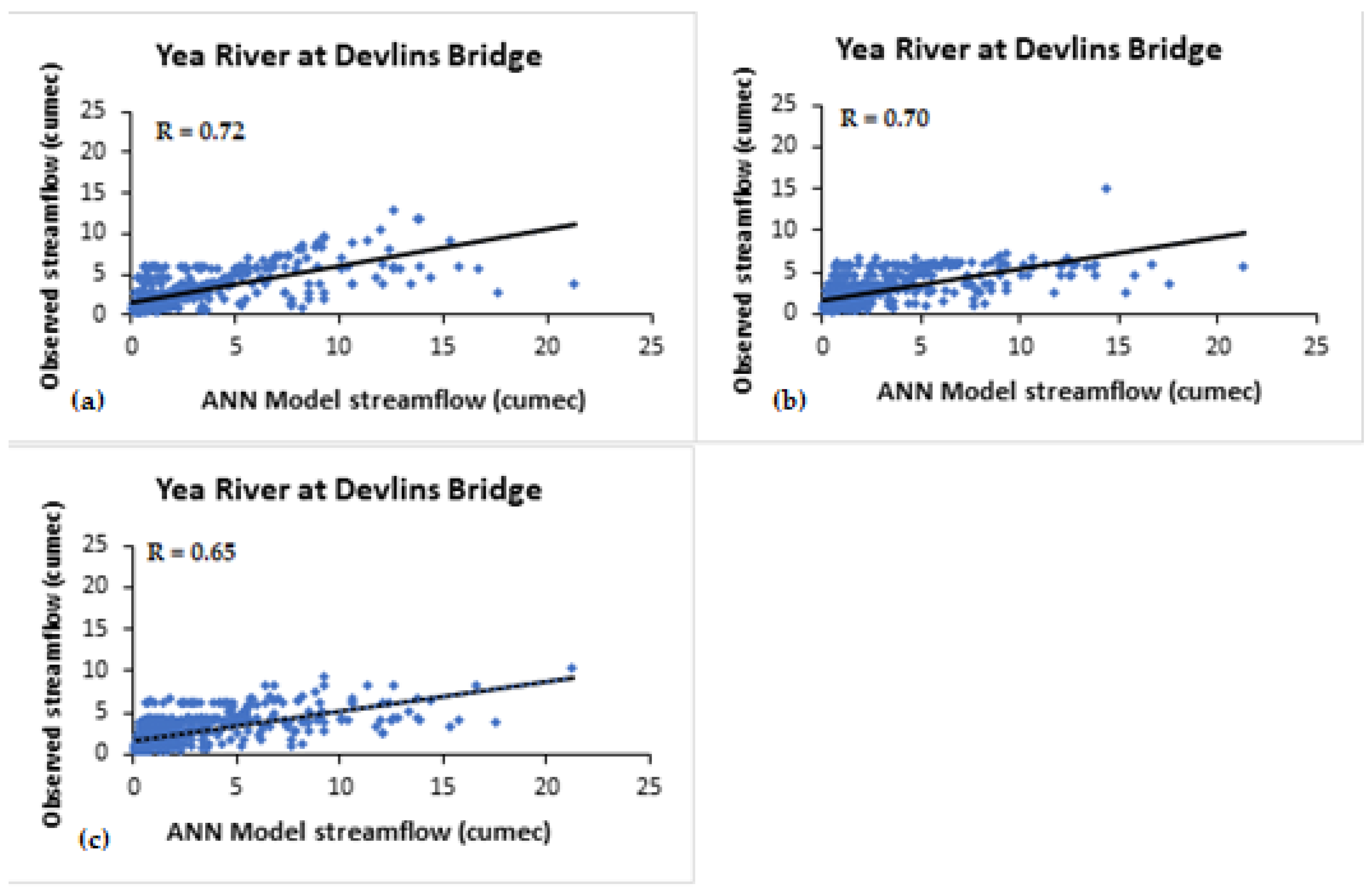
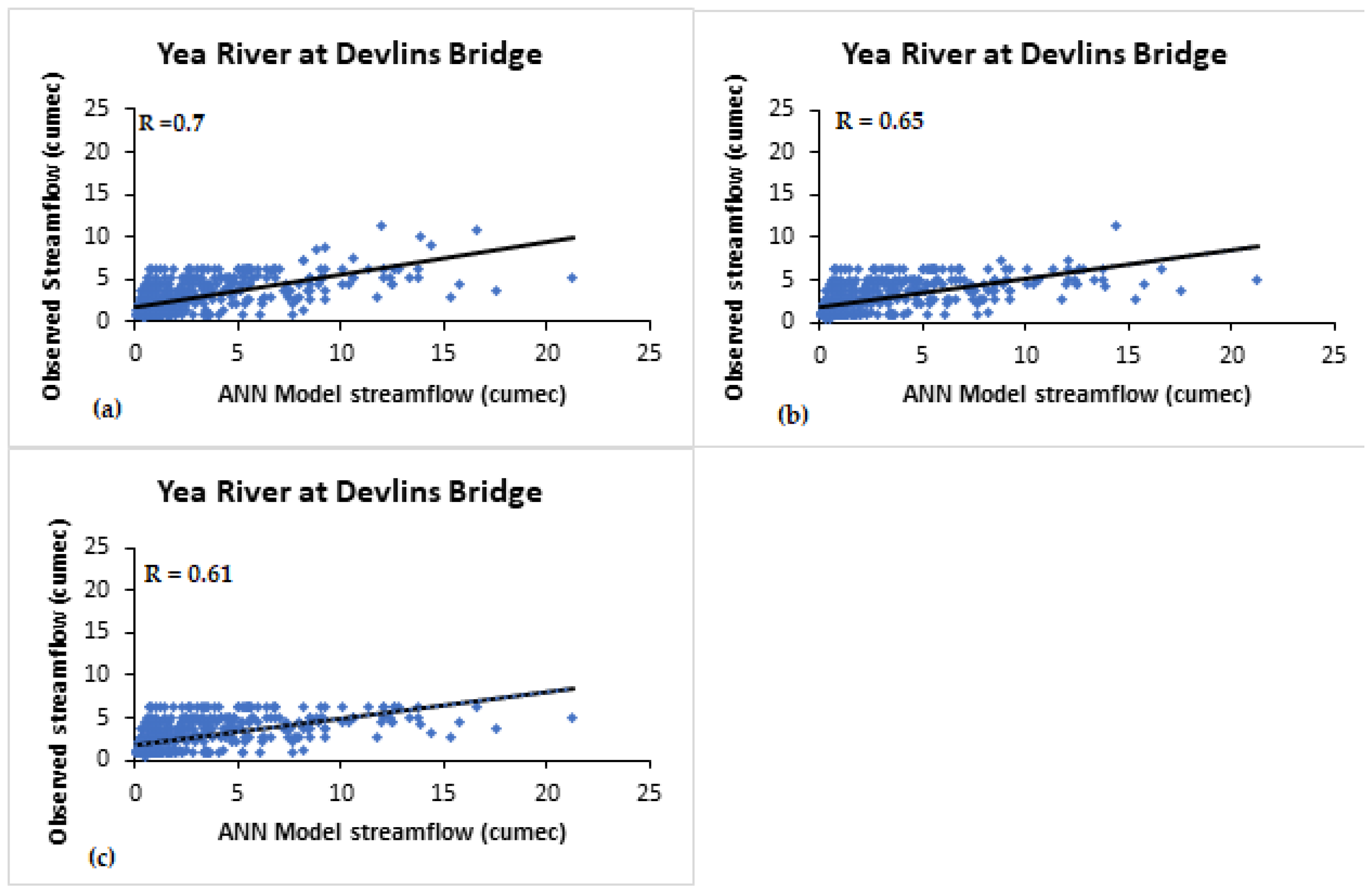
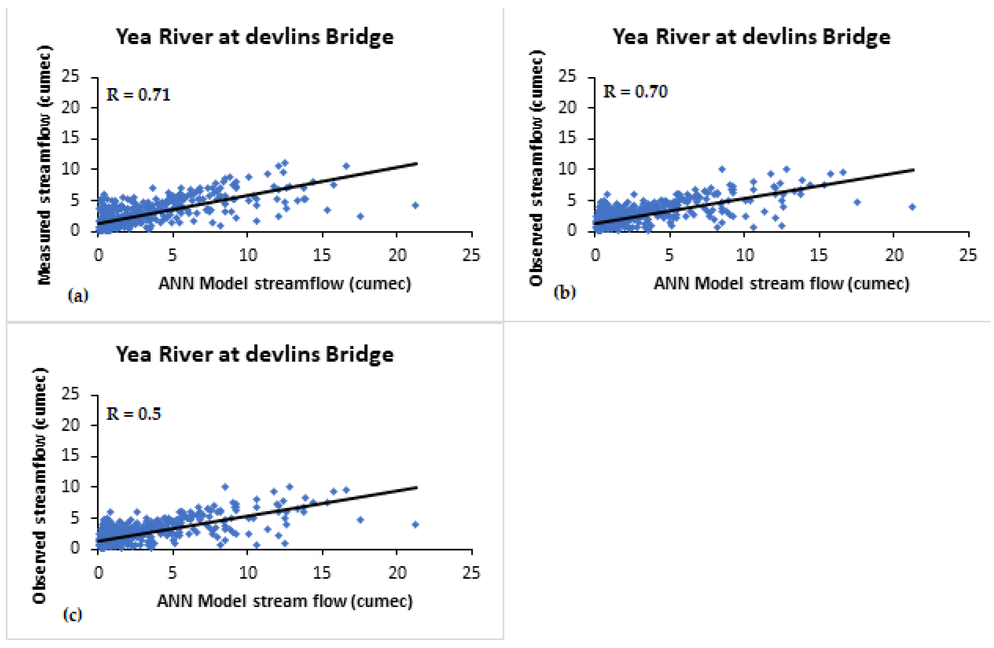
• The regression values for the Yea River models using ENSO indices varied from 0.7 to 0.74 for 1-month lag. For six-month lag, the regression values varied from 0.61 to 0.74. For all the studied cases (for Yea River), the most influencing index was Niño4.
• The time series comparisons for the models with higher correlation values were also found to be good, except that in some cases models were unable to predict the peak values. This is due to the fact that the streamflow is not only dependent on a particular climate index; it is also affected by some other local parameters. In some cases, influences of other local parameters may become superior and discrepancy with the solely index-based models may underperform.
• The performances of the developed models ascertain that such machine-learning-based models using climate indices can be used for other ungauged stations for long-term streamflow forecasting within the region. However, the current study was performed with a single index. It is likely that consideration of a combined effect of multiple indices will provide even better performance. As such, it is recommended that a future study be performed with combined indices, i.e., examining the effect of combined indices on streamflow.

References

1. Akhtar, M.K.; Corzo, G.A.; Van Andel, S.J.; Jonoski, A. River flow forecasting with artificial neural networks using satellite observed precipitation pre-processed with flow length and travel time information: Case study of the Ganges River basin. Hydrol. Earth Syst. Sci. 2009, 13, 1607–1618. [Google Scholar] [CrossRef] [Green Version]
2. Power, S.; Casey, T.; Folland, C.; Colman, A.; Mehta, V. Inter-decadal modulation of the impact of ENSO on Australia. Clim. Dyn. 1999, 15, 319–324. [Google Scholar] [CrossRef]
3. Abbot, J.; Marohasy, J. Using lagged and forecast climate indices with artificial intelligence to predict monthly rainfall in the Brisbane Catchment, Queensland, and Australia. Int. J. Sustain. Dev. Plan. 2015, 10, 29–41. [Google Scholar] [CrossRef]
4. Norel, M.; Katczvnski, M.; Pińskwar, I.; Krawiec, K.; Kundzewicz, Z.W. Climate Variability Indices—A Guided Tour. Geosciences 2011, 11, 128. [Google Scholar] [CrossRef]
5. Duc, H.N.; Rivett, K.; MacSween, K.; Le-Anh, L. Association of climate drivers with rainfall in New South Wales, Australia, using Bayesian model averaging. Theor. Appl. Climatol. 2017, 127, 169–185. [Google Scholar] [CrossRef]
6. Esha, R.I.; Imtiaz, M.A. Assessing the predictability of MLR models for long-term streamflow using lagged climate indices as predictors: A case study of NSW (Australia). Hydrol. Res. 2019, 50, 262–281. [Google Scholar] [CrossRef]
7. Mekanik, F.; Imteaz, M.A.; Gato-Trinidad, S.; Elmahdi, A. Multiple regression and Artificial Neural Network for long-term rainfall forecasting using large scale climate modes. J. Hydrol. 2013, 503, 11–21. [Google Scholar] [CrossRef]
8. Dutta, S.C.; Ritchie, J.W.; Freebairn, D.M.; Abawi, G.Y. Rainfall and streamflow response to El Niño Southern Oscillation: A case study in a semiarid catchment, Australia. Hydrol. Sci. J. 2006, 51, 1006–1020. [Google Scholar] [CrossRef]
9. Ashok, K.; Behera, S.K.; Rao, S.A.; Weng, H.; Yamagata, T. El Niño Modoki and its possible teleconnection. J. Geophys. Res. 2007, 112, C11007. [Google Scholar] [CrossRef]
10. Li, F.F.; Wang, Z.Y.; Qiu, J. Long-term streamflow forecasting using artificial neural network based on preprocessing technique. Sci. Total Environ. 2019, 38, 192–206. [Google Scholar] [CrossRef]
11. Song, X.; Sun, W.; Zhang, Y.; Song, S.; Li, J.; Gao, Y. Using hydrological modelling and data-driven approaches to quantify mining activities impacts on centennial streamflow. J. Hydrol. 2020, 585, 124764. [Google Scholar] [CrossRef]
12. Barsugli, J.J.; Sardeshmukh, P.D. Global atmospheric sensitivity to tropical SST anomalies throughout the Indo-Pacific basin. J. Clim. 2002, 15, 3427–3442. [Google Scholar] [CrossRef]
13. Chattopadhyay, G.S.; Jain, R. Multivariate forecast of winter monsoon rainfall in India using SST anomaly as a predictor: Neurocomputing and statistical approaches. Comptes Rendus Geosci. 2010, 342, 755–765. [Google Scholar] [CrossRef]
14. Hennessy, K.J.; Risbey, J. Trends in rainfall indices for six Australian regions: 1910–2005. Aust. Meteorol. Mag. 2007, 57, 171–173. [Google Scholar]
15. MDBA, Climate and Climate Change. Available online: https://www.mdba.gov.au/importance-murray-darling-basin/environment/climate-change (accessed on 2 May 2021).
16. Water NSW. Available online: https://realtimedata.waternsw.com.au (accessed on 2 August 2022).
17. Jarvis, C.; Darbyshire, R.; Eckard, R.; Goodwin, I.; Barlow, E. Influence of El Niño-Southern Oscillation, and the Indian Ocean Dipole on winegrape maturity in Australia. Agric. For. Meteorol. 2018, 248, 502–510. [Google Scholar] [CrossRef]
18. Chiew, F.H.; Piechota, T.C.; Dracup, J.A.; McMahon, T.A. El Niño/Southern Oscillation and Australian rainfall, streamflow and drought: Links and potential for forecasting. J. Hydrol. 1998, 204, 138–149. [Google Scholar] [CrossRef]
19. Kiem, A.S.; Franks, S.W.; Kuczera, G. Multi-decadal variability of flood risk. Geophhys. Res. Lett. 2003, 30, 1035. [Google Scholar] [CrossRef]
20. Sarle, W.S. Stopped training and other remedies for overfitting. In Proceedings of the 27th Symposium on the Interface of Computing Science and Statistics, Pittsburgh, PA, USA, 21–24 June 1996; pp. 352–360. [Google Scholar]
21. Maier, H.R.; Jain, A.; Dandy, G.C.; Sudheer, K.P. Methods used for the development of neural networks for the prediction of water resource variables in river systems: Current status and future directions. Environ. Model. Softw. 2010, 25, 891–909. [Google Scholar] [CrossRef]
22. Turan, M.E. River flow estimation from upstream flow records by artificial intelligence methods. J. Hydrol. 2009, 369, 71–77. [Google Scholar] [CrossRef]
23. Weather Atlas. Available online: https://www.weather-atlas.com/en/australia/acheron-climate (accessed on 7 August 2021).
24. Nourani, V.; Baghanam, A.H.; Adamowski, J.; Kisi, O. Applications of hybrid wavelet–artificial intelligence models in hydrology: A review. J. Hydrol. 2014, 514, 358–377. [Google Scholar] [CrossRef]
25. Campolo, M. River flood forecasting with a neural network model. Water Resour. Res. 1999, 35, 1191–1197. [Google Scholar] [CrossRef]
26. Humphrey, G.B.; Gibbs, M.S.; Dandy, G.C.; Maier, H.R. A hybrid approach to monthly streamflow forecasting: Integrating hydrological model outputs into a Bayesian artificial neural network. J. Hydrol. 2016, 540, 623–640. [Google Scholar] [CrossRef]
27. Ibrahim, K.S.M.H.; Huang, Y.F.; Ahmed, A.N.; Koo, C.H.; El-Shafie, A. A review of the hybrid artificial intelligence and optimization modelling of hydrological streamflow forecasting. Alex. Eng. J. 2022, 61, 279–303. [Google Scholar] [CrossRef]
28. Kişi, Ö. Streamflow forecasting using different artificial neural network algorithms. J. Hydrol. Eng. 2007, 12, 532–539. [Google Scholar] [CrossRef]
29. DELWP, Department of Environment, Land, Water and Planning. Available online: https://data.water.vic.gov.au/static.htm (accessed on 20 August 2022).
30. Chiang, Y.M.; Chang, L.C.; Chang, F.J. Comparison of static-feedforward and dynamic-feedback neural networks for rainfall–runoff modeling. J. Hydrol. 2004, 290, 297–311. [Google Scholar] [CrossRef]
31. Daliakopoulos, I.N.; Coulibaly, P.; Tsanis, I.K. Groundwater level forecasting using artificial neural networks. J. Hydrol. 2005, 309, 229–240. [Google Scholar] [CrossRef]
32. Abed, M.; Imteaz, M.A.; Ahmed, A.N.; Huang, Y.F. Application of Long Short-Term Memory Neural Network Technique for Predicting Monthly Pan Evaporation. Sci. Rep. 2021, 11, 20742. [Google Scholar] [CrossRef]
33. Abed, M.; Imteaz, M.A.; Ahmed, A.N.; Huang, Y.F. Modelling Monthly Pan Evaporation Utilizing Random Forest and Deep Learning Algorithms. Sci. Rep. 2022, 12, 13132. [Google Scholar] [CrossRef]
34. Ruiz, J.E.; Cordery, I.; Sharma, A. Forecasting streamflows in Australia using the tropical Indo-Pacific thermocline as predictor. J. Hydrol. 2007, 341, 156–164. [Google Scholar] [CrossRef]
35. Kirono, D.G.; Chew, F.H.; Kent, D.M. Identification of best predictors for forecasting seasonal rainfall and runoff in Australia. Hydrol. Process. 2010, 24, 1237–1247. [Google Scholar] [CrossRef]
36. Sang, Y.F. Improved wavelet modeling framework for hydrologic time series forecasting. Water Resour. Manag. 2013, 27, 2807–2821. [Google Scholar] [CrossRef]
37. Chiew, F.H.; McMahon, T.A. El Niño/Southern Oscillation and Australian rainfall and streamflow. J. Water Resour. Res. 2003, 6, 115–129. [Google Scholar]
38. Britannica. “Murray River, Australia”. Available online: https://www.britannica.com/place/Murray-River (accessed on 19 May 2022).
39. Elders Weather. Available online: https://www.eldersweather.com.au/climate-history/vic/yea (accessed on 20 July 2021).
40. Schepen, A.; Wang, Q.J.; Robertson, D. Evidence for using lagged climate indices to forecast Australian seasonal rainfall. J. Clim. 2012, 25, 1230–1246. [Google Scholar] [CrossRef]
41. Taschetto, A.S.; England, M.H. El Niño modoki impacts on Australian rainfall. J. Clim. 2009, 22, 3167–3174. [Google Scholar] [CrossRef] [Green Version]
42. Westra, S.; Sharma, A.; Brown, C.; Lall, U. Multivariate streamflow forecasting using independent component analysis. Water Resour. Res. 2008, 44, W02437. [Google Scholar] [CrossRef] [Green Version]
43. Ghaith, M. Hybrid hydrological data-driven approach for daily streamflow forecasting. J. Hydrol. Eng. 2020, 25, 04019063. [Google Scholar] [CrossRef]
44. Yaseen, Z.M. Prediction of evaporation in arid and semi-arid regions: A comparative study using different machine learning models. Eng. Appl. Comput. Fluid Mech. 2020, 14, 70–89. [Google Scholar] [CrossRef] [Green Version]
45. Robertson, D.E.; Wang, Q.J. A Bayesian joint probability approach to seasonal prediction of streamflows: Predictor selection and skill assessment. In Proceedings of the H2009: 32nd Hydrology and Water Resources Symposium, Newcastle: Adapting to Change, Newcastle, Australia, 30 November–3 December 2009; Engineers Australia: Barton, Australia; pp. 1545–1556.
46. Whiting, J.P.; Lambert, M.F.; Metcalfe, A.V. Modelling persistence in annual Australia point rainfall. Hydrol. Earth Syst. Sci. 2003, 7, 197–211. [Google Scholar] [CrossRef]
47. Yaseen, Z.M.; Jaafar, O.; Deo, R.C.; Kisi, O.; Adamowski, J.; Quilty, J.; El-Shafie, A. Stream-flow forecasting using extreme learning machines: A case study in a semi-arid region in Iraq. J. Hydrol. 2016, 542, 603–614. [Google Scholar] [CrossRef]
48. Sahoo, A.; Samantaray, S.; Ghose, D.K. Stream flow forecasting in Mahanadi River Basin using artificial neural networks. Procedia Comput. Sci. 2019, 157, 168–174. [Google Scholar] [CrossRef]
Figure 1. Map of the Goulburn River catchment including its tributaries.
Climate 11 00152 g001
Figure 2. Flow diagram of research methodology.
Climate 11 00152 g002
Figure 3. Scatter plots of observed and modeled streamflow for Acheron River using Nino3 at different lag months: (a) one lag month; (b) three lag months; (c) six lag months.
Climate 11 00152 g003
Figure 4. Scatter plots of observed and modeled streamflow of Acheron River using Nino3.4 at different lag months: (a) one lag month; (b) three lag months; (c) six lag months.
Climate 11 00152 g004
Figure 5. Scatter plots of observed and modeled streamflow of Acheron River using Nino4 at different lag months: (a) one lag month; (b) three lag months; (c) six lag months.
Climate 11 00152 g005
Figure 6. Scatter plots of observed and modeled streamflow of Rubicon River using Nino3 at different lag months: (a) one lag month; (b) three lag months; (c) six lag months.
Climate 11 00152 g006
Figure 7. Scatter plots of observed and modeled streamflow of Rubicon River using Nino3.4 at different lag months: (a) one lag month; (b) three lag months; (c) six lag months.
Climate 11 00152 g007
Figure 8. Scatter plots of observed and modeled streamflow of Rubicon River using Nino4 at different lag months: (a) one lag month; (b) three lag months; (c) six lag months.
Climate 11 00152 g008
Figure 9. Scatter plots of observed and modeled streamflow of Yea River using Nino3 at different lag months: (a) one lag month; (b) three lag months; (c) six lag months.
Climate 11 00152 g009
Figure 10. Scatter plots of observed and modeled streamflow of Yea River using Nino3.4 at different lag months: (a) one lag month; (b) three lag months; (c) six lag months.
Climate 11 00152 g010
Figure 11. Scatter plots of observed and modeled streamflow of Yea River using Nino4 at different lag months: (a) one lag month; (b) three lag months; (c) six lag months.
Climate 11 00152 g011
Figure 12. Comparison of observed and simulated streamflow time series for Acheron River at 1, 3, and 6-month lag using ENSO indices as an input: (a) Nino3; (b) Nino3.4; (c) Nino4.
Climate 11 00152 g012
Figure 13. Comparison of observed and simulated streamflow time series for Rubicon River at 1,3 and 6-month lag using ENSO indices as an input: (a) Nino3; (b) Nino3.4; (c) Nino4.
Climate 11 00152 g013
Figure 14. Comparison of observed and simulated streamflow for Yea River at 1, 3 and 6-month lag using ENSO indices as an input: (a) Nino3; (b) Nino3.4; (c) Nino4.
Climate 11 00152 g014