
Cascade Structural Sizing Optimization with Large Numbers of Design Variables


1
Department of Civil and Environmental Engineering, University of Cyprus, 75 Kallipoleos Str., P.O. Box 20537, Nicosia 1678, Cyprus
2
Institute of Structural Analysis & Antiseismic Research, National Technical University of Athens, 9, Heroon Polytechniou Str., Zografou Campus, 15780 Athens, Greece
*
Author to whom correspondence should be addressed.
CivilEng 2022, 3(3), 717-733; https://doi.org/10.3390/civileng3030041
Submission received: 6 July 2022
/
Revised: 1 August 2022
/
Accepted: 9 August 2022
/
Published: 13 August 2022
Abstract
:In structural sizing optimization problems, the number of design variables typically used is relatively small. The aim of this work is to facilitate the use of large numbers of design variables in such problems, in order to enrich the set of available design options and offer the potential of achieving lower-cost optimal designs. For this purpose, the concept of cascading is employed, which allows an optimization problem to be tackled in a number of successive autonomous optimization stages. In this context, several design variable configurations are constructed, in order to utilize a different configuration at each cascade sizing optimization stage. Each new cascade stage is coupled with the previous one by initializing the new stage using the finally attained optimum design of the previous one. The first optimization stages of the cascade procedure make use of the coarsest configurations with small numbers of design variables and serve the purpose of basic design space exploration. The last stages exploit finer configurations with larger numbers of design variables and aim at fine-tuning the achieved optimal solution. The effectiveness of this sizing optimization approach is assessed using real-world aerospace and civil engineering design problems. Based on the numerical results reported herein, the proposed cascade optimization approach proves to be an effective tool for handling large numbers of design variables and the corresponding extensive design spaces in the framework of structural sizing optimization applications.
1. Introduction
Structural sizing optimization typically aims at detecting the optimum cross-sectional geometric properties of the structural components that minimize the cost (or material weight/volume) of a structure subject to behavioral constraints (controlling mainly stresses and displacements or drifts) as imposed by design codes. Relevant optimization formulations refer to the weight minimization problem of truss and frame structures [1,2,3,4,5,6,7], the life-cycle cost optimization problem [8], the problem of performance-based structural design optimization [9,10,11], the environmentally driven structural design optimization problem [12,13], etc.
The design variables of a sizing optimization problem are chosen to be parameters defining the cross-sectional shapes and dimensions of structural components. For example, sizing design variables may refer to the cross-sectional type and dimensions of truss and frame members or the thickness of plates and shells. Such design variables are generally discrete, rather than continuous, as fabrication limitations and typical market availability allow cross-sectional shapes and dimensions to be chosen only among very specific options contained in pre-assembled discrete sets.
Structural sizing optimization is formulated in the present work as a single-objective optimization task of the form:
In the above optimization formulation of Equation (1), is the vector of design variables (), which may take values only from a given set D representing the available design options for the cross-sections of the structural components. D is often referred to as the “design space” or “search space” and is defined as a discrete set, in order to enforce only discrete variations of cross-sectional dimensions. denotes the objective function to be minimized (i.e., the structural cost or material weight, volume, etc.). () express the behavioral constraint functions imposed, e.g., by design codes. The objective and constraints of the above optimization problem are generally nonlinear functions of the design variables and need to be evaluated for any candidate optimum design considered by the optimization algorithm.
In sizing optimization, the components of the structure under consideration are usually organized into groups, with all components in a group sharing the same design variable(s). This linking of structural components leads to reduced numbers of design variables and, therefore, to less complicated (more uniform) final structural designs, which are typically preferred in engineering practice. Moreover, the avoidance of large numbers of design variables facilitates the search for the optimum cost solution by the utilized optimizer, since the design space has a more manageable size and is, therefore, more effectively searchable. On the other hand, larger numbers of design variables provide the optimizer with additional design options and can potentially lead to an optimum solution with a better objective function value. This lower-cost final solution is typically associated with significantly increased structural complexity due to less uniformity among the cross-sectional geometries of the components.
Standard optimization schemes, mainly the derivative-free ones (i.e., various metaheuristic algorithms [6]), are most likely to become confused and ineffective when confronted with huge design spaces resulting from large numbers of design variables. In addition, a principal challenge in optimization practice is to optimize a system in the absence of an analytical model describing its behavior. This situation is referred to as “black-box optimization” and is frequently encountered in engineering practice where it is not possible to calculate the derivatives, neither of the objective function, nor of the constraints. In such situations, gradient-based algorithms (i.e., mathematical programming algorithms, etc.) cannot be used, although they might be able to handle problems with large numbers of design variables under certain circumstances [14]. Thus, the optimum cost solution may be hardly detectable within the vast number of design options contained in a huge design space. Consequently, the choice made for the number of design variables in sizing optimization reflects the trade-off between the use of more material and the need for the symmetry and uniformity of structures due not only to practical considerations, but also to computational ones.
Based on the necessity of avoiding the aforementioned computational problems encountered by optimizers when dealing with vast numbers of design options in structural optimization applications, special attention is typically paid to constructing easily manageable (and therefore, relatively small) design spaces. In an effort to relax this necessity, a sizing optimization methodology was presented in [15], which possesses the capability to effectively handle huge numbers of design options resulting from large databases of available cross-sectional types and dimensions.
The present work adopts similar concepts to facilitate the use of large numbers of design variables in structural sizing optimization applications. For this purpose, a series of appropriate Design Variable Configurations (DVCs) is formed for the sizing optimization problem under consideration. First, the initial DVC is defined based on the desired large number of design variables; this corresponds to the finest configuration of design options for the sizing problem at hand. Then, various coarser versions of the initial fine DVC are constructed by merging design variables within the initial DVC; thus, coarser DVCs contain smaller numbers of design variables. Using the assembled series of DVCs, a multi-DVC procedure is applied to explore the design space in the framework of cascade sizing optimization: a number of autonomous optimization stages are performed, which are coupled with the transfer of information between successive stages. Each step of the cascade optimization procedure is performed with a different DVC. Specifically, the initial optimization step starts with the coarsest DVC defined, while subsequent steps use finer and finer DVCs until, finally, the initial (finest) DVC is processed. This multi-DVC cascade computational procedure can be implemented using any optimization algorithm and proves to be very effective in handling large numbers of design variables and corresponding design spaces in the context of sizing optimization problems.
The remainder of this paper is organized as follows. Section 2 generally describes the use of cascading in optimization computations. Section 3 discusses the dilemma of using large or small numbers of design variables in sizing optimization. The proposed multi-DVC cascade optimization procedure is described in Section 4, while numerical results demonstrating the advantages it offers for the case of real-world aerospace and civil engineering problems are presented in Section 5. The paper concludes with some final remarks given in Section 6.
2. Cascade Structural Optimization
Cascade optimization has emerged as a remedy to the fact that there is no unique optimization algorithm capable of effectively handling all existing optimization problems [16]. It has been introduced as a multi-stage procedure, which employs various optimizers in a successive manner to solve an optimization problem [17]. Each autonomous optimization stage of the cascade procedure starts from an initial design , which is either a “cold-start” or a “hot-start”. The cold-start is a user-specified or randomly selected design, which defines the starting solution for the initial optimizer utilized in the first stage of the cascade procedure. The starting solution of the first stage is referred to as a cold-start, because, most often, it lies far from the region of the global optimum. After running the first-stage optimizer, the optimal solution reached is used as the starting solution for the second cascade stage. This new starting solution is called a hot-start, because during the execution of the initial optimizer, the achieved optimal solution is expected to have moved toward the region of the global optimum. Then, each optimization stage of the cascade procedure starts from the optimum solution achieved at the previous stage, i.e., each cascade stage initiates from a hot-start and produces a new hot-start for the next stage. The flowchart of Figure 1 graphically illustrates the cascade optimization procedure.
It is noted that the achieved optimal solution of a cascade stage may first be perturbed using a pseudo-random technique before being adopted as a hot-start for the next cascade stage. When an evolutionary-population-based optimization method is utilized in a cascade stage, its hot-start may be perturbed to produce the remaining members of the initial population. In any case, irrespective of the optimization algorithm employed at each cascade stage, hot-starts provide the coupling of the autonomous optimization computations performed at successive cascade stages.
The actual aim of cascading is to take advantage of the combined strength and the differentiated computations of a number of optimizers executed in a successive manner. This way, we can maximize the exploitation of the optimizers’ advantages and minimize the influence of their disadvantages on the finally attained optimum solution. A trial-and-error process can be followed for any particular optimization case considered, in order to select the optimizer employed at each cascade stage, the exact cascade sequence, the number of cascade stages, the way(s) the differentiation of the computations among cascade stages is achieved, etc.
Although the basic concept of cascading assumes the utilization of a different optimization algorithm at each cascade stage, the case of invoking the same optimizer at more than one (or even at all) cascade stages should not be excluded. A number of cascading variations have been successfully implemented in structural optimization applications: various gradient-based optimizers were utilized at the cascade stages in [17,18,19,20]; a gradient-based optimizer and a response surface approach were integrated in the framework of a cascade procedure in [21]; the same evolutionary optimizer was employed at all cascade stages in [15,22]; both gradient-based and evolutionary optimizers were applied one after the other in [23]; cascading was implemented also in a general-purpose design optimization platform [24] and applied to real-world structural design optimization problems [12].
In the cascade structural optimization procedure implemented in the present work, all cascade optimization stages are performed with the same derivative-free optimizer in a way similar to that followed in [15]. Specifically, in the first numerical example of Section 5, all cascade stages are executed using a discrete evolution strategies algorithm; in the second numerical example, the cascade stages are executed using a discrete simulated annealing algorithm. The differentiation of the search paths followed by these optimizers during the cascade stages is ensured by changing the initial conditions of individual optimization runs. For this purpose, we used at each cascade stage:
- A different initial solution vector (each cascade stage initiates from its corresponding hot-start except from the initial stage, which initiates from a random cold-start);
- A different seed for the random number generator of the non-deterministic optimization process;
- A different design variable configuration (as described in Section 4).
It may happen that a particular cascade stage initiates from the same hot-start as the previous stage. This is possible when the previous stage does not achieve any improvement in the objective function value and yields its hot-start as the best attained solution. If the two cascade stages employ also the same design variable configuration, the differentiation of the search paths is still guaranteed through the different initial seeds used for the random number generator. Differentiated search paths can also be obtained by utilizing a different database of cross-sectional geometries at each cascade stage [15]. The cascade procedure may be continued until no improvement in terms of the objective function value is observed after a user-defined number of optimization stages.
It should be finally mentioned that cascading induces the need for performing large numbers of structural analyses during the successive optimization runs and is consequently associated with high overall computing costs. Such demanding computations can be executed in affordable processing times by drastically accelerating the optimization runs of the cascade stages with the use of parallel processing, advanced solution techniques, and metamodel-assisted predictions (e.g., using neural networks) [23,25].
3. The Dilemma of Using Large or Small Numbers of Design Variables
A detailed formulation of a structural sizing optimization problem would contain a large number of design variables controlling all design decisions for the structural system considered. Thus, assuming, e.g., a truss or frame structure, the design variables introduced could correspond to the cross-sectional properties of each truss/frame member, i.e., separate design decisions for each member’s cross-section would be allowed. Thus, the optimizer invoked to process such a sizing problem is given the possibility to really optimize the objective function (i.e., to minimize the total cost of material required for all structural components) by detecting the optimum solution within the vast amount of all possible design options.
However, a large number of design variables does not only offer advantages to the optimizer, it also introduces difficulties. Since the resulting design space becomes extensive, its exploration is not a trivial task for any optimization algorithm. The huge number of available design options typically confuses an optimizer, especially a non-deterministic one, and radically decreases the potential of searching effectively for a high-quality solution. As a result, the optimizer is most likely to become trapped in a purposeless search, which is like shooting in the dark to hit a target. Such a process can deliver a final result of acceptable quality only by chance. It may be so ineffective that it is unable even to roughly locate the areas of appropriate design variable values. Thus, although, theoretically, the large number of design variables may be advantageous for the structural optimization process, its exploitability in practice is seriously questioned.
Another issue to consider is the complexity/non-uniformity introduced in the final design when large numbers of design variables are utilized. A final design consisting of many non-identical structural components is relatively complicated. As a result, a number of disadvantages arise:
- An increase in construction/manufacturing cost should be expected, because a complicated design is more difficult to implement and supervise compared to a simple design consisting of many identical components.
- Manufacturing or ordering many non-identical components is most likely to be associated with additional cost compared to the same material weight/volume distributed over fewer types of components.
- A complicated design is further exposed to human error, especially during the construction/manufacturing phase.
Thus, assuming that the global optimum can be actually identified (or at least approached) when a large number of design variables is used, it has to be decided whether the reduction in material weight/volume achieved compared to a smaller number of design variables compensates the disadvantage of increased complexity introduced in the final design.
The achievable material weight/volume and the design complexity function as conflicting criteria within a multi-criteria decision-making setting. The trade-off relation between these two criteria can be theoretically described by a type of “Pareto front” curve, which is conceptually illustrated in Figure 2. The points below the curve correspond to infeasible designs. The points above the curve correspond to either infeasible or non-optimal feasible designs. The points on the curve correspond to feasible optimal designs. Hence, the trade-off curve of Figure 2 includes all possible “non-dominated” combinations of numbers of design variables and corresponding best attainable objective function values. Any of these combinations is “non-dominated” in the sense that there is no other combination having both a smaller number of design variables and a lower attainable objective function value. Thus, for any two points on the curve, one corresponds to a heavier and simpler design, while the other corresponds to a lighter and more complicated design (Figure 2).
Few applications of structural optimization using large numbers of design variables are reported in the literature. For example, structural optimization problems with up to 200 design variables were solved in [1,2,6,13]. Typically, the number of design variables employed in structural optimization applications is much smaller. In order to avoid large numbers of design variables, the components of the structure considered are usually organized into groups, with all components in a group sharing the same design variable(s) (e.g., [7,9,11,13,15]). This way, the resulting design space is more manageable and, therefore, more effectively searchable. The grouping of members in order to introduce shared design variables is based on the engineer’s experience and intuition and may involve a limited number of test structural analyses. This “manual” process obviously demands human effort and costs time before even invoking the optimizer. A poor grouping may misguide the optimizer and lead to suboptimal or even low-quality final designs.
Since richer design options are offered by a more extensive search space, it is generally expected that the globally optimum structural design obtained with a large number of design variables will correspond to a lower objective function value compared to that yielded by the global optimum based on a smaller number of design variables. Nevertheless, in a practical application tackled with a standard optimizer, the global optimum is hardly detectable and is most likely to remain “hidden” within a huge design space. Therefore, a higher-quality optimization result could be anticipated with a rationally assembled configuration employing not so many design variables.
4. Cascade Sizing Optimization Using a Series of Design Variable Configurations
In this work, the concept of cascading is adapted to the particular need of effectively handling structural sizing optimization problems with large numbers of design variables. More specifically, a cascade sizing optimization approach is proposed, which employs a series of configurations (DVCs) for the design variables of the problem at hand. Each stage of the cascade optimization procedure is performed with a different DVC. The initial DVC includes all design variables that can be defined for the sizing problem considered. Hence, is the finest possible configuration of design options for the particular problem and includes the largest possible number of design variables . Then, n coarser versions , , …, of are produced by merging the design variables of . Typically, each design variable in a coarser DVC is shared by more structural components than in a finer DVC; therefore, the coarser DVC contains a smaller number of design variables than the finer DVC. Thus, a set S of DVCs is assembled:
with:
where , , …, are the number of design variables for configurations , , …, , respectively. The set S contains DVCs, with being the coarsest configuration and the finest one.
The assembled set S of DVCs can be used to execute a multi-DVC cascade sizing optimization procedure, in order to effectively explore the large design space associated with the fine configuration . A general flowchart of this procedure is presented in Figure 3. In order to facilitate the description of the procedure, without loss of generality, let us set and , i.e., two coarser DVCs of the fine configuration are constructed for a particular sizing optimization problem. The first optimization stage of the cascade procedure uses the coarsest DVC available in S () and initiates from a cold-start , which is a vector with randomly generated values for the design variables of . In this initial stage, the implemented optimizer has to deal with the relatively small number of design variables of the coarse configuration , which produces a manageable design space and generally allows for a smooth and non-problematic optimization run. Next, the optimum solution vector finally attained from the first cascade optimization stage needs to be converted to a vector with values for the design variables of the finer configuration . For this purpose, information on the design variable number(s) of each member in configurations and is exploited. After this conversion, the obtained vector is adopted as the hot-start to initiate a new cascade optimization stage using configuration . The optimum solution vector finally attained from the second cascade stage is converted to a vector of size , which is set as the hot-start for performing the final cascade optimization stage using the finest configuration . The optimum solution vector finally attained at the third cascade stage is the optimum solution achieved by the overall multi-DVC cascade sizing optimization procedure. Note that the subscript d denotes the current cascade stage (except for subscript “0”, which denotes an initial solution vector for an optimization run). Thus, configuration is processed at cascade optimization stage , which produces the optimum design (Figure 3).
The multi-DVC cascade sizing optimization procedure is applied by executing cascade optimization stages, in order to process all available DVCs one by one. The first cascade stage initiates from a random cold-start and attains an optimum design, which is passed to the second cascade stage, in order to initialize a new optimization run carried out using a DVC with a larger number of design variables. Several cascade optimization stages can be performed in the same manner with subsequent steps using finer and finer DVCs. The cascade process is continued until all constructed DVCs are utilized, i.e., until, finally, the DVC with the largest number of design variables () is processed. To ensure more effective design space exploration, more than one cascade stage can be carried out using a single DVC (by modifying the employed optimizer and/or the initial seed for the utilized random number generator, the same DVC can be employed in a number of successive cascade stages before proceeding to a finer DVC). Whether the utilized DVC changes between two successive cascade stages or remains the same, the coupling between these stages is realized by initializing the new stage using the finally attained optimum design of the previous stage.
The first stages of the cascade procedure executed with the coarsest DVCs aim at a basic non-detailed search of the full design space. This search is facilitated by the manageable DVCs handled, which avoid confusing the employed optimizer with huge design spaces. Thus, the areas of appropriate design variable values are identified by detecting (near-)optimum solutions among the relatively limited design options provided. As the numbers of design variables processed in the cascade stages become larger, a more detailed representation of the full design space is offered and the optimizer is given the opportunity to improve the quality of the optimal solution reached. The gradual upgrade of the optimal design vector over a number of cascade stages is practically feasible due to the transfer of the optimization results between successive stages, in order to exploit in each new optimization stage the search space exploration efforts performed up to the previous stage. Thus, despite the large design spaces handled, the appropriate initialization of each cascade stage prevents the optimizer from being trapped in a process of purposeless and ineffective searching. In the final cascade stages utilizing the finest DVCs, relatively small adjustments to an already good-quality design occur, in an effort to identify (or at least approach) the globally optimum design. Hence, the first optimization stages of the cascade procedure serve the purpose of basic design space exploration, while the last stages aim at fine-tuning the achieved optimal solution.
5. Optimization Results
The effectiveness of the proposed multi-DVC cascade sizing optimization approach was assessed using two real-world design problems from the fields of aerospace engineering (wing box design) and civil engineering (building design).
5.1. Test Problem 1: Wing Box
The first test problem considered to evaluate the cascade optimization approach for large numbers of design variables proposed in this work was a wing box sizing optimization problem. The particular wing box optimized was the primary structure of an Airbus A320 wing. It contains the key structural components of the wing (spars, ribs, braces, bars, struts, etc.) and is enclosed by the upper and lower skins of the wing. Wing box optimization was studied in a number of publications (e.g., [26,27,28,29]).
In order to simulate the structural response of the wing box, a three-dimensional Finite Element (FE) model was developed in Abaqus/CAE [30], which is composed by 9050 elements and 40,674 degrees of freedom. A view of the generated FE mesh is given in Figure 4. The external upper, lower, and side surfaces of the wing box, as well as the enclosed rib surfaces were modeled using triangular and quadrilateral shell elements. The openings of an elliptical shape providing working access were placed at the lower box surface and at the smallest rib lying at the free edge of the box (Figure 4). Stiffeners installed longitudinally and at certain angles to the box were modeled using bar elements. All structural components comprising the wing box were made of aluminum alloy. The connection of the wing to the main body of the aircraft was modeled by assuming clamped support for the wing. Specifically, all degrees of freedom of the nodes lying at the perimeter of the largest rib and being in contact with the aircraft’s main body were fully constrained. The external surface loads imposed on the wing were modeled as concentrated loads acting on the perimeter nodes of the ribs.
In the sizing optimization problem considered in this part of the study, the aim was to minimize the total material volume of the upper, lower, rib, and side surfaces of the wing box by determining appropriate thicknesses for these surfaces. Thus, sizing design variables were defined, which control the aforementioned thicknesses. Two types of constraints were imposed to appropriately limit: (a) the maximum von Mises stress developed in the structural model and (b) the maximum vertical deflection arising at the free edge of the wing. A discrete Evolution Strategies (ES) algorithm was employed to solve this optimization problem. In particular, the (10,10)ES scheme was applied (10 parent and 10 offspring vectors were used) as described in [31], where more details on this evolutionary algorithm are also provided. Any optimization run, whether it is an individual (non-cascade) run or a run of a cascade stage, was stopped when no improvement in the best attained objective function value was observed for four consecutive ES generations.
In the framework of the optimization procedure, any candidate optimum solution was assessed by invoking Abaqus/CAE to conduct an FE analysis for the surface thicknesses defined by the particular solution processed. The optimization program and Abaqus/CAE were linked through specially developed interface software, which automatically passes data and results from the optimization algorithm to Abaqus/CAE and vice versa. The simple, yet effective multiple linear segment penalty function [24] was used in this study for handling the constraints. According to this technique, if no violation was detected, then no penalty was imposed on the objective function. If any of the constraints were violated, a penalty, relative to the maximum degree of the constraints’ violation, was applied to the objective function.
Table 1 provides information about the five DVCs defined for this sizing optimization problem. Hence, and , i.e., four coarser DVCs of the fine configuration were constructed. The total number of design variables in the five DVCs ranged from 4 to 108. As an illustrative example, Figure 5 indicates how the design variables were allocated to the wing box surfaces for configuration ( design variables in total). Each design variable corresponds to the thickness of a group of shell elements. Thicknesses were allowed to take only specific pre-defined values; therefore, all design variables were discrete. Finer DVCs gave the optimizer the opportunity to select designs with larger thickness variations in the wing surfaces, which might result in substantial cost savings due to the more effective use of material.
Figure 6 reports the ES optimization results obtained for the wing box problem. The convergence histories presented for non-cascade optimization runs clearly show the inability of the optimizer to effectively search the design space available in each optimization case. The optimizer converges to suboptimal solutions, which tend to be of lower quality as the number of variables is increased, and the resulting design space becomes larger. The best solution from non-cascade runs was attained using the coarsest DVC available in set S (), which has only four design variables and produces an easily searchable design space of a small size. It is also interesting to notice the long non-cascade run using the finest DVC available in S (), in which the objective function value was improved at a rather slow rate and converged to a very high value. This reveals the difficulty encountered by the optimizer in handling the large number of design variables defined for ().
On the other hand, the proposed multi-DVC cascade optimization procedure performed consistently despite being confronted with large numbers of design variables. Overall, cascade stages were executed, in order to process all DVCs in S one after the other, as described in the flowchart of Figure 3. The non-cascade run using was adopted as the first cascade stage. This provides the hot-start for the second cascade stage, in which is used. As can be seen in Figure 6, the cascade procedure manages to deliver lighter designs for finer DVCs and, finally, achieves a much lower objective function value than any non-cascade optimization run. Specifically, the best wing box design achieved with the cascade procedure was about 50% lighter than the best design obtained without cascading (using ) and 70% lighter than the design attained without cascading using .
An interesting by-product of the optimization runs conducted is the trade-off information depicted in Figure 7, which provides the results of Figure 6 in the form of Figure 2. Figure 7 reveals again the poor performance of non-cascade optimization runs for fine DVCs. Actually, the solution attained using “dominates” all solutions obtained with the other (finer) DVCs. On the contrary, “non-dominated” optimum solutions are achieved with the multi-DVC cascade optimization procedure. In fact, the solution attained using cannot be improved upon using , which means that the solution attained using dominates the solution obtained using . Thus, there is no reason to adopt (), because it does not lead to a lower objective function value than (). Moreover, () leads to practically the same objective function value as (). Thus, the final decision should actually be between 4 (), 20 () and 80 () design variables. It has to be decided whether the reduction in material volume gained with a larger number of design variables compensates the disadvantage of the additional complexity of the final design.
Inevitably, the gains in material quantity using finer DVCs with the cascade optimization approach were obtained at some additional computational cost. Figure 8 demonstrates the relative performance of the non-cascade (single-DVC) and cascade (multi-DVC) optimization approaches. It can be seen that the non-cascade optimization runs using , , , and require about half (or even less) of the computational cost compared to the overall multi-DVC cascade procedure, but yield rather poor final designs. The non-cascade optimization run using exhibits comparable computational demands as the overall cascade procedure, but is not able to attain a satisfactory objective function value. Thus, the multi-DVC cascade optimization approach is indeed computationally more expensive, but performs computations that are really useful in making an effective search and directing it toward a high-quality solution. Such effectiveness is not shown by standard non-cascade optimization runs using fine DVCs, as the computations seem to be wasted in conducting poorly guided and, therefore, unproductive searches.
5.2. Test Problem 2: 36-Story Steel Space Frame
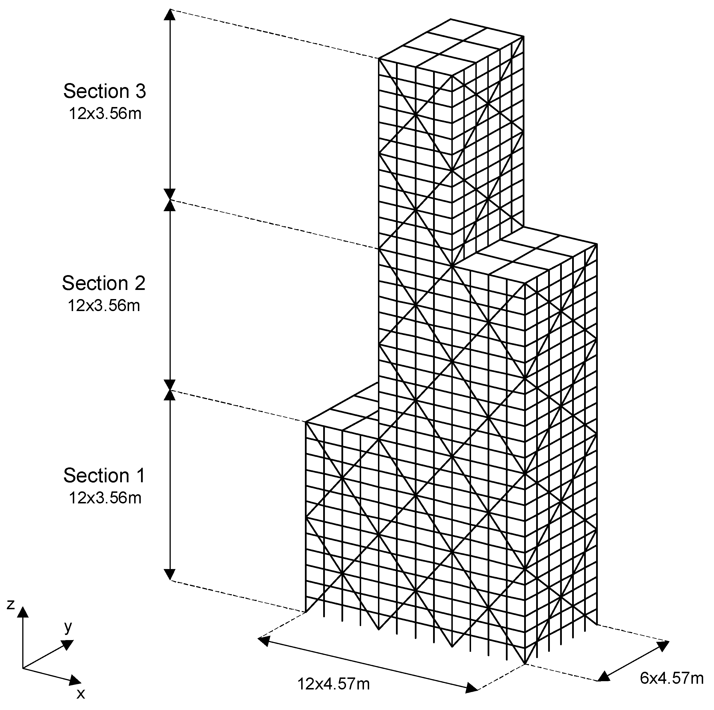
The second test problem examined in this study is the 36-story steel building of Figure 9, which was modeled as a space frame with 3228 elements and 7992 degrees of freedom. The space frame was clamped to the ground and was subjected to vertical dead and live loads and horizontal wind loads. It was divided in the vertical direction into three 12-story sections, as shown in Figure 9. The frame has steel columns and beams with I-shaped cross-sections and steel cross-bracings with L-shaped cross-sections. This test problem was previously investigated in [15], while a similar structure was considered in [8].
In this sizing optimization problem, the aim is to minimize the total material weight of the structure. The constraints imposed involve member stresses checked with respect to the design provisions of Eurocode 3 [32], as well as inter-story drifts, which are limited below the threshold value , where h is the story height. The sizing design variables defined control the cross-sectional geometries of the frame’s steel members.
In order to produce suitable member groups for the sizing optimization procedure, the following member types of the space frame were distinguished:
- Four types of columns: corner columns, outer columns, inner columns in unbraced frames, and inner columns in braced frames;
- Three types of beams for the two lower sections 1 and 2: outer beams, inner beams in unbraced frames, and inner beams in braced frames;
- Two types of beams for the upper section 3: outer and inner beams;
- Two groups of bracings in the longitudinal and transverse directions.
Based on these member types, three DVCs are defined in Table 2, i.e., and . Each design variable corresponds to the cross-section of a member group. The three DVCs result from the different groupings of members within each of the structure’s sections 1, 2, and 3. For example, in configuration , the columns of section 1 are grouped every two stories, which means that section 1 is divided in the vertical direction into six sub-sections; since there are four types of columns, the total number of column groups (and corresponding design variables) in section 1 is . The total number of design variables in the three DVCs defined ranges from 25 to 186. The options for the design variables of the structure’s columns and beams are contained in a large database with 200 standard I-shaped cross-sections. The options for the design variables corresponding to the cross-bracings are contained in a smaller database with 15 standard L-shaped cross-sections. Since specific pre-defined cross-sectional geometries are included in these databases, all sizing design variables utilized are discrete.
Figure 10 depicts the results obtained by applying the proposed multi-DVC cascade optimization procedure. The convergence history and the finally attained optimum solution for the first cascade optimization stage using were taken from [15]. Hence, the first cascade stage was performed with a multi-database optimization procedure using a discrete ES algorithm. More specifically, in order to effectively deal with the large database of I-shaped cross-sections, which contains 200 items, coarse versions of it with fewer items were formed (the coarsest version had just 10 items); then, cascade optimization runs were executed using each time a different database, starting with the coarsest and ending with the finest one. Details on how the results using were obtained can be found in [15].
The second and third cascade optimization stages were executed with a discrete Simulated Annealing (SA) algorithm using the fine database with 200 I-shaped cross-sections for columns and beams and the smaller database with 15 L-shaped cross-sections for bracings. The SA implementation described in [33] was adapted herein to perform sizing optimization for the 36-story space frame. The constraint handling technique used with ES in the first test example was also employed with SA in this example. SA optimization at the second or third cascade stage was stopped when no improvement in the best attained objective function value was observed after consecutive evaluations of candidate optimum designs. This termination criterion is relatively strict and resulted in rather long SA runs, but also in well-explored design spaces.
The best design detected with in [15] was used as the hot-start for the SA run with ; this run reaches an optimum solution, which is passed as a hot-start to the SA run with . The optimization runs in the second and third cascade stages may be long, because SA is confronted with huge design spaces (due to the large numbers of design variables and database items), but result in significant gains (Figure 10). Specifically, the optimum total material weight of the frame with is 17,486 kN [15] and is reduced to 15,277 kN with (about 13% reduction) and to 14,340 kN with (18% reduction with respect to the first run, 6% reduction with respect to the second run). It remains to compare these gains with the associated design complexities, in order to finally select the appropriate optimum design using either , , or .
Figure 10 also presents the convergence histories of the non-cascade optimization runs using and . These non-cascade runs were executed with the same SA implementation and database configurations employed for the second and third cascade optimization stages described earlier. As already observed in the results for the first test problem, the non-cascade optimization procedure was unable to handle the huge design spaces produced by very large numbers of design variables and, consequently, yielded suboptimal final designs with a high cost. This inadequate performance is highlighted by the corresponding trade-off curve of Figure 11, which shows that the optimal solution achieved using clearly “dominates” the solutions obtained with the non-cascade optimization procedure using either or . On the other hand, a regular trade-off curve was attained by the proposed multi-DVC optimization procedure, which is of the form of Figure 2 and consists of “non-dominated” optimal solutions, i.e., a finer DVC consistently leads to an optimal design with a lower cost.
Observations similar to the ones for Test Problem 1 can be reported for the 36-story steel space frame test problem with respect to the relative performance of the non-cascade (single-DVC) and cascade (multi-DVC) optimization approaches based on the ratios given in Figure 12. Hence, the non-cascade optimization approach using any DVC is computationally much less expensive than the multi-DVC cascade approach, but the effectiveness of the latter in detecting a high-quality solution cannot be matched by any single-DVC optimization run.
6. Concluding Remarks
Achieving cost savings when constructing/manufacturing structural systems is particularly important in today’s competitive markets. The purpose of this study was to facilitate the efforts to reduce the structural cost by considering designs of increased complexity, which were the outcome of a structural sizing optimization process. In such designs, each structural component or group of components can have its own cross-sectional geometry. This gives the optimizer the opportunity to make very effective use of materials, but results in many different cross-sectional types and dimensions in the structure.
From a computational and algorithmic viewpoint, the search for such complex, yet cost-effective designs is not a straightforward task. A large number of design variables is required in the employed sizing optimization procedure, which creates difficulties in dealing with the vast amount of all possible design options. The cascade optimization procedure proposed in this paper proved itself capable of exploiting the huge design spaces formed and could reduce the objective function value over a number of optimization stages by initially operating on a small number of design variables, which was gradually increased stage after stage. The results obtained for two sizing optimization problems taken from two different areas of engineering (aerospace and civil engineering) demonstrate the gains that can be achieved with the proposed approach. More specifically, for the wing box test example, the design attained with the proposed cascade optimization approach was about 50% lighter than the best design obtained without cascading using the coarsest design variable configuration available; for the 36-story steel space frame example, the corresponding improvement achieved was 18%.
Author Contributions
Conceptualization, D.C.C. and N.D.L.; methodology, D.C.C. and N.D.L.; software, D.C.C. and N.D.L.; validation, D.C.C. and N.D.L.; formal analysis, D.C.C. and N.D.L.; investigation, D.C.C. and N.D.L.; writing—original draft preparation, D.C.C. and N.D.L.; writing—review and editing, D.C.C. and N.D.L.; visualization, D.C.C. and N.D.L. All authors have read and agreed to the published version of the manuscript.
Funding
This research was financed by the ADDOPTML project: “ADDitively Manufactured OPTimized Structures by means of Machine Learning” (No. 101007595).
Institutional Review Board Statement
Not applicable.
Informed Consent Statement
Not applicable.
Data Availability Statement
Not applicable.
Acknowledgments
This research was supported by the ADDOPTML project: “ADDitively Manufactured OPTi-mized Structures by means of Machine Learning” (No: 101007595) belonging to the Marie Skłodowska-Curie Actions (MSCA) Research and Innovation Staff Exchange (RISE) H2020-MSCA-RISE-2020. Their support is highly acknowledged.
Conflicts of Interest
The authors declare no conflict of interest.
References
- Lamberti, L.; Pappalettere, C. Move limits definition in structural optimization with sequential linear programming. Part II: Numerical examples. Comput. Struct. 2003, 81, 215–238. [Google Scholar] [CrossRef]
- Lamberti, L.; Pappalettere, C. Improved sequential linear programming formulation for structural weight minimization. Comput. Methods Appl. Mech. Eng. 2004, 193, 3493–3521. [Google Scholar] [CrossRef]
- Kaveh, A.; Farahmand Azar, B.; Hadidi, A.; Rezazadeh Sorochi, F.; Talatahari, S. Performance-based seismic design of steel frames using ant colony optimization. J. Constr. Steel Res. 2010, 66, 566–574. [Google Scholar] [CrossRef]
- Gandomi, A.H.; Yang, X.-S.; Alavi, A.H. Cuckoo search algorithm: A metaheuristic approach to solve structural optimization problems. Eng. Comput. 2013, 29, 17–35. [Google Scholar] [CrossRef]
- Kaveh, A. Advances in Metaheuristic Algorithms for Optimal Design of Structures, 3rd ed.; Springer International Publishing: Cham, Switzerland, 2021; ISBN 978-3-030-59392-6. [Google Scholar] [CrossRef]
- Lagaros, N.D.; Plevris, V.; Kallioras, N.A. The Mosaic of Metaheuristic Algorithms in Structural Optimization. Arch. Comput. Methods Eng. 2022. [Google Scholar] [CrossRef]
- Charmpis, D.C.; Kontogiannis, A. The cost of satisfying design requirements on progressive collapse resistance—Investigation based on structural optimisation. Struct. Infrastruct. Eng. 2016, 12, 695–713. [Google Scholar] [CrossRef]
- Sarma, K.C.; Adeli, H. Life-cycle cost optimization of steel structures. Int. J. Numer. Methods Eng. 2002, 55, 1451–1462. [Google Scholar] [CrossRef]
- Mitropoulou, C.C.; Marano, G.C.; Lagaros, N.D. Damage index-based lower bound structural design. Front. Built Environ. 2018, 4, 32. [Google Scholar] [CrossRef]
- Moayyeri, N.; Gharehbaghi, S.; Plevris, V. Cost-Based Optimum Design of Reinforced Concrete Retaining Walls Considering Different Methods of Bearing Capacity Computation. Mathematics 2019, 7, 1232. [Google Scholar] [CrossRef]
- Papavasileiou, G.S.; Charmpis, D.C. Earthquake-resistant buildings with steel or composite columns: Comparative assessment using structural optimization. J. Build. Eng. 2020, 27, 100988. [Google Scholar] [CrossRef]
- Lagaros, N.D. The environmental and economic impact of structural optimization. Struct. Multidiscip. Optim. 2018, 58, 1751–1768. [Google Scholar] [CrossRef]
- Mavrokapnidis, D.; Mitropoulou, C.C.; Lagaros, N.D. Environmental assessment of cost optimized structural systems in tall buildings. J. Build. Eng. 2019, 24, 100730. [Google Scholar] [CrossRef]
- Sotiropoulos, S.; Kazakis, G.; Lagaros, N.D. Conceptual design of structural systems based on topology optimization and prefabricated components. Comput. Struct. 2020, 226, 106136. [Google Scholar] [CrossRef]
- Charmpis, D.C.; Lagaros, N.D.; Papadrakakis, M. Multi-database exploration of large design spaces in the framework of cascade evolutionary structural sizing optimization. Comput. Methods Appl. Mech. Eng. 2005, 194, 3315–3330. [Google Scholar] [CrossRef]
- Patnaik, S.N.; Coroneos, R.M.; Guptill, J.D.; Hopkins, D.A. Comparative evaluation of different optimization algorithms for structural design applications. Int. J. Numer. Methods Eng. 1996, 39, 1761–1774. [Google Scholar] [CrossRef]
- Patnaik, S.N.; Coroneos, R.M.; Hopkins, D.A. A cascade optimization strategy for solution of difficult design problems. Int. J. Numer. Methods Eng. 1997, 40, 2257–2266. [Google Scholar] [CrossRef]
- Patnaik, S.N.; Hopkins, D.A. General-purpose optimization method for multidisciplinary design applications. Adv. Eng. Softw. 2000, 31, 57–63. [Google Scholar] [CrossRef]
- Patnaik, S.N.; Guptill, J.D.; Hopkins, D.A. Subproblem optimization with regression and neural network approximators. Comput. Methods Appl. Mech. Eng. 2005, 194, 3359–3373. [Google Scholar] [CrossRef]
- Ponthot, J.-P.; Kleinermann, J.-P. A cascade optimization methodology for automatic parameter identification and shape/process optimization in metal forming simulation. Comput. Methods Appl. Mech. Eng. 2006, 195, 5472–5508. [Google Scholar] [CrossRef]
- Lorenzo, R.D.; Ingarao, G.; Chinesta, F. Integration of gradient based and response surface methods to develop a cascade optimisation strategy for Y-shaped tube hydroforming process design. Adv. Eng. Softw. 2010, 41, 336–348. [Google Scholar] [CrossRef]
- Lagaros, N.D.; Plevris, V.; Papadrakakis, M. Multi-objective design optimization using cascade evolutionary computations. Comput. Methods Appl. Mech. Eng. 2005, 194, 3496–3515. [Google Scholar] [CrossRef]
- Papadrakakis, M.; Tsompanakis, Y.; Lagaros, N.D. Structural shape optimization using Evolution Strategies. Eng. Optim. 1999, 31, 515–540. [Google Scholar] [CrossRef]
- Lagaros, N.D. A general purpose real-world structural design optimization computing platform. Struct. Multidiscip. Optim. 2014, 49, 1047–1066. [Google Scholar] [CrossRef]
- Lagaros, N.D.; Charmpis, D.C.; Papadrakakis, M. An adaptive neural network strategy for improving the computational performance of evolutionary structural optimization. Comput. Methods Appl. Mech. Eng. 2005, 194, 3374–3393. [Google Scholar] [CrossRef]
- Guo, S. Aeroelastic optimization of an aerobatic aircraft wing structure. Aerosp. Sci. Technol. 2007, 11, 396–404. [Google Scholar] [CrossRef]
- Neufeld, D.; Behdinan, K.; Chung, J. Aircraft wing box optimization considering uncertainty in surrogate models. Struct. Multidiscip. Optim. 2010, 42, 745–753. [Google Scholar] [CrossRef]
- Liu, D.; Toropov, V.V. A lamination parameter-based strategy for solving an integer-continuous problem arising in composite optimization. Comput. Struct. 2013, 128, 170–174. [Google Scholar] [CrossRef]
- James, K.A.; Kennedy, G.J.; Martins, J.R.R.A. Concurrent aerostructural topology optimization of a wing box. Comput. Struct. 2014, 134, 1–17. [Google Scholar] [CrossRef]
- Simulia Corp. Abaqus 6.10 theory manual. In Dassault Systémes; Rising Sun Mills: Providence, RI, USA, 2009. [Google Scholar]
- Lagaros, N.D.; Fragiadakis, M.; Papadrakakis, M. Optimum design of shell structures with stiffening beams. AIAA J. 2004, 42, 175–184. [Google Scholar] [CrossRef]
- European Committee for Standardization (CEN). Eurocode 3: Design of Steel Structures–Part 1-1: General Rules and Rules for Buildings (EN 1993-1-1); European Committee for Standardization (CEN): Brussels, Belgium, 2005. [Google Scholar]
- Charmpis, D.C.; Panteli, P.L. A heuristic approach for the generation of multivariate random samples with specified marginal distributions and correlation matrix. Comput. Stat. 2004, 19, 283–300. [Google Scholar] [CrossRef]
Figure 1.
Flowchart of the cascade structural optimization procedure.

Figure 2.
Conceptual graph of the trade-off relation between the number of design variables and the best-attainable objective function value.
Figure 2.
Conceptual graph of the trade-off relation between the number of design variables and the best-attainable objective function value.

Figure 3.
Flowchart of the proposed multi-DVC cascade sizing optimization procedure.

Figure 4.
Test Problem 1: finite element mesh of the wing box (bottom view).

Figure 5.
Test Problem 1 (wing box): groups of shell finite elements defined for design variable configuration of the wing box. The elements in each group share the same design variable, i.e., they have the same thickness. The 20 design variables of are allocated to the wing box’s: (a) upper surface (Groups 1–5), (b) lower surface (Groups 6–10), (c) rib surfaces (Groups 11–15), and (d) side surfaces (Groups 16–20).

Figure 6.
Test Problem 1 (wing box): convergence histories of non-cascade (solid lines) and cascade (dotted lines) optimization approaches.
Figure 6.
Test Problem 1 (wing box): convergence histories of non-cascade (solid lines) and cascade (dotted lines) optimization approaches.

Figure 7.
Test Problem 1 (wing box): trade-off relation between the number of design variables and the finally attained objective function value.
Figure 7.
Test Problem 1 (wing box): trade-off relation between the number of design variables and the finally attained objective function value.

Figure 8.
Test Problem 1 (wing box): finally attained material quantity and corresponding computational cost for various optimization runs. The results are given as ratios, relative to the performance of the multi-DVC cascade optimization approach.
Figure 8.
Test Problem 1 (wing box): finally attained material quantity and corresponding computational cost for various optimization runs. The results are given as ratios, relative to the performance of the multi-DVC cascade optimization approach.

Figure 9.
Test Problem 2: schematic of the 36-story steel space frame structure and definition of the three 12-story sections along its height.
Figure 9.
Test Problem 2: schematic of the 36-story steel space frame structure and definition of the three 12-story sections along its height.

Figure 10.
Test Problem 2 (36-story steel space frame): convergence histories of non-cascade and cascade optimization approaches.
Figure 10.
Test Problem 2 (36-story steel space frame): convergence histories of non-cascade and cascade optimization approaches.

Figure 11.
Test Problem 2 (36-story steel space frame): trade-off relation between the number of design variables and the finally attained objective function value.
Figure 11.
Test Problem 2 (36-story steel space frame): trade-off relation between the number of design variables and the finally attained objective function value.

Figure 12.
Test Problem 2 (36-story steel space frame): finally attained material weight and corresponding computational cost for various optimization runs. The results are given as ratios, relative to the performance of the multi-DVC cascade optimization approach.
Figure 12.
Test Problem 2 (36-story steel space frame): finally attained material weight and corresponding computational cost for various optimization runs. The results are given as ratios, relative to the performance of the multi-DVC cascade optimization approach.


Table 1.
Test Problem 1 (wing box): number of design variables and their allocation to structural parts for each of the 5 design variable configurations defined.
Table 1.
Test Problem 1 (wing box): number of design variables and their allocation to structural parts for each of the 5 design variable configurations defined.
| Wing Box Surface | Design Variable Configuration (DVC) | ||||
|---|---|---|---|---|---|
| Upper | 1 | 5 | 10 | 15 | 15 |
| Lower | 1 | 5 | 10 | 18 | 18 |
| Rib | 1 | 5 | 10 | 23 | 35 |
| Side | 1 | 5 | 10 | 24 | 40 |
| Total | 4 | 20 | 40 | 80 | 108 |
Table 2.
Test Problem 2 (36-story steel space frame): number of design variables (total and per section of the structure) and their allocation to the structural parts for each of the 3 design variable configurations defined.
Table 2.
Test Problem 2 (36-story steel space frame): number of design variables (total and per section of the structure) and their allocation to the structural parts for each of the 3 design variable configurations defined.
| DVC | Member Type | Number of Member Groups | Members Grouped Every | |||||
|---|---|---|---|---|---|---|---|---|
| Section 1 | Section 2 | Section 3 | All Sections | Total | ||||
| Columns | 66 | 2 stories | ||||||
| Beams | 96 | 186 | 1 story | |||||
| Bracings | 24 | 3 stories | ||||||
| Columns | 33 | 4 stories | ||||||
| Beams | 24 | 81 | 4 stories | |||||
| Bracings | 24 | 3 stories | ||||||
| Columns | 11 | 12 stories | ||||||
| Beams | 8 | 25 | 12 stories | |||||
| Bracings | 6 | 12 stories | ||||||
Publisher’s Note: MDPI stays neutral with regard to jurisdictional claims in published maps and institutional affiliations. |
© 2022 by the authors. Licensee MDPI, Basel, Switzerland. This article is an open access article distributed under the terms and conditions of the Creative Commons Attribution (CC BY) license (https://creativecommons.org/licenses/by/4.0/).
Share and Cite
MDPI and ACS Style
Charmpis, D.C.; Lagaros, N.D. Cascade Structural Sizing Optimization with Large Numbers of Design Variables. CivilEng 2022, 3, 717-733. https://doi.org/10.3390/civileng3030041
AMA Style
Charmpis DC, Lagaros ND. Cascade Structural Sizing Optimization with Large Numbers of Design Variables. CivilEng. 2022; 3(3):717-733. https://doi.org/10.3390/civileng3030041
Chicago/Turabian StyleCharmpis, Dimos C., and Nikos D. Lagaros. 2022. "Cascade Structural Sizing Optimization with Large Numbers of Design Variables" CivilEng 3, no. 3: 717-733. https://doi.org/10.3390/civileng3030041