Combination of Machine Learning and RGB Sensors to Quantify and Classify Water Turbidity


1
Instituto de Investigación para la Gestión Integrada de Zonas Costeras, Universitat Politècnica de València, Gandía C/Paranimf, 1, 46730 Grao de Gandia, Spain
2
Network and Telecommunication Research Group, University of Haute Alsace, 34 rue du Grillenbreit, 68008 Colmar, France
*
Author to whom correspondence should be addressed.
Chemosensors 2024, 12(3), 34; https://doi.org/10.3390/chemosensors12030034
Submission received: 17 January 2024
/
Revised: 20 February 2024
/
Accepted: 22 February 2024
/
Published: 24 February 2024
(This article belongs to the Section Optical Chemical Sensors)
Abstract
:Turbidity is one of the crucial parameters of water quality. Even though many commercial devices, low-cost sensors, and remote sensing data can efficiently quantify turbidity, they are not valid tools for the classification it. In this paper, we design, calibrate, and test a novel optical low-cost sensor for turbidity quantification and classification. The sensor is based on an RGB light source and a light detector. The analyzed samples are characterized by turbidity values from 0.02 to 60 NTUs, and have four different sources. These samples were generated to represent natural turbidity sources and leaves in the marine areas close to agricultural lands. The data are gathered using 64 different combinations of light, generating complex matrix data. Machine learning models are compared to analyze this data, including training, validation, and test datasets. Moreover, different alternatives for data preprocessing and feature selection are assessed. Concerning the quantification of turbidity, the best results were obtained using averaged data and principal components analyses in conjunction with exponential gaussian process regression, achieving an R2 of 0.979. Regarding the classification of the turbidity, an accuracy of 91.23% is obtained with the fine K-Nearest-Neighbor classifier. The cases in which data were misclassified are characterized by turbidity values lower than 5 NTUs. The obtained results represent an improvement over the current solutions in terms of turbidity quantification and a completely novel approach to turbidity classification.
1. Introduction
Water has a vital role in both ecosystems and the economy, and its quality drastically affects its possible uses. Among water quality, turbidity stands as a critical parameter influencing the health of aquatic ecosystems, water management, and human well-being. Turbidity, defined as the presence of suspended particles which diminish water clarity, is one of the most evaluated parameters in water quality monitoring [1]. It stems from a myriad of sources, ranging from natural processes (such as runoff, sedimentation, or microorganism growth) to anthropogenic activities (such as effluents of industry, water treatment plants, electric power plants, and agricultural residues), each contributing to the complex tapestry of the suspended particles clouding the waters [2]. Each source, composed of a combination of living organisms, organic matter, and inorganic matter, presents unique challenges for water administration and should be identified for correct water management. Turbidity has great variability among different water bodies, with extremely low values in oceans and marine areas [3]. The consequences of high turbidity values are serious, and might vary according to the origin and affected ecosystem [4,5,6]. These consequences include impacting aquatic ecosystems by reducing sunlight penetration, disrupting photosynthesis and prey capture, and disturbing the delicate balance of ecosystems. Moreover, suspended particles may serve as carriers for contaminants [7] and benefit the survival of pathogen microorganisms [8], thus amplifying the risk of waterborne diseases. To correctly manage water turbidity requires not only quantifying its presence, but also identifying the specific nature and origin of the suspended particles. This is a task that conventional measurement methods and new technologies have struggled to accomplish comprehensively.
The classic method for turbidity measurement uses the Secchi disk [9]. Currently, the predominant methods for turbidity measurement hinge on physical principles, particularly the scattering of light [10,11] and sound [12,13]. Techniques such as nephelometry and turbidimetry quantify turbidity, expressed in nephelometric turbidity units (NTUs), by assessing the intensity of light scattered by suspended particles in water [14]. Concerning the use of light, most of the methods are based on the use of near infrared (NIR) light from 850 to 860 nm [15]. While the scattering and backscattering of light methods have been pivotal in monitoring turbidity, they exhibit inherent limitations that hinder a comprehensive understanding of turbidity dynamics; these methods can only quantify turbidity. Relying solely on scattered light poses challenges in distinguishing between various particle types and sources. The inadequacies of the aforementioned approaches underscore the pressing need for alternative methodologies which are able to not only quantify turbidity, but also identify its origins. This problem has been partially solved, thanks to the remote sensing. Using multispectral images gathered by satellites, it has been feasible to quantify turbidity and identify some origins, or at least quantify the amount of a certain group, such as the phytoplankton or organic matter [16]. This methodology is based on the spectral signature of different substances [17]. Nevertheless, the use of remote sensing has new limitations, including the temporal resolution, which neglects real-time monitoring. Moreover, given the spatial resolution of current satellites, it might be challenging to monitor coastal areas. Finally, the dependence on meteorological conditions limits the disposal of images.
In recent years, LED-based optical sensors, leveraging the measurement of absorbed or transmitted light as opposed to solely relying on scattered light, present a versatile approach to turbidity assessment [18]. Following the same approach as in remote sensing, optical sensors transcend mere quantification, offering the capability to discern not only the quantity, but also the composition of suspended particles combining different lights [19]. The utilization of absorbance or transmittance as a metric enables the identification of specific substances which contribute to turbidity. These methods pose a great advantage to both classic or nephelometric methods and remote sensing by surpassing their limitations. Nevertheless, LED-based sensors have always been used at high turbidity concentrations. The monitoring of marine areas requires devices capable of measuring turbidity values at low levels. Recent studies in the Mediterranean Sea show that turbidity values range from 0.1 to 28.7 NTUs, with most of the values being below 5 NTUs [20].
The use of artificial intelligence (AI), particularly machine learning (ML), has led to enhanced regression models. These AI-based regression models are able to combine sensed data to achieve better performances in terms of a lower mean absolute error (MAE), mean squared error (MSE), root mean squared error (RMSE), and a greater coefficient of determination (R2). ML algorithms have been applied in remote sensing in order to derive water turbidity [20]. Moreover, ML can also be applied to classify the gathered data among different classes. These methods have been applied with remote sensing data to classify the turbidity values [21,22]. Nonetheless, these ML techniques have a powerful alternative use, which is to classify the gathered data among different turbidity sources. As far as we are concerned, these techniques are not yet applied to classify sources of turbidity. Examples of the use of ML combined with sensors to identify the origin of a given substance are well reported in the use of gas sensors [23,24].
In this paper, we propose a solution to quantify and classify the turbidity, focused on low turbidity levels to provide a tool suitable for monitoring marine areas. To generate different levels of turbidity, four turbidity sources have been used considering the different residues that might appear in the sea from agricultural areas. The generated samples had turbidity values from 0.2 to 60 NTUs. An RGB LED is used as a light source, and a light dependent resistor (LDR) has been selected as a light detector. Both elements are placed at 180° to measure the light transmittance. As ML techniques, a total of 24 different algorithms are used for the regression, and 31 are used for the classification problem. Different data preprocessing techniques have been evaluated. The main contribution of this paper is the new operation principle used to generate the different lights with the RGB sensor from the node, the evaluation of the most suitable conditioning circuit for the LDR, and the inclusion of ML for quantifying and classifying the turbidity values. The classification of turbidity, also indicated as the characterization of turbidity, consists of identifying the origin of the turbidity.
The rest of the paper is structured as follows. Section 2 outlines the state-of-the-art methodology utilized within this study. The proposal, including the algorithms embedded in the node to power the LED, is described in detail in Section 3. Then, Section 4 explains the test bench, identifying the used materials, generated samples, and data processing. The results are presented and discussed in Section 5. Finally, Section 6 summarizes the main conclusions and possible future work.
2. Related Work
An overview of the previous research endeavors focusing on the non-destructive monitoring of water quality is presented in this section. Following a critical examination of the constraints inherent in extant scientific investigations, a compelling rationale is posited for exploring the efficacy of a low-cost optical sensor as a prospective system for monitoring of water quality. This endeavor aims to surmount and ameliorate certain challenges which are inherent to existing methodologies, and aims to do so via proposing an efficient sensor system for short-term discrete monitoring (STDM).
Presently, an extensive array of sensors, encompassing electrochemical sensors, optical sensors, and biosensors, is employed for the surveillance of water quality, as shown in research by Huang [25]. Among these, optical sensors can be categorized based on their operational principles into fluorescence-based optical sensors, absorbance-based optical sensors, and other variants, such as colorimetric sensors and surface plasmon resonance (SPR) sensors [26].
In a recent study, higher algae concentrations in an algal cultivation pond were monitored, utilizing a microbial potentiometric sensor (MPS) [27]. The MPS system facilitated the real-time collection of data, revealing a robust linear correlation (R2 = 0.87) between mixed liquor suspended solids and the composite signals obtained from MPS within the algal cultivation pond. The authors noted that by employing machine learning (ML) tools on the combined MPS signals, they successfully predicted various parameters of canal surface water, including turbidity, conductivity, chlorophyll, blue-green algae (BGA), dissolved oxygen (DO), and pH. The normalized root mean square error (NRMSE) between the predicted and measured values was generally below 6.5%, except for DO, which exhibited a NRMSE of 10.45%. This finding highlights a NRMSE of 10.45% specifically for dissolved oxygen, indicating potential limitations or challenges in accurately forecasting this particular parameter. Another similar study demonstrated a stronger correlation between MPS signals and the DO signal (phase-adjusted R2 ≈ 0.13; p < 5.53 × 10−66) when compared to the correlation between DO and oxidation-reduction potential (ORP) sensor-derived signals (phase-adjusted R2 ≈ 0.17; p < 3.0 × 10−58), attributed to slower kinetics involving redox species [28]. Nonetheless, despite the anticipated correlation between the ORP and dissolved oxygen (DO) signals, their patterns did not align, possibly due to the unreliability of ORP measurements in the non-equilibrium conditions and operational challenges associated with long-term ORP sensor deployment in natural aquatic matrices. Rocher et al. [29] introduced a novel approach for monitoring eutrophication by employing two light sources (infrared and RGB LED) and two photoreceptors, positioned at 90° and 180°, relatively to the light sources. The study covered concentrations ranging from 0 to 200 mg/L and various mixtures of sediment and algae. Through the utilization of a neural network, the authors achieved a precision of 89.3% in classifying the percentage of algae in mixtures. The findings suggested the efficacy of infrared light for determining turbidity, albeit with errors of 7.45% and 11.40% in NTU readings higher than 2.73 NTUs at 90° and 180°, respectively. However, a notable error of 17.95% was reported in determining the mg/L of algae in water. Despite providing accuracy metrics, the study falls short in detailing the practical application and robustness of the sensor in real-world, dynamic environments. Furthermore, the performance of the proposed system in the presence of diverse water pollutants was not addressed in this investigation. A study investigated the development of an optical sensor which was capable of monitoring turbidity by utilizing both transmitted and orthogonal scattered light [30]. The sensor exhibited high accuracy, with a 10% deviation compared to a reference instrument within the 0–200 NTU turbidity range. It provided dual functionalities, offering high-resolution and accurate sensing within the 0–200 NTU range and lower resolution in the 0–1000 NTU range. However, environmental variables, such as temperature, light, and pH, along with operational conditions, posed limitations. Another portable LED fluorescence lidar system, based on AZTEC Spirulina concentrations’ excitation–emission matrix, was proposed for assessing chlorophyll-a levels in algal growth and water quality monitoring [31]. The system demonstrated significant correlations with established methods, but its application in natural waters remains unexplored, requiring refinement in calibration and seasonal applicability exploration.
Wang et al. [32] evaluated three optical instruments for measuring the suspended sediment concentration (SSC) and in situ turbidity, identifying OBS-3A and RBRsolo3Tu as suitable for the continuous SSC measurements. A positive correlation between turbidity and SSC (up to 40 kg/m3) was observed for AQUAlogger 310TY (Aquatec Group Ltd., Basingstoke (UK)), making it applicable in high-SSC environments. However, variability among turbidimeters poses challenges the in the standardizing of measurements. Bright et al. [33] investigated the impact of particle size on SSC, particulate organic matter (POM), particle size distribution (PSD), and turbidity in alpine rivers. Results indicated increased variability in specific turbidity at the ultra fine particulate matter boundary (<6 μm), potentially introducing inaccuracies. Turbidity–SSC slopes approaching 2 suggested a POM fraction <10% of the total suspended load. Nonetheless, the study did not explicitly address challenges inherent in field-based investigations and laboratory experiments. Furthermore, while the implications for turbidity–SSC ratings were discussed, the authors did not delve into the practical implications or specify scenarios where these effects are most pronounced.
Zhang et al. [34] introduced an image recognition approach for correlating pollutant concentrations with color variations, achieving a no Table 95.9% enhancement in the coefficient of determination when compared to principal component analysis. However, the study only evaluated specific pollutant concentrations and their applicability to extremely low target concentrations, thereby requiring further investigation. Another study reported that the paired emitter-detector diode (PEDD) technique outperformed conventional photodiode-LED arrangements in turbidity sensing, achieving high R2 values of 0.9923 (facing) and 0.9971 (orthogonal) for PD detector, whereas it was 0.9996 (facing) and 0.987 (orthogonal) for the LED detector [18]. Nevertheless, specific considerations for LED intensity and discharge time require further investigation for real-world deployment.
In a similar manner, Huang et al. [35] applied Bayesian modeling to predict water turbidity with high levels of efficiency, incorporating a multi-color background for enhanced performance. However, the model exhibited larger fluctuations and an increasing trend during the validation period as the dataset expanded. Duarte et al. [36] engineered an economical in-line color sensor with promising methodologies (regression models, EMGM, and ANN) for turbidity assessment, emphasizing the need for comprehensive validation in real-world scenarios.
Various studies have explored the application of the speckle pattern imaging method for turbidity studies. Yan et al. [37] conducted an experiment, correlating dispersoid size and concentration by employing a coherent He-Ne laser to irradiate suspensions and capture transmissive speckle patterns with a lenseless camera. The authors utilized machine learning, achieving a high accuracy of 99% in identifying food suspensions; however, the study’s limitation to micrometer-sized particles restricts its applicability to similar-sized liquids. Héran et al. [38] utilized a combination of speckle pattern analysis, polarization parameters, and chemometric tools to predict scattering (µs) and absorbing (µa) coefficients, obtaining moderate R2 values of 0.62 and 0.8, respectively, for both scattering and absorbing media. Despite successful predictions, the study acknowledged inherent uncertainties in the models. Loutfi et al. [39] used calibrated polystyrene microsphere suspensions to produce polarized laser speckle images, detecting helicity flipping as an indicator of transitioning from simple to multiple scattering with changing scatterer concentrations. The study suggested that speckle grain size is a more effective parameter than the degree of light polarization for tracking changes in the scattering regime for transmitted scattered photons. Additionally, Bello et al. [40] reported the use of a laser diode and a PC-interfaced digital CMOS camera to acquire speckle patterns, extracting statistical parameters for the easy differentiation of various fluids based on the concentration of scattering elements. Nonetheless, these methods did not attain flawless predictions, suggesting the presence of a certain degree of uncertainty inherent in these approaches.
Consequently, it can be deduced that the previously proposed sensor systems for water quality monitoring elucidate the challenges associated with standardizing measurements across instruments, underscoring the inherent variability observed among turbidimeters. Similarly, the examination of image recognition for pollutant correlation neglects to explore extremely low target concentrations, and does not adequately address the diverse challenges arising from varying water quality parameters and pollutants. Collectively, these investigations accentuate the imperative of addressing environmental conditions, ensuring practical applicability, and discerning potential sources of error to establish a robust and reliable framework for water quality monitoring. Building upon the aforementioned systems, the integration of an RGB sensor emerges as a promising avenue to alleviate the concerns related to environmental variables, scalability, and practical application in real-world scenarios. In contrast to certain specialized sensors susceptible to challenges in diverse contexts, the inherent versatility of an RGB sensor positions it as a prospective candidate for water quality monitoring across diverse agricultural settings. The pursuit of a cost-effective RGB sensor is motivated by the aim to provide an economically viable and easily accessible solution for identifying water contamination, with the potential for validation across varying environmental conditions and pollutant compositions. Operating within visible light wavelengths, the RGB sensor, characterized by its simplicity and affordability, strategically addresses challenges associated with specific frequency ranges, thereby augmenting the practicability of the system for widespread deployment in real-world applications.
3. Proposed Sensing Device
This section describes the components used to create the sensing element as well as the operation, including the code and the main assumptions.
3.1. Operation Principle
The operation principle of this sensor is based on previous prototypes developed in [19,41]. As in the previous cases, the turbidity is estimated by the means of the changes in the light absorption and scattering from the light source to the light detector. So far, all the options use the light source with its maximum intensity, generally 255, according to the instructions in the code. Nevertheless, for low turbidities, having the light source at is maximum intensity may not be a good solution. Moreover, most of the examples use predefined light colors. Thus, in this paper, we will adapt the code of the light source in order to generate more light intensities and different light colors with a broader combination of lights.
3.2. Sensing Elements
The sensing element comprises the light source RGB LED, particularly the KY-016 module [42], that has been chosen and the light detector. These LEDs are generally characterized as operating at 20 mA, having less than 1 Watt of power at their maximum light intensity, and can generate light from 460 to 625 nm. In this case, an LDR NSL-19M51 [43] has been selected instead of a module. The resistance of the LED is indirectly related to the amount of incident light. The reason for selecting an LDR is that this option allows us more flexibility to adapt the generated signal. The commercial modules already include a resistance which can reduce the voltage. The scheme of the light detector is as follows (Figure 1), where the R1 is adjusted in the initial test to maximize the signal’s variability. There are two possible configurations for the sensor. The difference between these configurations is the relation between transmitted light and output voltage. In the first configuration, the greater the resistance of the LDR, the greater the output voltage. Considering the relation between the light and resistance of the LDR, the output voltage will be maximized when light is absent. When turbidity increases, the light the LDR receives decreases, allowing the resistance to increase, meaning a greater output voltage will be received. In the second configuration, the greater the LDR’s resistance, the lower the analogue voltage. Thus, when turbidity increases, the analogue voltage decreases. In order to make the data easy to read, we have selected the first configuration, which will provide a direct relation between received light and output voltage.
3.3. Node
In order to select the node for this system, we have considered the following requirements: the number of analogue and digital pins, node dimensions, the expected requirements in terms of memory and computation, and communication capabilities. Considering that the number of pins required to power and read the sensing element is not elevated, the most limiting factor is the fact that the LDR requires an analogue pin. The node dimensions must be small in order to allow for the embedding of the system in a small device. Since it is expected to use edge computing in the node, as well as to store part of the information, a node with good computation capabilities and a large memory is required. Moreover, Wi-Fi communication technology is required in order to communicate with the devices. For those reasons, the ESP32 node [44] has been selected.
3.4. Sensor Assembly
The sensor is placed in a box with the dimensions 15 × 11 × 6.3 cm, as can be seen in Figure 2. A crystal tube to allow the water flow is placed according to the shape of Figure 2a, with a diameter of 3 cm. The structure to hold the LDR and the RGB sensor and to guide the light is placed covering the tube (see black U-shaped part in the diagram). The RGB LED is placed on the left side, and the LDR is located on the right side, indicated by a yellow circle. Both the emitter and the receiver are located at 180°, ensuring a direct light between them. The light path length between the emitter and the receiver is equal to 5 cm, with the sample present in 3 cm, as shown in Figure 2b. In the figure, it is also possible to see the different effects, such as absorption and scattering, which affect the received light. Two small rectangular structures are situated in the other extreme of the box to allocate the node and the battery. The electric circuit of the proposed sensor can be seen in Figure 3. The resistances of the LED are equal to 220 Ω. The resistance for the conditioning circuit of the LDR sensor will be defined in the subsequent sections.
3.5. Sensor Operation
The code for the sensor operation is described in this subsection. To generate the lights, a three-dimensional matrix has been selected; see Figure 4a. First of all, the code used to generate the different lights is presented in Algorithm 1. For each point of the matrix, the set value is calculated as the summation of the number of rows as, shown by myArray[d1][d2][d3] = (d1 + d2 + d3). This is used later to generate the light intensity of e each one of the three pins of the RGB LED. It is assumed that the d1 corresponds to the red light, d2 to the green light, and d3 to the blue light. The algorithms for this part of the code are present in Algorithm 1; all the algorithms are in C++.
The value of rows can take values from 3 to 256. If the value is 255, the code will generate all the possible combinations for the RGB LED, having a total of 16,777,216.00 values. Assuming at least 500 ms for gathering the data for each light it results, the time required to sense data for this amount of colors is not acceptable for measuring dynamic environments such as water surfaces. In Table 1, we show different values for the parameter rows and the minimum required time for data gathering. In this preliminary assumption, we consider just 500 ms per light for the measurement and just one gathered value per measurement. It is not possible to require more than 1 min for a complete measurement, due to the data temporal variability. Thus, 64 light combinations are selected.
| Algorithm 1: Allocate and Initialize the Array |
| int myArray[rows][rows][rows]; for (int d1 = 0; d1 < rows; d1++) { for (int d2 = 0; d2 < rows; d2++) { for (int d3 = 0; d3 < rows; d3++) { myArray[d1][d2][d3] = (d1 + d2 + d3); } } } |
Once the matrix generates the different light combinations, the node should read the values of the matrix and use them to feed the RGB LED; see Algorithm 2. In this example, the information is shown in the serial monitor. For each value of the array, a color is generated using the combination of the values in the array (myArray[i][j][k]) and the same value when the selected light is 0; the example for red light is myArray[0][j][k]. The cor value is used to extend the number of possible values (0 to 3 in this case) among the 255 possible values of each LED. Table 2 shows the different values for a given row’s values. Then, the node informs the serial monitor which light is being emitted. Finally, a delay of 500 ms after generating the color is used to allow the LDR to adapt their signal to the new light before measuring its value. Note that the end of the for loops are not yet closed in this algorithm. The node still has to measure before finishing the for loop.
| Algorithm 2: Using the Array to Power the RGB LED |
| for (int i = 0; i < rows; i++) { for (int j = 0; j < rows; j++) { for (int k = 0; k < rows; k++) { // Value from 0 to 255 for the R, G, and B component int valueRed = cor * (myArray[i][j][k] − myArray[0][j][k]); int valueGreen = cor * (myArray[i][j][k] − myArray[i][0][k]); int valueBlue = cor * (myArray[i][j][k] − myArray[i][j][0]); //Emmited light colour analogWrite(pinRed, valueRed); analogWrite(pinGreen, valueGreen); analogWrite(pinBlue, valueBlue); cont++; Serial.print(“Colnº:”); Serial.print(cont);Serial.print(“de”); Seri-al.print(maxcol); Serial.print(“RGB:”); Serial.print(valueRed); Serial.print(vaueGreen); Serial.println(valueBlue); delay(500); |
The last step is to measure the amount of light reaching the LDR; see Algorithm 3. Since the circuit of the LDR generates an analogic signal, it is necessary to use the adc.h library. In order to have three data per light, the following code is used, which has a delay of 100 ms between reading the LDR value. This small portion of time is included to diminish the number of abnormal data, due to the temporary presence of large particles during their sedimentation process. Having three data will allow us to evaluate the data variability in order to estimate the reliability of the measurements. If variability, as the standard deviation of the data, is low, it indicates that the water is homogeneous, and the sensor is operating properly. After measuring, the RGB LED turns off for a given period of time, an operation named delaydark. This delay allows the LDR to recover their standard value before receiving any new light. The delay is particularly important when light with a low intensity is emitted after a light with a high intensity. Two different delays are tested: delay = 1000 ms and delay = 0 ms. Since this delay will affect the measuring time, it is important to evaluate its necessity. The entire process lasts 51 s if delaydark is equal to 0 ms, and 97 s if delaydark is equal to 1000 ms. The flow chart of the sensor operation is summarized in Figure 4b.
| Algorithm 3: Measuring the LDR Voltage |
| for (int i = 0; i < 3; i++) { delay(100); Read = adc1_get_voltage(ADC1_CHANNEL_7); //get the val of channel0 Serial.println(Read); } //delay for the LDR analogWrite(pinRede, 0); analogWrite(pinGreen, 0); analogWrite(pinGreen, 0); delay(delaydark); } } } |
4. Test Bench
This section describes the sample generation, the equipment used to measure the water turbidity, and the procedure used to measure the data.
4.1. Sample Generation
In order to have a wide variety of cases for the calibration of our sensor, four natural turbidity sources are used. For each turbidity source, five turbidity levels are generated, ranging from 60 to 1.39 NTUs, with at least two levels below 10 NTUs for each source. In addition to these samples, a blank is used with water without any turbidity source. Thus, a total of 21 different turbidity levels are generated.
The turbidity sources used in this experiment simulate the following possible effluents of rivers: (a) fresh green vegetal organic matter from a local horticulturist, (b) decaying vegetal organic matter from a local horticulturist, (c) soil and ashes from a recent forest wildfire, and (d) soil from agricultural fields. From each source, 3 g of solids are used and grounded in 200 mL of water for 1 min. Then, 300 mL of water is added and grounded for one more minute. Five dilutions are conducted from this sample in order to generate samples to be measured. Dilutions vary from source to source, since the generated sample has different turbidity values of 85, 625, 647, and 644 NTUs, with standard deviations of 1.15, 5.29, 13.05, and 3.05 NTUs for samples a–d. Sample a has significantly lower turbidity since the grounded solid has a high percentage of water. The samples used to calibrate the sensor are summarized in Table 3. Aliquots of 10 mL are used to measure the turbidity. The turbidity values of the samples are measured twice, first after agitating the sample, and then after 1 min of quietness. The second is the value used for the calibration curves. The reason for waiting 1 min is to allow both the sedimentation of the particulate matter and the removal of air bubbles. The turbidity value at 2 and 3 min is gathered to ensure that small variation occurs in this portion of time, which is more or less the time required by the sensor to gather the data.
4.2. Measuring Equipment
The turbidity of the generated samples was assessed using a commercial turbidimeter, specifically the TU-2016 model [45]. The device has been previously calibrated using two standard samples with turbidity values of 0 and 100 NTUs, provided by the manufacturer. The measurements were carried out with 10 mL of the sample, utilizing the provided glassware that accompanied the turbidimeter.
The solids added to the samples were weighted using an analytical balance. A laboratory watch glass was used in order to weigh the solids after taring the balance [46]. The balance has a precision of 0.01 g; nevertheless, a precision of 0.1 g was used for weighing the solids.
4.3. Conducted Tests
First of all, it is necessary to evaluate both aspects of the sensor operation. This is a preliminary step which must be conducted before data gathering. Those aspects are the most appropriate resistance levels for the conditioning circuit of the LDR and the necessity of delaydark.
4.3.1. Test to Select the Resistance
In order to select the most appropriate resistance, it is necessary to evaluate the performance of the sensor with the different resistances. For that purpose, 13 different resistances, ranging from 0.560 kΩ to 82 kΩ, are used. Resistances below 0.560 kΩ do not provide average values different to 0, regardless of the amount of received light. The tests consist of running the code with no sample in the tube to allow the maximum light transmittance. Then, the gathered analogic values for the different light intensities are compared. The resistance which maximizes the range of analogic values, excluding the value for dark conditions, is selected. The objective is to have a wider range to allow for the use of this range for the characterization of the samples.
4.3.2. Test to Select the Delaydark
This test is performed to evaluate if it is necessary to include a period of dark conditions to avoid the effect of precedent light in the LDRs measure. The tests consist of gathering data with no sample in the tube for the conditions or resistance where the values of the LDRs are maximum both with and without delay. This data gathering is conducted three times. Then, the difference between data with and without the delay is analyzed. As a metric, the difference in the percentage between data with and data without the delay is used. As long as the maximum differences are below 5% and the average differences are below 1%, the delay will be avoided.
4.3.3. Calibration Test
For the calibration test, data are gathered for each generated sample. For the data gathering, the samples are mixed, and an aliquot of 60 mL is introduced in the sensing tube. The sample rests in the tube for 60 s before starting the data gathering. Once the sensor operation is finished, the aliquot is mixed by extracting and introducing 20 mL three times. After 60 s, the sensor starts the data-gathering process again. Data from each data-gathering process are stored in different folders with a code to identify the sample. The tube is cleaned between water samples, and the specific equipment is cleaned between materials.
4.4. Data Processing and Performed Analyses
In this subsection, we describe all the analyses conducted with the data gathered from the sensor for the calibration test. First of all, two approaches are followed. The first approach is to use the three values gathered for each light as individual data or individual parameters. This is based on the theory that the response of the LDR might take more than 500 ms, and, thus, the values of LDR gathered at 500, 600, and 700 ms might be different. Thus, the differences in the gathered values are caused by different exposure times and the variability of the sense media. Following this approach, all the data are included in the ML algorithms. The second approach is based on the theory that the response time of the LDR, the time until it gets a stable value with the given conditions, is lower than 500 ms. Therefore, the data gathered from the LDR at 500, 600, and 700 ms must be equal, and the differences between data are only explained by the variability of the measured media. Following this approach, the three values obtained for each light are combined, and the average of these values is used as the input for the ML models.
Concerning the different objectives in this paper, as well as the quantification and the characterization of the turbidity, the ML-based regression models and ML-based classification modules of Matlab R2022b [47] are used. With regard to the regression learner, the included models of regression are summarized in Table 4. A total of 26 models are compared. The configuration for the models was set using 10-fold cross-validation, setting aside 10% of the data for the tests. The models are run in four different configurations. First of all, the 192 features (all the gathered data) are used as input. Secondly, the Maximum Relevance − Minimum Redundancy (MRMR) algorithm is used to select the nine most relevant variables, and these variables are used as input. The operation is repeated, but includes only four features. The number of features was selected according to their values in the MRMR algorithm. Finally, the 192 features are used with the PCA, and the number of components that ensure retaining 95% of the variability are used as input. Therefore, four different data selection techniques were used. The same selection techniques were conducted for the averaged data. In this case, the highest number of included features is 64. A total of 208 ML-based regression models were calculated. The tested models include linear regression (LR), summation vector machine (SVM), gaussian process regression (GPR), and neural networks (NN), among others.
Regarding the classification problem, the feature selection process is the same as the previous one. Nevertheless, in this case, third input data are used. In aiming to enhance the accuracy of the generated models. through the utilization of the regression models, the turbidity value is known, and this value will be used as input with all and average data. When sensed values are used without turbidity data, the feature selection is the same as in the regression models. On the contrary, when turbidity values are included as input data, only the 192 or 64 features and the PCA results are selected. No MRMR algorithm is used in this case since turbidity was not ranked among the top nine features. A total of 372 models were calculated, including 248 models for data without turbidity values and 124 models for data including turbidity values. The tested models include the K-nearest neighbor (KNN), Naïve Bayes, and discriminant analyses, among others; see Table 5 for more information. A summary of the data process, including the regression and classification models, is represented in Figure 5.
To evaluate the performance of the generated models, the following metrics are used for the regression models: MAE Validation/Test, MSE Validation/Test, RMSE Validation/Test, and R2 Validation/Test. For the classification models, the accuracy of the validation/test is the most important metric. Other metrics used ad hoc for this case are the training time and the maximum value of turbidity in the misclassified case. These metrics are detailed in Equations (1)–(5).
5. Results and Discussion
In this section, we present the results obtained from the different tests conducted with the proposed sensor. First of all, the results of the preliminary tests are presented. Then, the calibration results are analyzed to evaluate if the proposed sensor can quantify and characterize the turbidity source.
5.1. Results of Preliminary Test
In this subsection, we detail the results of the preliminary tests, including the results to select the best resistance and to evaluate the delay’s necessity.
A summary of the results with the different resistances can be found in Figure 6. The best results were attained with a resistance of 22 kΩ, with a dynamic range of 2203 in the analogue input, ranging from 3314.50 to 1111.33. The dynamic range is quite similar with resistances between 27 and 18 kΩ (with a minimum of 1275 and 957.50 and a maximum values of 3449 and 3153), which drastically reduces when the resistance is below 8 kΩ or above 47 kΩ. In the case of 0.560 and 3 kΩ, the minimum values are equal to 0, which might make it difficult to identify low turbidity values. Considering the obtained values, the resistance of 22 kΩ is selected for the tests.
The results are then analysed to evaluate the need for the delay between different lights. The data obtained in the different tests are summarized in Figure 7. We have represented the differences between the tests conducted with delays between lights equal to 0 in squares, and the differences between the tests conducted without a delay between lights equal to 1 in crosses labelled as intragroup variation. Meanwhile, the differences between the average values both with and without delays are represented in Figure 7 as grey dots and are named intergroup variation. It is possible to see that there are no differences between the intragroup variations of both groups, with or without delay. The average difference in tests with no delay is −0.004%, while for groups with a delay equal to 1, the average difference is 0.043%. The maximum difference is 1.16 and 0.79% for both the groups with and without delay. The results for the differences between the tests with and without delay indicate average differences of 0.65% and maximum differences of 4.18%. The maximum differences are linked to specific lights, such as light number 5.
According to these data, average differences of less than 1% and maximum differences below 5%, and considering the extra time requested in the sample analyses when the delays are included, we conclude that tests will be conducted with no delay between lights.
5.2. Calibration Results: Quantify Turbidity
In this subsection, we are going to present and analyze the results obtained in the calibration test. We differentiate the results when all gathered data are analyzed, and when the average values are calculated for each measure and light.
First of all, a summary of the performance of the generated models can be seen in Figure 8 and Figure 9. It must be noted that data are used in four different configurations to generate the regression models. The first option was to use the 192 features, and then, using the MRMR algorithm, the nine most relevant features were included. The third option was to select only the three most important features. Finally, PCA was applied as the fourth option. Thus, a total of 104 models were trained, validated, and tested.
On the one hand, among the 104 generated models with all data, 37 models are characterized by an R2 above 0.9 in the validation test, corresponding 11 to the use of 192 features, 11 to the use of 9 features, 10 to the use of 3 features, and 5 to the results with PCA with 2 features. Among the models characterized by an R2 greater than 0.9, 25 models are above 0.95, and 4 are above 0.99. These four models are models 18 and 19 when PCA is used, and models 16 and 17 when the 192 features are used.
On the other hand, among the 104 generated models obtained with the average data, 34 models are characterized by an R2 above 0.9 in the validation test, corresponding 9 to the use of 64 features, 9 to the use of 9 features, 9 to the use of 3 features, and 7 to the results with PCA with two features. We can see that in cases where no PCA is used, the number of models with high scores in the R2 decreases slightly when compared with the previous case. Nevertheless, when PCA is used, the number of models with good performances increases from five to seven. Among the models characterized by an R2 greater than 0.9, 20 of them are above 0.95, and 7 are above 0.98, but none reached values of 0.99. From the models characterized by an R2 of 0.98, the top four (those characterized by R2 above 0.983) are analyzed in depth. These four models are models 16, 18, and 19, used with all data, and model 18, using the data from the PCA.
Models 16 to 19, which are the ones that offered the best results in both cases, combined with the maximum number of features, 192 or 64 features, and with PCA correspond to the GPR using squared exponential GPR, Matern 5/2 GPR, Exponential GPR, or Rational Quadratic GPR as a subset. The result of these models, in terms of the predicted vs. observed values of the validation test, can be seen in Figure 10 for the analyses with all data and Figure 11 for the analyses with averaged data.
It can be seen that the four models fit well along the analyzed turbidity range. In all cases, there is one predicted value that is far from the observed value. This value corresponds to the second measurement of sample 7. In general terms, all the predicted values are similar. Since the objective of this paper is to propose a system capable of quantifying turbidity at low turbidity values, we focus on the values below 10 NTUs. Model 18 with PCA (Figure 10d) is the one that better fits in the lower range of the analyzed data. Although this model is not characterized by the best results in the rest of the considered metrics for both validation and testing, as can be seen in Table 6, the better fitting in the low turbidity values makes it the best candidate for the proposed sensor among the models with all data.
Regarding the modules with the mean values of gathered data, similar fitting can be seen in the observed vs. predicted values. In this case, we do not see the same value, with a big difference between the predicted and observed values, as shown in Figure 10. This indicates that possible outlier values, which can appear when all data are used, are strongly minimized using the average data. These outlier values can be explained by the passing of a particulated matter, which can temporarily interrupt the light path between the emitter and receptor. This is a powerful reason to prefer the use of averaged data in real-life scenarios, in which particulated matter can cause abnormal lectures. This explanation is confirmed by the predicted response being higher than the observed value. Again, considering that this paper aims to propose a system capable of quantifying turbidity at low turbidity values, we have to focus on values below 10 NTUs. As in the previous results, model 18 with PCA (Figure 11d) is the one that better fits in the lower range of the analyzed data. The rest of the metrics from validation and testing can be seen in Table 7. Although, as in Table 6, this model is not characterized by the best results in the rest of the considered metrics for both validation and testing, the better fitting in the low turbidity values makes it the best candidate for the proposed sensor among the models using mean data. Bearing in mind that when the mean values are used, the possibility of abnormal data is reduced, therefore, model 18 with mean data is selected as the model for the proposed sensor.
5.3. Calibration Results: Characterise Turbidity
In this subsection, we will compare the results obtained in the classification test with the calibration samples. As in the previous subsection, we differentiate the results when all gathered data are analyzed and when the average values are calculated for each measure and light. Nonetheless, in this case, we will also compare the results when the value of turbidity is known as an additional feature for both the averaged and non-averaged data.
First of all, a summary of the performance of the generated models with all data and without the turbidity values as a feature can be seen in Figure 12. It must be noted that, as for regression models, data are used in four different configurations to generate the regression models. The first option was to use the 192 features, and then, using the MRMR algorithm, the nine most relevant features were included. The third option was to select only the three most important ones, and finally, PCA was applied as the fourth option. Thus, a total of 124 models were trained, validated, and tested.
Concerning the models generated without the data of turbidity, on the one hand, among the 124 generated models with all data, only 7 models are characterized by an accuracy above 90% in the validation, ranging from 91.23 to 94.74%. Among the models characterized by the better accuracies, five of them corresponded to models based on KNN (model 14 with 192 features with and without PCA and with 4 features, and model 19 with 192 and 4 features) and two of them corresponded to models based on Ensemble (model 23 with 192 and 4 features). The model with the highest accuracy, Fine KNN with PCA, is evaluated in detail below.
On the other hand, among the 124 generated models with all data, none is characterized by accuracies greater than 90%; twenty-four models have accuracies ranging from 80 to 90%, from which four modules range from 85.97 to 87.82%. Among the four models characterized by better accuracy, three of them correspond to models based on Ensemble (model 21 with three features and with 64 features, using the PCA and not using it) and one of them to the SVM model (model 10 with 64 features). The ones with the best accuracy, both of them having the same accuracy, are obtained with the Ensemble Bagged Trees using PCA and using four features. Those are the models that will be analyzed in depth, see Figure 13.
Regarding the models generated with the turbidity data, since the turbidity was not positioned among the top nine features according to the MRMR algorithm, we provided the results only for all features and PCA. Thus, 62 models are generated, see Figure 14. Among the models generated with all data, only four models are characterized by an accuracy above 90%, ranging from 91.23 to 92.98%. Among the models characterized by the better accuracies, two of them corresponded to models based on KNN (model 14 used with 64 features with and without PCA), and one of them to a model based on Ensemble (model 23 with the 64 features) as in the validation without turbidity values. The three modules with high accuracy will be analyzed in depth.
Finally, for those models generated with averaged data and turbidity values, among the sixty-two generated models with all data, two of them are characterized by accuracies greater than 90%, see Figure 15. Those accuracies correspond to models based on Fine KNN (model 14 with PCA), and one of them to wide neural network (model 27 without PCA). These models will be studied in depth in the subsequent paragraphs.
It can be seen in the confusion matrix of Figure 16 that, when all values are used, the number of misclassified data is very low. Only three cases are misclassified, and all the misclassified data correspond to confusion between class 1 (fresh green vegetal organic matter) and class 4 (soil). Those classes have very little in common, but considering that all misclassified cases are characterized by NTUs lower than five, this type of error can be assumed. Figure 17 shows the results of the classification of averaged data for model 21 with four features (a) and sixty-four features using the PCA (b). In both models, seven cases were misclassified. Even though this is a small percentage, the misclassified cases correspond to a very varied turbidity range, having errors in turbidity values of almost 50 NTUs. It is not admissible to have misclassified cases at higher NTUs. Therefore, none of these models can be selected for the sensor’s operation.
Regarding the models when the turbidity is used as a known parameter, results can be seen in Figure 18 and Figure 19. The confusion matrix of Figure 18 illustrates the classification when all values are used with model 14 using all the features (a) with PCA, (c) and using model 21 with all features. In this case, as in Figure 16, the number of misclassified data is low, being equal to 4 in all the models. Again, all the misclassified data correspond to turbidity values lower than 5 NTUs. In this case, the most common error is to classify samples of class 4 as other classes. Nonetheless, as in Figure 16, it is an acceptable error, since the misclassified cases occurred in samples with very low turbidity. To finish the confusion matrix analyses, Figure 18 summarizes the results for the classification of averaged data for the wide neural network using 65 features (a) and with Fine KNN with PCA (b). In both models, five cases were misclassified. In the first case, (a) some of the misclassified cases have turbidity values close to 12 NTUs, which is not assumable. In the other case, all the misclassified cases are below 5 NTUs.
A summary of the validation results and the details of the test results of the selected models can be seen in Table 8. According to the accuracy of the tests and the turbidity values of the misclassified cases, there are four options with similar results. Nevertheless, considering that, for the regression, we have chosen a model using the PCA and the possible problems with abnormal data when no averaged data are used, the most suitable model is model 14, using averaged data and with the PCA values. Moreover, this is one of the models that required less time to be trained.
5.4. Discussion
After presenting the results, in this subsection, we will discuss them. This will include highlighting the general findings, comparing the results with state-of-the-art models, and identifying the main limitations and contributions of the proposed prototype.
5.4.1. General Findings
We have proposed a sensor based on simple electronic components, designed the measurement box, optimized the conditioning circuit of the sensor, and provided the code for light emission. In general terms, we can confirm that the proposed sensor accomplishes the expected terms. It is capable of quantifying turbidity values, even at low turbidity (below 5 NTUs) with low errors RMSE of 0.55, MSE of 0.47, and MAE of 0.68, according to the test data using Exponential GPR. Meanwhile, to characterize the turbidity, a model using Fine KNN is obtained with an accuracy of 91.23% in the validation dataset and 100% in the test dataset. Moreover, this model only misclassifies data with a turbidity lower than 5 NTUs. In both cases, the output of PCA for 64 features (65 in the characterization since turbidity is added) is used as input. This allows the reduction in the requested information by the server in which ML models are applied. The reduction from 192 features gathered by the sensor to the two values of the PCA supposes saving energy in the node when data are transmitted. All this information is obtained from data gathered in less than 1 min.
Our results indicate that using averaged data makes it possible to correct some abnormal values gathered during the calibration. The error encountered in the regression models related to the second measurement of sample 7 has been studied. In the following graphic, Figure 20, we can see the gathered data of sample 7 among the three measurements in detail. It is possible to see that the data gathered in measurement 2 is lower than the data gathered for the same light in measurements 1 and 3. This effect is solely related to the starting point of the measurement, mainly in lights 2 to 6. After light number 17, no differences between repetitions can be seen. This might indicate that some particles have altered the lecture during the initial period of the second measurement.
5.4.2. Comparison with Existing Proposals
In order to demonstrate the advance beyond the state-of-the-art methodology that supposes the proposed sensor, a comparison with existing solutions is performed. Given the two functionalities of the sensors, two different comparisons will be conducted. In the first comparison, the performance of the sensors will be compared with that of the other sensors to quantify the turbidity. Meanwhile, current solutions to characterize the turbidity will be included in the second comparison.
Regarding the quantification of turbidity, multiple papers proposed turbidity meters. Nevertheless, very few of them offered precise data that allowed for a comparison of the performance of sensors. In Table 9, the proposals that provided information about metrics are included. It must be noted that more than twenty papers have been checked, and only seven of them provide the required data to compare the performance. Since it is an updated issue, we can find proposals in 2016 [48], 2018 [30], 2019 [49,50], 2020 [25], 2022 [51], and 2023 [29]. In general terms, most of the proposals do not analyze the turbidity at low concentrations (below 5 NTUs). There are only two papers in which multiple samples with turbidity values below 5 NTUs are included [29,49]. The range or analyzed turbidity values are extremely variable among papers. In most cases, maximum values are extremely far from natural turbidity in oceans. There is only one paper [45] which provides a maximum value lower than the one proposed in this paper. Considering the conditioning circuit, there are only two papers in which the effect of changing the resistor value in the conditioning circuit is studied [25,29].
Among the regression models, few papers have included ML. Simple regression models are used in most cases [30,48,50,51]. Focusing on papers that used ML, the models are based on SVM [45], expectation maximization gaussian (EMG) [25], and NN [29]. Our proposal used Exponential GPR, which is a method not included in the previous papers. Concerning the performance of the regression models, the obtained R2 in our proposal (0.979) is similar to the maximum achieved R2 [29] (0.983). Nevertheless, in [29], the MSE is much higher (7.45%) than the one obtained in this proposal (0.47%). There is one paper [49] which obtained a better RMSE (0.2) than our proposal (0.55). As in our proposal in [49,51], PCA is used. Nevertheless, these data are obtained with a commercial sensor, which means that the cost of the devices is higher than the proposed sensor. If we balance the extra cost that supposes a commercial sensor compared to the reduction in RMSE, there is no point in acquiring the commercial sensor.
Concerning the second comparison, the same problem as in the previous one stands out. Very few papers provide the necessary information to compare the performance. In addition, in this case, fewer papers have analyzed the problem of the origin of turbidity classification. Therefore, in Table 10, we have also included solutions based on remote sensing. In some cases, classification is used to quantify the turbidity [52,53,54,55], which is an imperfect solution compared with regression models. Of these papers, two of them use satellite images [52,53], and two of them use proximal sensing images gathered in the laboratory [54,55]. Among the papers that used the classification of turbidity to identify its source, the number of papers that used optical sensors is extremely limited. Only three papers have been found. Two of them classify the turbidity sources based on different linear regression models and algorithms [19,56]. These papers do not provide information about accuracy. Finally, the sole paper that proposes an approach similar to the one presented is [29]. In [29], the authors identify the turbidity sources among two different sources, sediment and algae, using NN, achieving an accuracy of 90.9%. Our proposal supposes an improvement, given the higher achieved accuracy (92.23%) and the broader scope of turbidity sources. While in [29], only algae and sediments are included, in our case, four different origins are used, including different types or organic matter. It must be noted that no paper has studied the relation between turbidity and misclassified cases, as was conducted in this paper to determine the best ML-based model.
5.4.3. Limitations of Presented Tests
The main limitation of the conducted test is the lack of samples whose origin is algae in order to have a broader view of turbidity origins. Nevertheless, the use of grounded fresh vegetal matter might offer an alternative source of chlorophyll, which can be comparable with the algae samples. Another found limitation is that the error in regression models is greater in samples with low turbidity in many models. This is usual even with commercial devices, which offer high standard deviation when measures are conduced with low turbidity. This effect might be explained by the extremely low presence of suspended solids in water. In these scenarios, the homogeneity of the sample is challenging. In fact, some papers indicated problems in measuring turbidity at low and ultra-low turbidity levels [57,58]. A possible solution is to include an additional sensor to measure the backscattered light. The last limitation of this work is the lack of research focusing on the effect of temperature on the sensing element. Nevertheless, a recent study about the multiparametric probe, which includes a similar turbidity sensor, demonstrated that there is no effect of temperature or salinity in the measurement of this type of sensor. Even though the turbidity measurement range is not the same, we assumed that the effect of the temperature is not present in this sensor. In future work, the effect of temperature at low turbidity values will be studied.
6. Conclusions
Turbidity is one of the key parameters for the monitoring of water quality. It is generally measured by using IR light scattering. Even with the good performance of current sensors in quantifying the turbidity, no sensor is able to characterize the turbidity, indicating their origin or composition. Turbidity caused by different origins requires specific water treatments, and might indicate the pollution sources.
In this paper, we proposed, assembled, calibrated, and tested a turbidity sensor, based on the transmittance of visible light. This sensor has been optimized considering the conditioning circuit and the code for generating different lights while considering the environmental restrictions. Moreover, the proposed sensor is specially designed for marine areas with low turbidity values, and considers the main natural turbidity sources from agricultural lands. ML has been included in order to have an enhanced regression model and to be able to classify data according to the origin of turbidity. A total of 21 samples were generated and analyzed. Different data preprocessing and feature selection algorithms are compared. For regression models, up to 26 different models are included, while 31 classification models are used to characterize the turbidity. The selected regression model was characterized by an R2 of 0.979, and the accuracy of the classification model was 91.23%. It must be noted that only samples with a turbidity lower than 5 NTUs have been misclassified. These results were achieved using the averaged data and PCA in the feature selection algorithm.
In future work, we will add an additional LDR for backscattering to improve the regression and classification models for low NTU values, and we study the relationship between the wavelength-dependent reflectivity of light from different sources of turbidity. In addition, the inclusion of the remaining parts of the sensor node to ensure its operation in a sensor network will be conducted, as in [41]. Finally, we will add IR and UV emitters and received modules in order to enhance the spectral resolution of the gathered data.
Author Contributions
Conceptualization, L.P., S.S. and J.L.; methodology, L.P.; software, L.P.; validation, A.A. and L.P.; formal analysis, A.A. and L.P.; investigation, A.A. and L.P.; resources, S.S. and J.L.; data curation, L.P.; writing—original draft preparation, A.A. and L.P.; writing—review and editing, S.S., J.L. and P.L.; visualization, S.S., J.L. and P.L.; supervision, S.S., J.L. and P.L.; project administration, S.S. and J.L.; funding acquisition, L.P., S.S. and J.L. All authors have read and agreed to the published version of the manuscript.
Funding
This study forms part of the ThinkInAzul program and was partially supported by MCIN with funding from European Union NextGenerationEU (PRTR-C17.I1) and by Generalitat Valenciana (THINKINAZUL/2021/002), by the “Conselleria de Educación, Universidades y Empleo” through the “Subvenciones para estancias de personal investigador doctor en c entros de investigación radicados fuera de la Comunitat Valenciana (Convocatoria 2023)”. Grant number CIBEST/2022/40, and by the “Agencia Estatal de Investigación (AEI)”, through the “Ayudas para contratos predoctorales para la formación de doctores/as (Convocatoria 2021)”. Grant number PRE2021-100809.
Institutional Review Board Statement
Not applicable.
Informed Consent Statement
Not applicable.
Data Availability Statement
The data used to support the findings of this study are available from the corresponding author upon request.
Conflicts of Interest
The authors declare no conflicts of interest.
References
- Omer, N.H. Water quality parameters. In Water Quality-Science, Assessments and Policy; Intech Open: London, UK, 2019; Volume 18, pp. 1–34. [Google Scholar]
- Tomperi, J.; Isokangas, A.; Tuuttila, T.; Paavola, M. Functionality of turbidity measurement under changing water quality and environmental conditions. Environ. Technol. 2022, 43, 1093–1101. [Google Scholar] [CrossRef] [PubMed]
- Feng, J.; Chen, H.; Zhang, H.; Li, Z.; Yu, Y.; Zhang, Y.; Bilal, M.; Qiu, Z. Turbidity estimation from GOCI satellite data in the turbid estuaries of China’s coast. Remote Sens. 2020, 12, 3770. [Google Scholar] [CrossRef]
- Ortega, J.C.; Figueiredo, B.R.; da Graca, W.J.; Agostinho, A.A.; Bini, L.M. Negative effect of turbidity on prey capture for both visual and non-visual aquatic predators. J. Anim. Ecol. 2020, 89, 2427–2439. [Google Scholar] [CrossRef] [PubMed]
- Freitas, L.M.; de Dirceu, M.M.; Leão, Z.M.A.N.; Kikuchi, R.K.P. Effects of turbidity and depth on the bioconstruction of the Abrolhos reefs. Coral Reefs 2019, 38, 241–253. [Google Scholar] [CrossRef]
- Blain, C.O.; Shears, N.T. Seasonal and spatial variation in photosynthetic response of the kelp Ecklonia radiata across a turbidity gradient. Photosynth. Res. 2019, 140, 21–38. [Google Scholar] [CrossRef]
- Fernández-Ortega, J.; Barberá, J.A.; Andreo, B. Coupling major ions and trace elements to turbidity dynamics for allogenic contribution assessment in a binary karst system (Sierra de Ubrique, S Spain). Environ. Earth Sci. 2023, 82, 536. [Google Scholar] [CrossRef]
- Steadmon, M.; Ngiraklang, K.; Nagata, M.; Masga, K.; Frank, K.L. Effects of water turbidity on the survival of Staphylococcus aureus in environmental fresh and brackish waters. Water Environ. Res. 2023, 95, e10923. [Google Scholar] [CrossRef]
- Bowers, D.G.; Roberts, E.M.; Hoguane, A.M.; Fall, K.A.; Massey, G.M.; Friedrichs, C.T. Secchi disk measurements in turbid water. J. Geophys. Res. Ocean. 2020, 125, e2020JC016172. [Google Scholar] [CrossRef]
- Liang, S.; Miyake, T.; Shimizu, K. Optical parameters estimation in inhomogeneous turbid media using backscattered light: For transcutaneous scattering measurement of intravascular blood. Biomed. Opt. Express 2024, 15, 237–255. [Google Scholar] [CrossRef]
- Kuntao, Y.; Musha, J.E.; Zhai, S. Influence of particle shape on polarization characteristics of backscattering light in turbid media. Chin. J. Lasers 2020, 47, 1. [Google Scholar] [CrossRef]
- Simmons, S.M.; Azpiroz-Zabala, M.; Cartigny, M.J.B.; Clare, M.A.; Cooper, C.; Parsons, D.R.; Pope, E.L.; Sumner, E.J.; Talling, P.J. Novel acoustic method provides first detailed measurements of sediment concentration structure within submarine turbidity currents. J. Geophys. Res. Ocean. 2020, 125, e2019JC015904. [Google Scholar] [CrossRef]
- Sahin, C.; Ozturk, M.; Aydogan, B. Acoustic doppler velocimeter backscatter for suspended sediment measurements: Effects of sediment size and attenuation. Appl. Ocean Res. 2020, 94, 101975. [Google Scholar] [CrossRef]
- Golubkov, M.S.; Golubkov, S.M. Secchi Disk Depth or Turbidity, Which Is Better for Assessing Environmental Quality in Eutrophic Waters? A Case Study in a Shallow Hypereutrophic Reservoir. Water 2023, 16, 18. [Google Scholar] [CrossRef]
- Snazelle, T.T. Field Comparison of Five In Situ Turbidity Sensors; No. 2020–1123; US Geological Survey: Reston, VA, USA, 2020. [Google Scholar]
- Pamula, A.S.; Gholizadeh, H.; Krzmarzick, M.J.; Mausbach, W.E.; Lampert, D.J. A remote sensing tool for near real-time monitoring of harmful algal blooms and turbidity in reservoirs. JAWRA J. Am. Water Resour. Assoc. 2023, 59, 929–949. [Google Scholar] [CrossRef]
- Gad, M.; Saleh, A.H.; Hussein, H.; Farouk, M.; Elsayed, S. Appraisal of surface water quality of nile river using water quality indices, spectral signature and multivariate modeling. Water 2022, 14, 1131. [Google Scholar] [CrossRef]
- Fay, C.D.; Nattestad, A. Advances in optical based turbidity sensing using led photometry (Pedd). Sensors 2021, 22, 254. [Google Scholar] [CrossRef] [PubMed]
- Parra, L.; Rocher, J.; Escrivá, J.; Lloret, J. Design and development of low cost smart turbidity sensor for water quality monitoring in fish farms. Aquac. Eng. 2018, 81, 10–18. [Google Scholar] [CrossRef]
- Magrì, S.; Ottaviani, E.; Prampolini, E.; Federici, B.; Besio, G.; Fabiano, B. Application of machine learning techniques to derive sea water turbidity from Sentinel-2 imagery. Remote Sens. Appl. Soc. Environ. 2023, 30, 100951. [Google Scholar] [CrossRef]
- Youssef-Douss, R.; Derbel, W.; Krichen, E.; Benazza-Benyahia, A. Estimation of water turbidity by image-based learning approaches. In Proceedings of the International Conference on Artificial Intelligence and Green Computing, Beni Mellal, Morocco, 15–17 March 2023; Springer Nature: Cham, Switzerland, 2023; pp. 63–77. [Google Scholar]
- Ma, Y.; Song, K.; Wen, Z.; Liu, G.; Shang, Y.; Lyu, L.; Du, J.; Yang, Q.; Li, S.; Tao, H.; et al. Remote sensing of turbidity for lakes in northeast China using Sentinel-2 images with machine learning algorithms. IEEE J. Sel. Top. Appl. Earth Obs. Remote Sens. 2021, 14, 9132–9146. [Google Scholar] [CrossRef]
- Viciano-Tudela, S.; Sendra, S.; Parra, L.; Jimenez, J.M.; Lloret, J. Proposal of a Gas Sensor-Based Device for Detecting Adulteration in Essential Oil of Cistus ladanifer. Sustainability 2023, 15, 3357. [Google Scholar] [CrossRef]
- Wang, B.; Zhang, J.; Wang, T.; Li, W.; Lu, Q.; Sun, H.; Huang, L.; Liang, X.; Liu, F.; Liu, F.; et al. Machine learning-assisted volatile organic compound gas classification based on polarized mixed-potential gas sensors. ACS Appl. Mater. Interfaces 2023, 15, 6047–6057. [Google Scholar] [CrossRef]
- Huang, Y.; Wang, X.; Xiang, W.; Wang, T.; Otis, C.; Sarge, L.; Lei, Y.; Li, B. Forward-looking roadmaps for long-term continuous water quality monitoring: Bottlenecks, innovations, and prospects in a critical review. Environ. Sci. Technol. 2022, 56, 5334–5354. [Google Scholar] [CrossRef]
- Huang, C.; Chen, Y.; Zhang, S.; Wu, J. Detecting, extracting, and monitoring surface water from space using optical sensors: A review. Rev. Geophys. 2018, 56, 333–360. [Google Scholar] [CrossRef]
- Saboe, D.; Ghasemi, H.; Gao, M.M.; Samardzic, M.; Hristovski, K.D.; Boscovic, D.; Burge, S.R.; Burge, R.G.; Hoffman, D.A. Real-time monitoring and prediction of water quality parameters and algae concentrations using microbial potentiometric sensor signals and machine learning tools. Sci. Total Environ. 2021, 764, 142876. [Google Scholar] [CrossRef]
- Burge, S.R.; Hristovski, K.D.; Burge, R.G.; Hoffman, D.A.; Saboe, D.; Chao, P.; Taylor, E.; Koenigsberg, S.S. Microbial potentiometric sensor: A new approach to longstanding challenges. Sci. Total Environ. 2020, 742, 140528. [Google Scholar] [CrossRef]
- Rocher, J.; Jimenez, J.M.; Tomas, J.; Lloret, J. Low-Cost Turbidity Sensor to Determine Eutrophication in Water Bodies. Sensors 2023, 23, 3913. [Google Scholar] [CrossRef]
- Wang, Y.; Rajib, S.S.M.; Collins, C.; Grieve, B. Low-cost turbidity sensor for low-power wireless monitoring of fresh-water courses. IEEE Sens. J. 2018, 18, 4689–4696. [Google Scholar] [CrossRef]
- Cadondon, J.G.; Ong, P.M.B.; Vallar, E.A.; Shiina, T.; Galvez, M.C.D. Chlorophyll-a pigment measurement of spirulina in algal growth monitoring using portable pulsed LED fluorescence lidar system. Sensors 2022, 22, 2940. [Google Scholar] [CrossRef] [PubMed]
- Wang, Y.; Peng, Y.; Du, Z.; Lin, H.; Yu, Q. Calibrations of suspended sediment concentrations in high-turbidity waters using different in situ optical instruments. Water 2020, 12, 3296. [Google Scholar] [CrossRef]
- Bright, C.; Mager, S.; Horton, S. Response of nephelometric turbidity to hydrodynamic particle size of fine suspended sediment. Int. J. Sediment Res. 2020, 35, 444–454. [Google Scholar] [CrossRef]
- Zhang, M.; Huang, Y.; Xie, D.; Huang, R.; Zeng, G.; Liu, X.; Deng, H.; Wang, H.; Lin, Z. Machine learning constructs color features to accelerate development of long-term continuous water quality monitoring. J. Hazard. Mater. 2024, 461, 132612. [Google Scholar] [CrossRef]
- Huang, J.; Qian, R.; Gao, J.; Bing, H.; Huang, Q.; Qi, L.; Song, S.; Huang, J. A novel framework to predict water turbidity using Bayesian modeling. Water Res. 2021, 202, 117406. [Google Scholar] [CrossRef]
- Duarte, D.P.; Nogueira, R.N.; Bilro, L. Low cost color assessment of turbid liquids using supervised learning data analysis–Proof of concept. Sens. Actuators A Phys. 2020, 305, 111936. [Google Scholar] [CrossRef]
- Yan, J.; Jin, M.; Xu, Z.; Chen, L.; Zhu, Z.; Zhang, H. Recognition of suspension liquid based on speckle patterns using deep learning. IEEE Photonics J. 2020, 13, 1–7. [Google Scholar] [CrossRef]
- Héran, D.; Ryckewaert, M.; Abautret, Y.; Zerrad, M.; Amra, C.; Bendoula, R. Combining light polarization and speckle measurements with multivariate analysis to predict bulk optical properties of turbid media. Appl. Opt. 2019, 58, 8247–8256. [Google Scholar] [CrossRef]
- Loutfi, H.; Pellen, F.; Le Jeune, B.; Le Brun, G.; Abboud, M. Polarized laser speckle images produced by calibrated polystyrene microspheres suspensions: Comparison between backscattering and transmission experimental configurations. Laser Phys. 2023, 33, 086001. [Google Scholar] [CrossRef]
- Bello, V.; Bodo, E.; Merlo, S. Speckle Pattern Acquisition and Statistical Processing for Analysis of Turbid Liquids. IEEE Trans. Instrum. Meas. 2023, 72, 7005004. [Google Scholar] [CrossRef]
- Parra, L.; Viciano-Tudela, S.; Carrasco, D.; Sendra, S.; Lloret, J. Low-cost microcontroller-based multiparametric probe for coastal area monitoring. Sensors 2023, 23, 1871. [Google Scholar] [CrossRef] [PubMed]
- RGB LED Datasheet. Available online: https://datasheetspdf.com/datasheet/KY-016.html (accessed on 15 January 2024).
- LDR NSL-19M51 Datasheet. Available online: https://www.advancedphotonix.com/wp-content/uploads/2022/03/DS-NSL-19M51.pdf (accessed on 15 January 2024).
- Node ESP32 Datasheet. Available online: https://www.espressif.com/en/products/socs/esp32 (accessed on 15 January 2024).
- Turbiditymeter Lutron Datasheet TU-2016. Available online: https://www.sunwe.com.tw/lutron/TU-2016.pdf (accessed on 15 January 2024).
- Analytical Balance FR-3200 Datasheet. Available online: https://www.alldatasheet.com/view.jsp?Searchword=FR3200&sField=2 (accessed on 15 January 2024).
- Matlab Software. Available online: https://es.mathworks.com/products/matlab.html (accessed on 15 January 2024).
- Azman, A.A.; Rahiman MH, F.; Taib, M.N.; Sidek, N.H.; Bakar, I.A.A.; Ali, M.F. A low cost nephelometric turbidity sensor for continual domestic water quality monitoring system. In Proceedings of the 2016 IEEE International Conference on Automatic Control and Intelligent Systems (I2CACIS), Selangor, Malaysia, 22 October 2016; pp. 202–207. [Google Scholar]
- Maier, P.M.; Keller, S. Machine learning regression on hyperspectral data to estimate multiple water parameters. In Proceedings of the 2018 9th Workshop on Hyperspectral Image and Signal Processing: Evolution in Remote Sensing (WHISPERS), Amsterdam, The Netherlands, 23–26 September 2018; pp. 1–5. [Google Scholar]
- Schima, R.; Krüger, S.; Bumberger, J.; Paschen, M.; Dietrich, P.; Goblirsch, T. Mobile monitoring—Open-source based optical sensor system for service-oriented turbidity and dissolved organic matter monitoring. Front. Earth Sci. 2019, 7, 184. [Google Scholar] [CrossRef]
- Trevathan, J.; Read, W.; Sattar, A. Implementation and calibration of an iot light attenuation turbidity sensor. Internet Things 2022, 19, 100576. [Google Scholar] [CrossRef]
- Facco, D.S.; Guasselli, L.A.; Ruiz, L.F.C.; Simioni, J.P.D.; Dick, D.G. Comparison of PBIA and GEOBIA classification methods in classifying turbidity in reservoirs. Geocarto Int. 2022, 37, 4762–4783. [Google Scholar] [CrossRef]
- Souza, A.P.; Oliveira, B.A.; Andrade, M.L.; Starling, M.C.V.; Pereira, A.H.; Maillard, P.; Nogueira, K.; dos Santos, J.A.; Amorim, C.C. Integrating remote sensing and machine learning to detect turbidity anomalies in hydroelectric reservoirs. Sci. Total Environ. 2023, 902, 165964. [Google Scholar] [CrossRef] [PubMed]
- Feizi, H.; Sattari, M.T.; Mosaferi, M.; Apaydin, H.A.L.İ.T. An image-based deep learning model for water turbidity estimation in laboratory conditions. Int. J. Environ. Sci. Technol. 2023, 20, 149–160. [Google Scholar] [CrossRef]
- Lopez-Betancur, D.; Moreno, I.; Guerrero-Mendez, C.; Saucedo-Anaya, T.; González, E.; Bautista-Capetillo, C.; González-Trinidad, J. Convolutional Neural Network for Measurement of Suspended Solids and Turbidity. Appl. Sci. 2022, 12, 6079. [Google Scholar] [CrossRef]
- Rocher, J.; Parra, L.; Jimenez, J.M.; Lloret, J.; Basterrechea, D.A. Development of a Low-Cost Optical Sensor to Detect Eutrophication in Irrigation Reservoirs. Sensors 2021, 21, 7637. [Google Scholar] [CrossRef]
- Sader, M. Turbidity Measurement: A Simple, Effective Indicator of Water Quality Change; OTT Hydromet: Sterling, VA, USA, 2017. [Google Scholar]
- Bright, C.E.; Mager, S.M.; Horton, S.L. Predicting suspended sediment concentration from nephelometric turbidity in organic-rich waters. River Res. Appl. 2018, 34, 640–648. [Google Scholar] [CrossRef]
Figure 1.
Possible assembly of LDR conditioning circuit.

Figure 2.
Schematic view of the proposed sensor: (a) Diagram of the used measuring box; (b) scheme of the operation principle.
Figure 2.
Schematic view of the proposed sensor: (a) Diagram of the used measuring box; (b) scheme of the operation principle.

Figure 3.
Electric circuit of the proposed node.

Figure 4.
Operation of sensor. (a) Matrix generation for color selection in the RGB LED. (b) Flow chart of sensor operation.
Figure 4.
Operation of sensor. (a) Matrix generation for color selection in the RGB LED. (b) Flow chart of sensor operation.

Figure 5.
Schematic view of the performed analyses.

Figure 6.
Data gathered with no sample and different resistances.

Figure 7.
Data gathered with no sample and different delay settings between lights.

Figure 8.
Summary of the performance of generated models, including all gathered data in calibration tests.
Figure 8.
Summary of the performance of generated models, including all gathered data in calibration tests.

Figure 9.
Summary of the performance of generated models, including the average data in calibration tests.
Figure 9.
Summary of the performance of generated models, including the average data in calibration tests.

Figure 10.
The predicted vs. observed results of the validation of the regression models with an R2 above 0.99 for all data. (a) data for 192 features with Matern 5/2 GPR, (b) data for PCA with Rational Quadratic GPR, (c) data for 192 features with Squared Exponential GPR, and (d) data for PCA with Exponential GPR.


Figure 11.
The predicted vs. observed results of the validation of the regression models with R2 above 0.98 for averaged data. (a) data for 192 features with Matern 5/2 GPR, (b) data for PCA with Rational Quadratic GPR, (c) data for 192 features with Squared Exponential GPR, and (d) data for PCA with Exponential GPR.

Figure 12.
Summary of the performance of the generated models, including all gathered data in calibration tests.
Figure 12.
Summary of the performance of the generated models, including all gathered data in calibration tests.

Figure 13.
Summary of the performance of the generated models, including the average data in calibration tests.
Figure 13.
Summary of the performance of the generated models, including the average data in calibration tests.

Figure 14.
Summary of the performance of the generated models, including all gathered data and turbidity values in calibration tests.
Figure 14.
Summary of the performance of the generated models, including all gathered data and turbidity values in calibration tests.

Figure 15.
Summary of the performance of the generated models, including average gathered data and turbidity values in calibration tests.
Figure 15.
Summary of the performance of the generated models, including average gathered data and turbidity values in calibration tests.

Figure 16.
Confusion matrix of validation with model Fine KNN with all gathered data without the turbidity value. Class values indicate the different turbidity sources: 0: no solids; 1: fresh green vegetal organic matter; 2: decaying vegetal organic matter; 3: soil; 4: soil and ashes.
Figure 16.
Confusion matrix of validation with model Fine KNN with all gathered data without the turbidity value. Class values indicate the different turbidity sources: 0: no solids; 1: fresh green vegetal organic matter; 2: decaying vegetal organic matter; 3: soil; 4: soil and ashes.

Figure 17.
Confusion matrix of validation with model Ensemble Bagged Trees with mean gathered data without the turbidity value using the top three features, according to MRMR algorithm (a) and with the top two parameters of the PCA (b). Class values indicate the different turbidity sources: 0: no solids; 1: fresh green vegetal organic matter; 2: decaying vegetal organic matter; 3: soil; 4: soil and ashes.

Figure 18.
Confusion matrix of validation with mean gathered data with the turbidity value using the 193 features with Fine KNN (a), the 192 features with the Ensemble Subspace KNN (b), and the two top parameters of the PCA with Fine KNN (c). Class values indicate the different turbidity sources: 0: no solids; 1: fresh green vegetal organic matter; 2: decaying vegetal organic matter; 3: soil; 4: soil and ashes.

Figure 19.
Confusion matrix of validation with mean gathered data without the turbidity value using the 65 features with the wide neural network (a), and the two top parameters of the PCA with Fine KNN (b). Class values indicate the different turbidity sources: 0: no solids; 1: fresh green vegetal organic matter; 2: decaying vegetal organic matter; 3: soil; 4: soil and ashes.

Figure 20.
Details of the data gathering of sample 7 with the abnormal data.


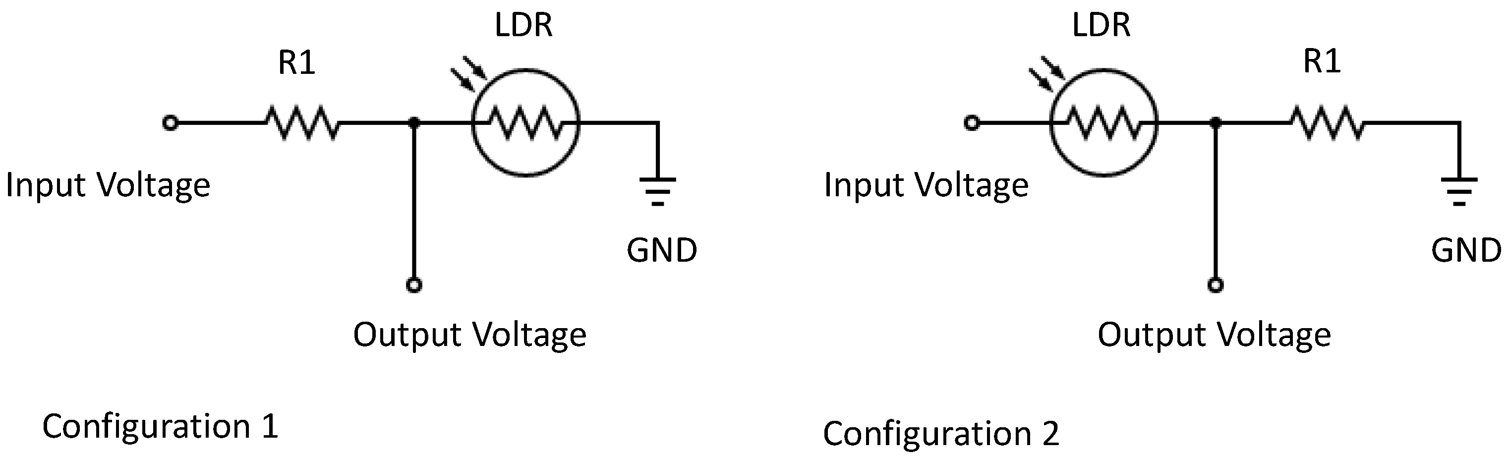
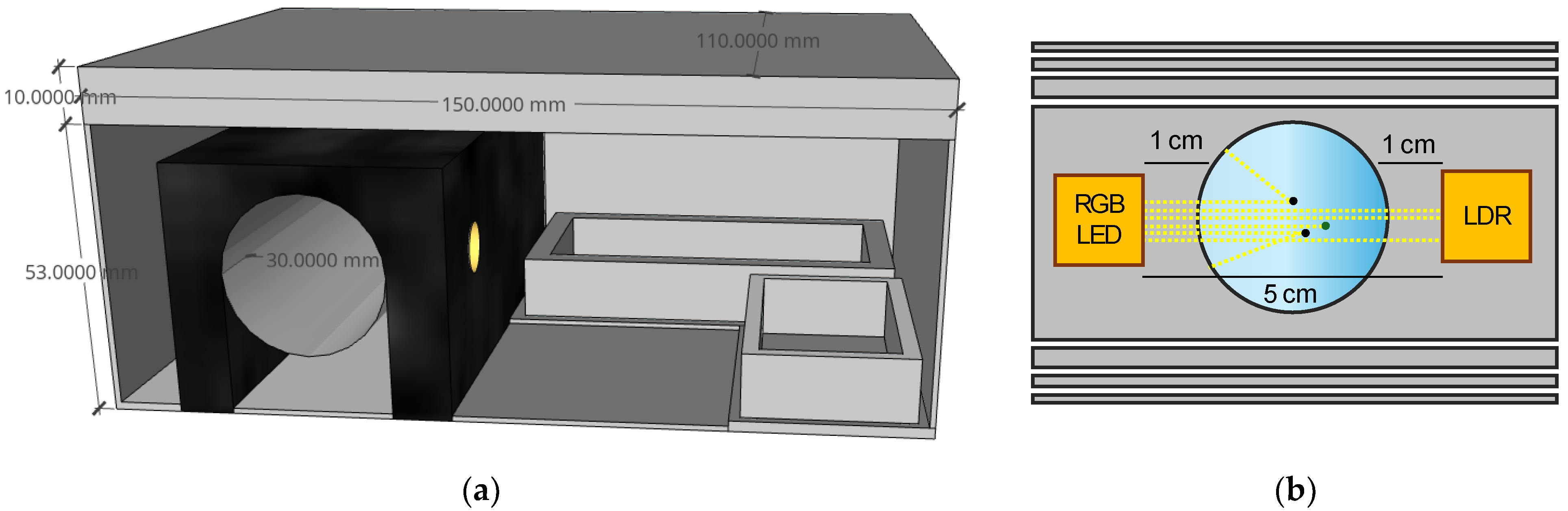
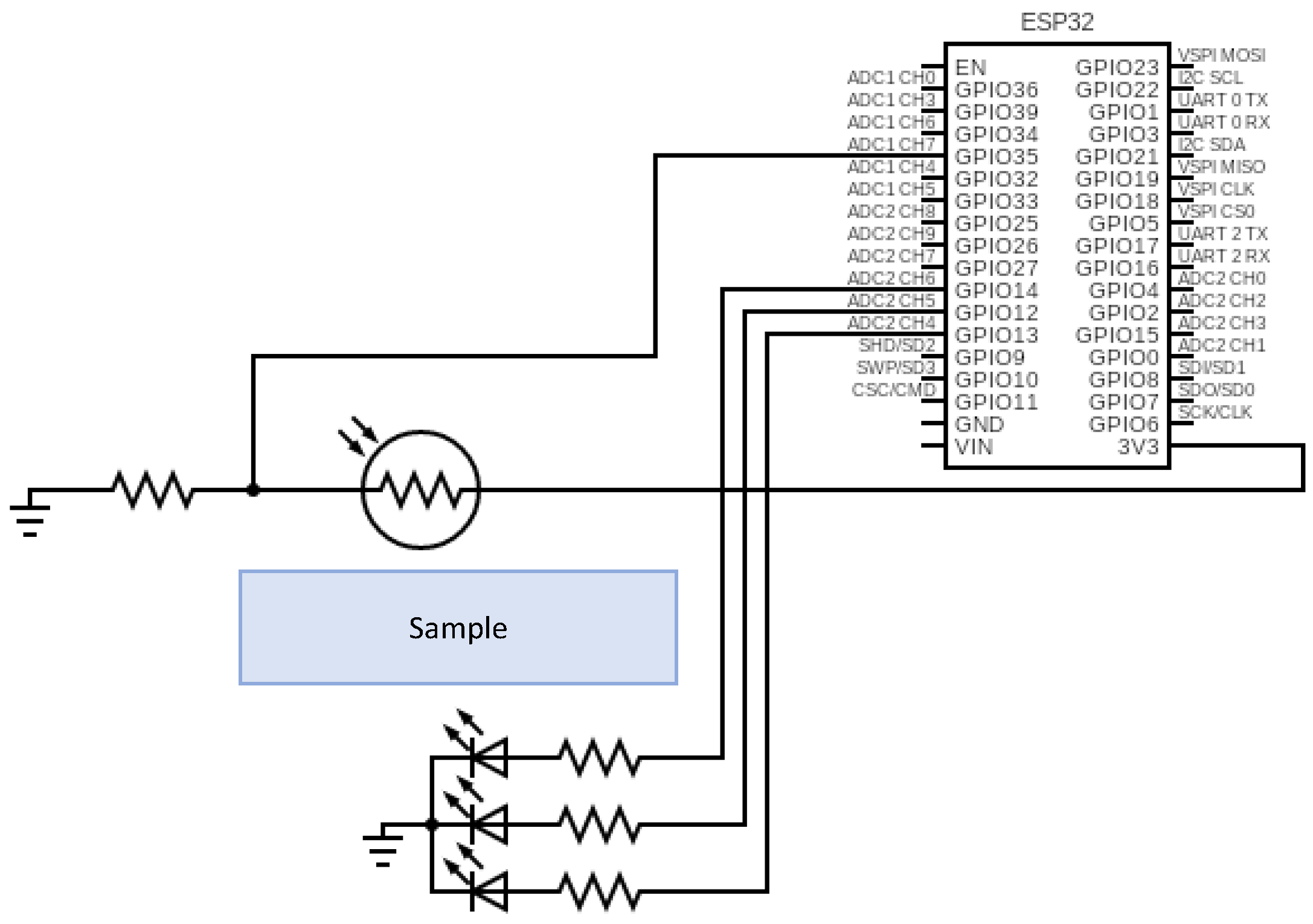
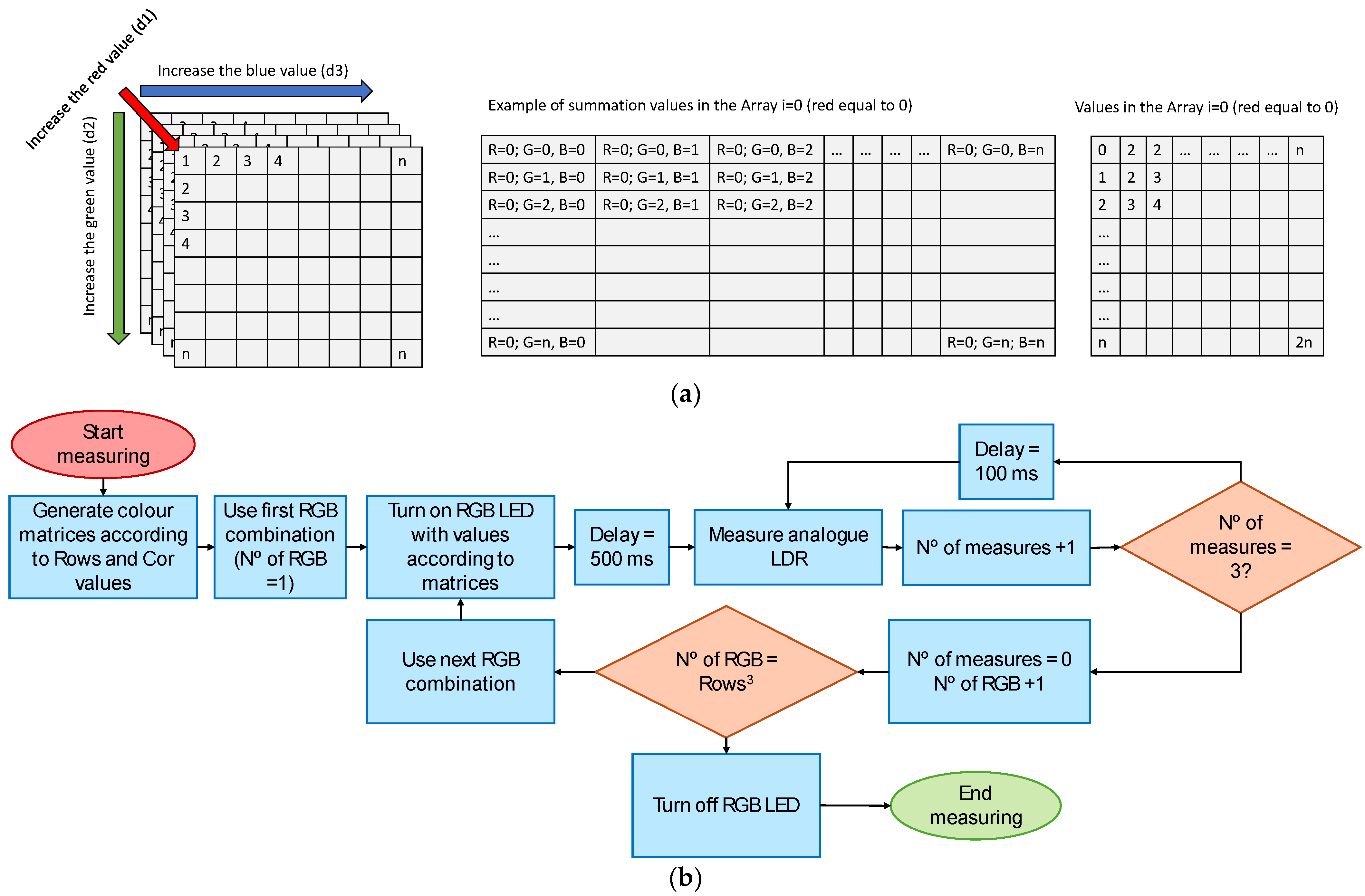
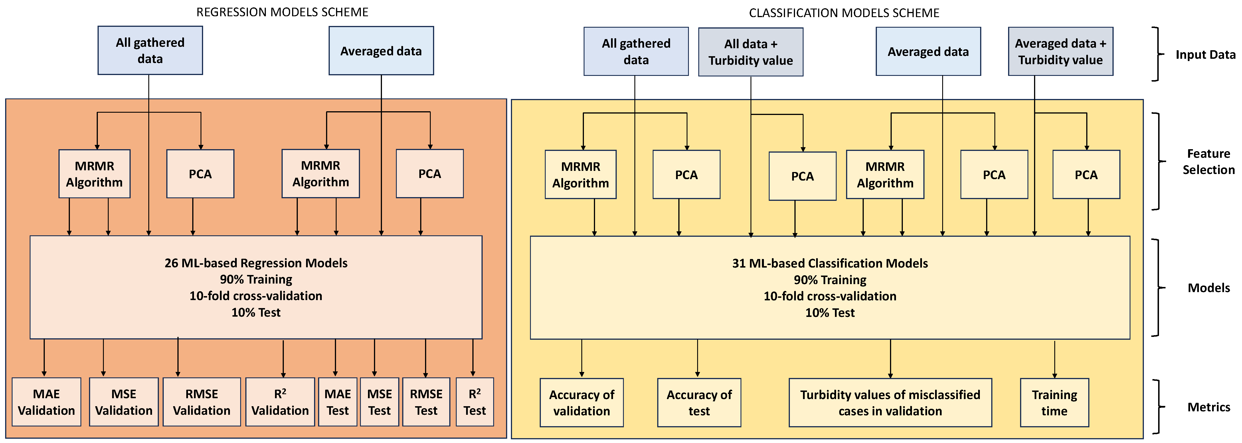
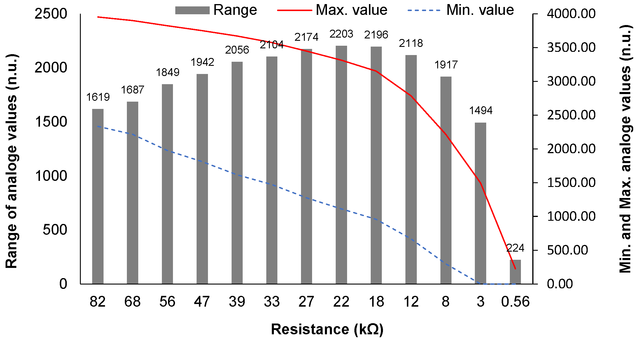
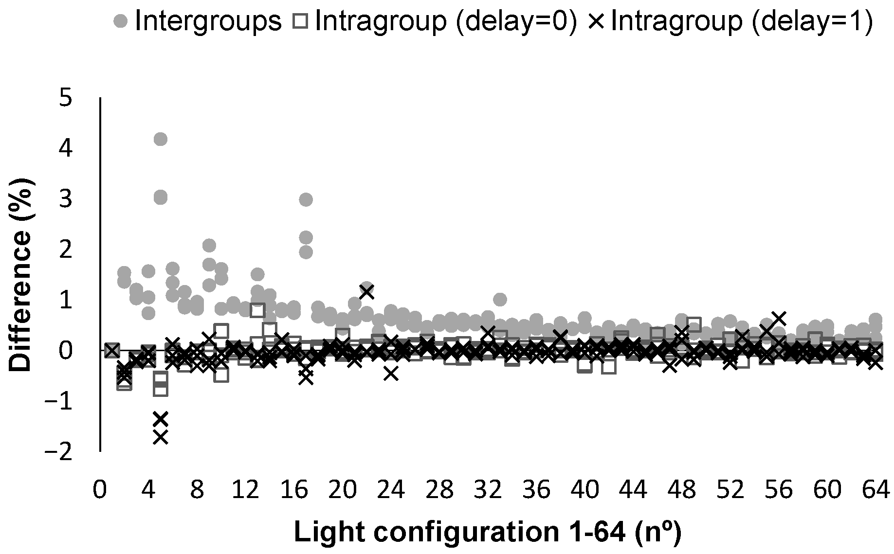
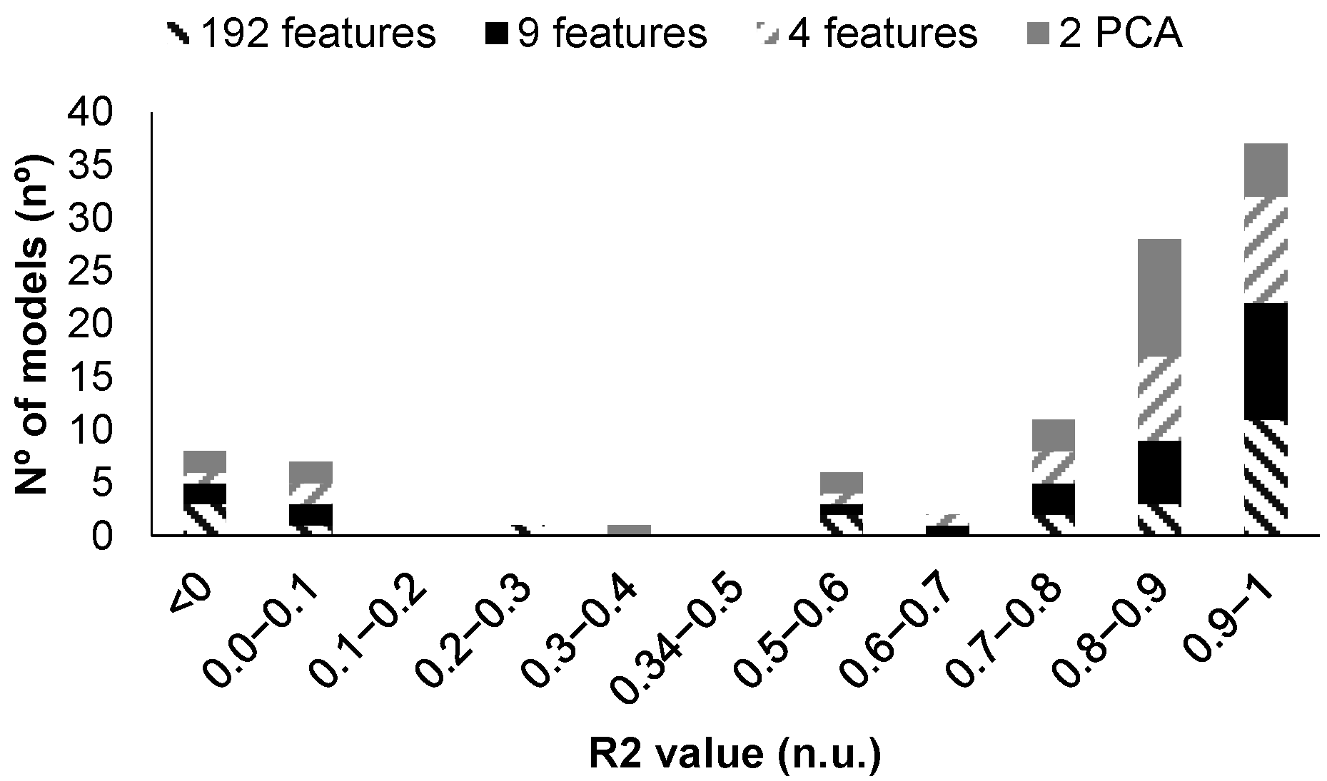
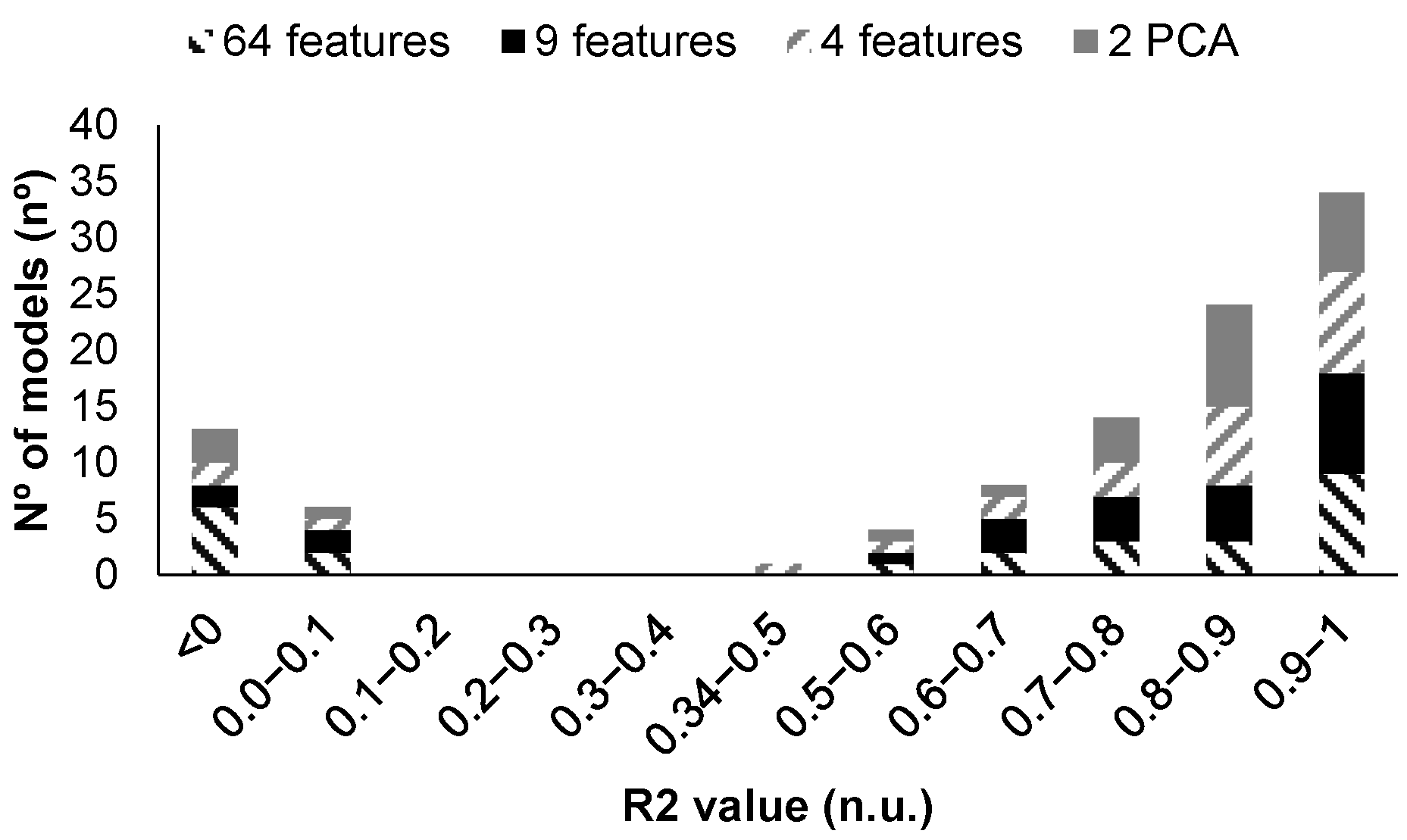
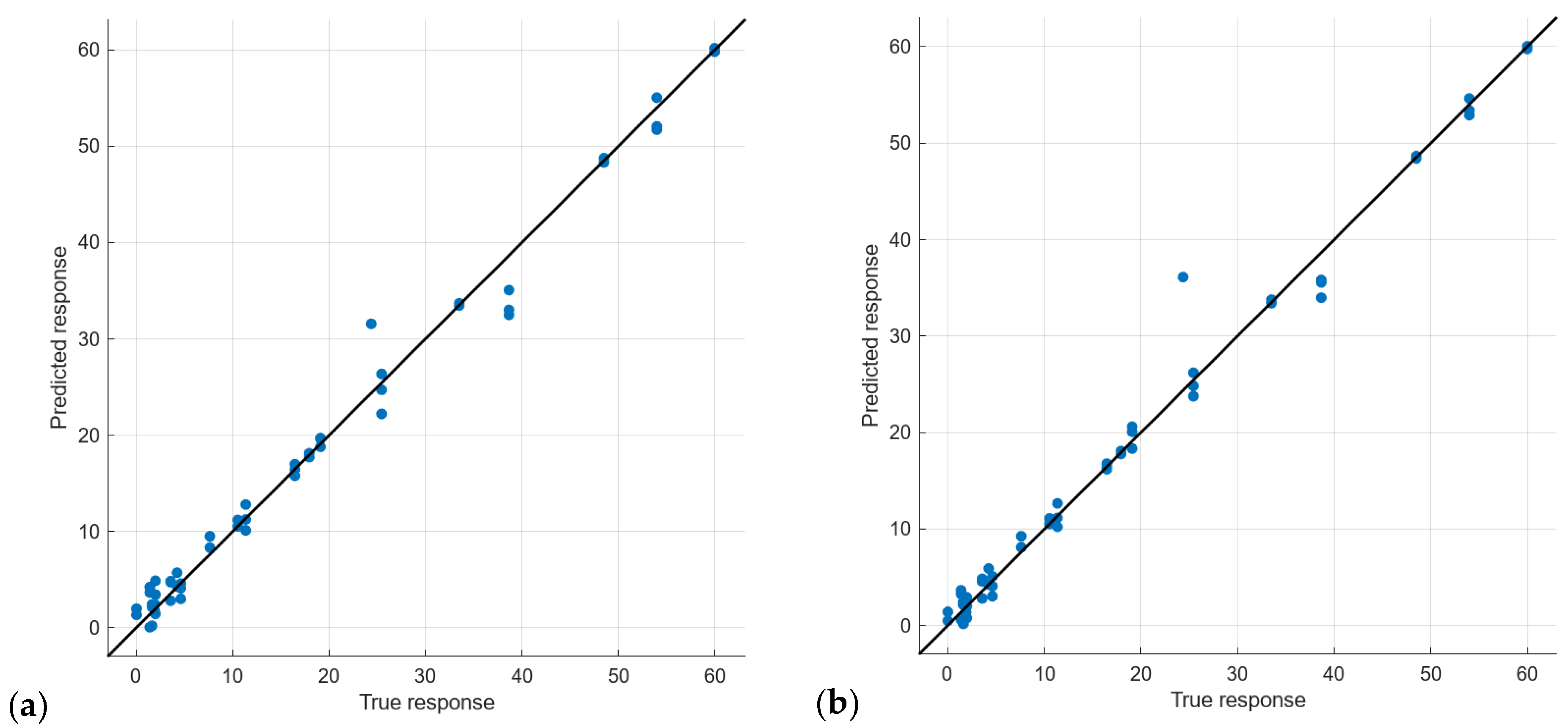
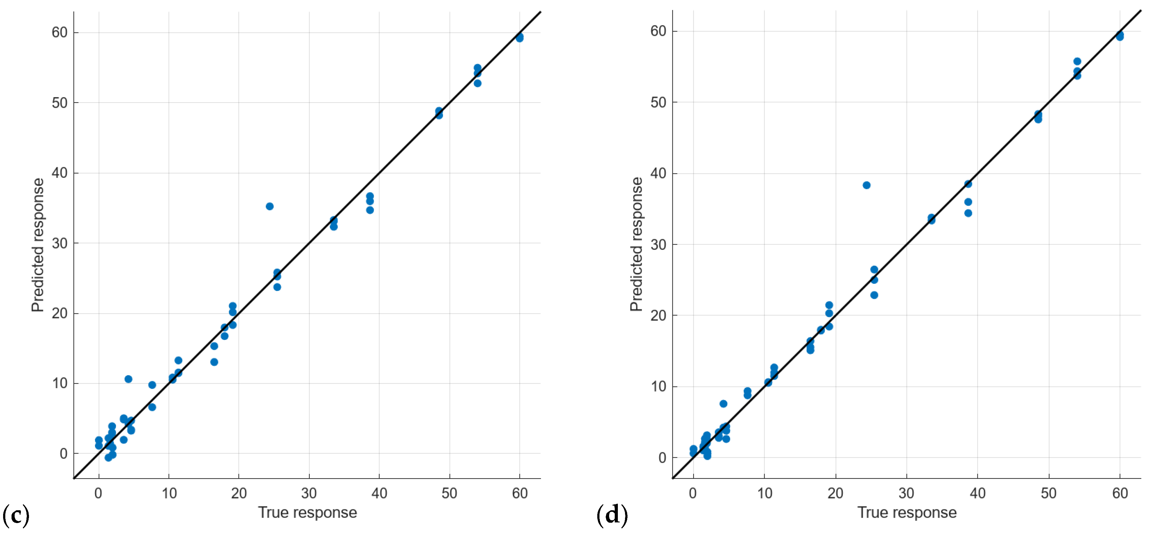
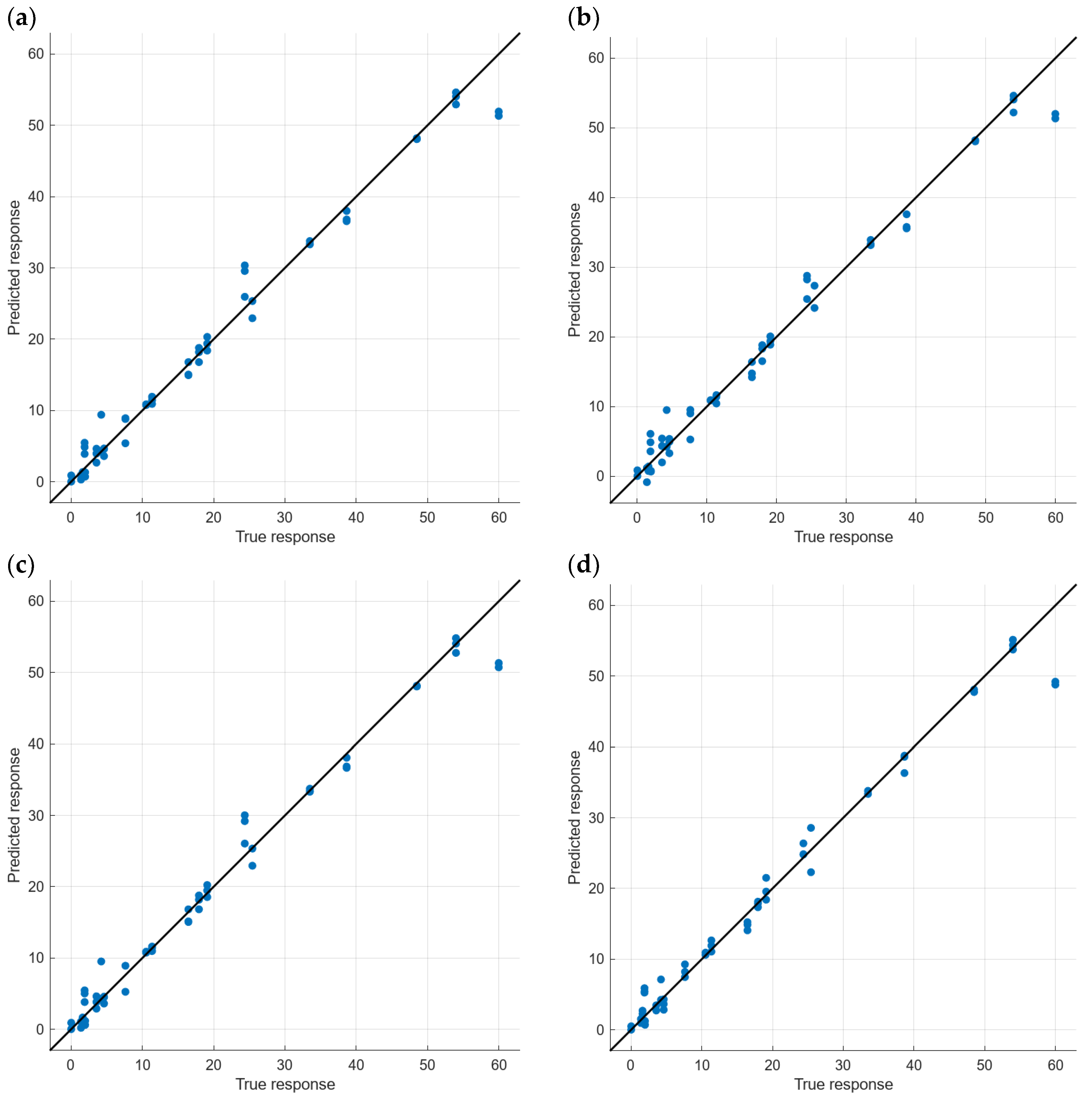
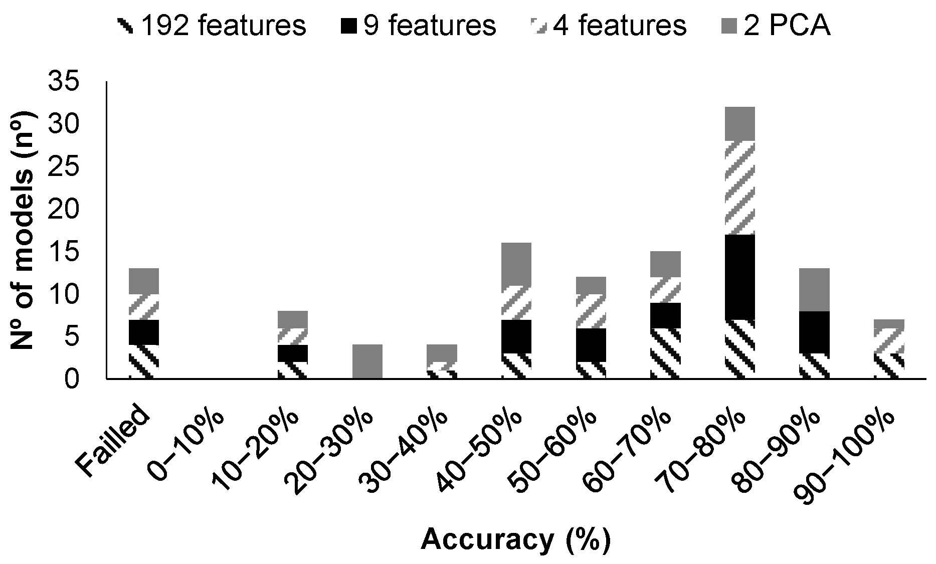
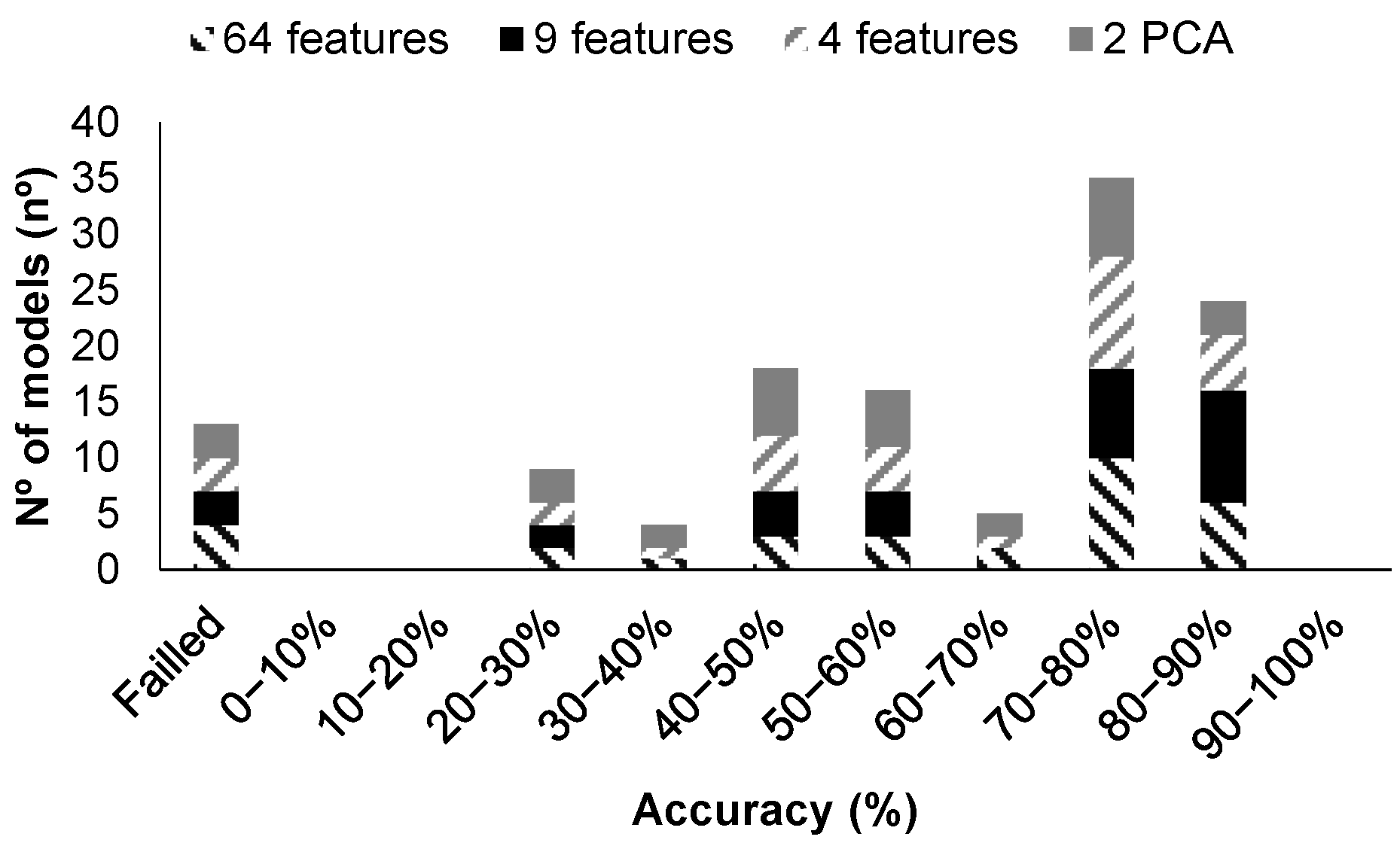
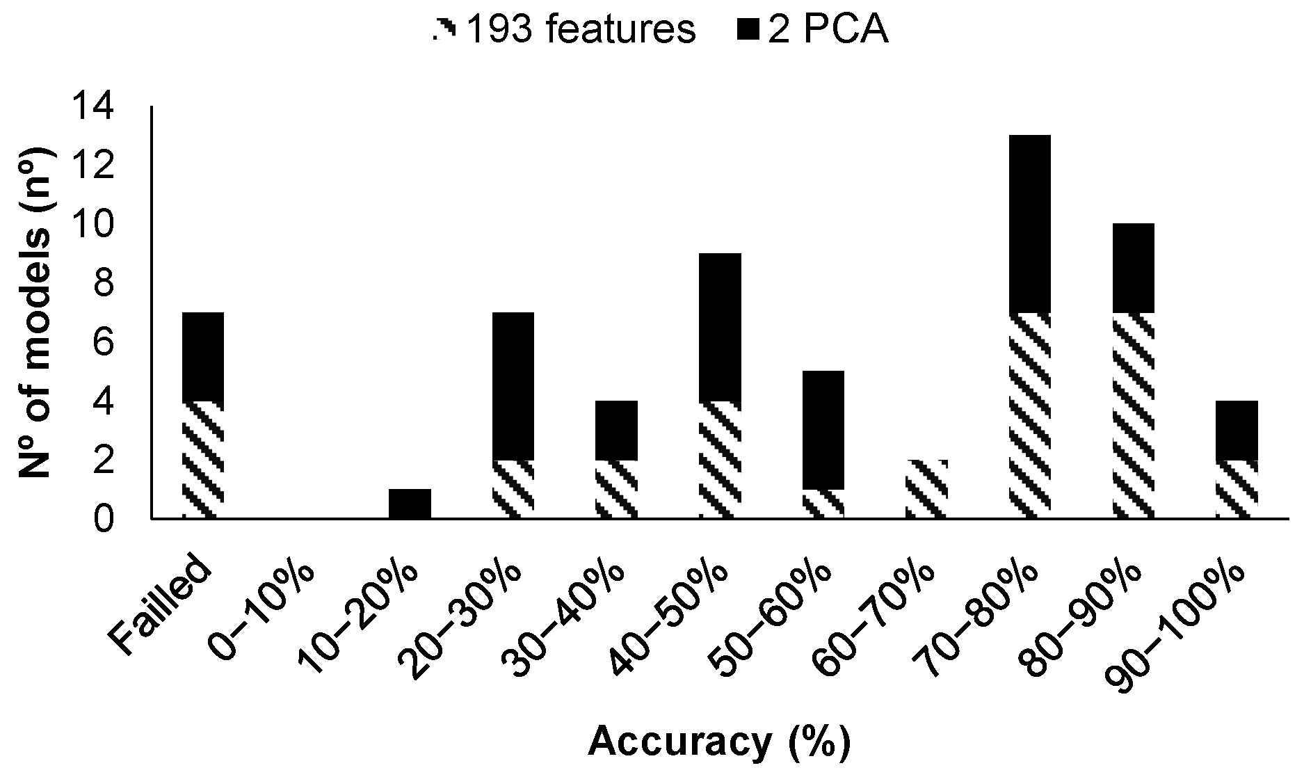
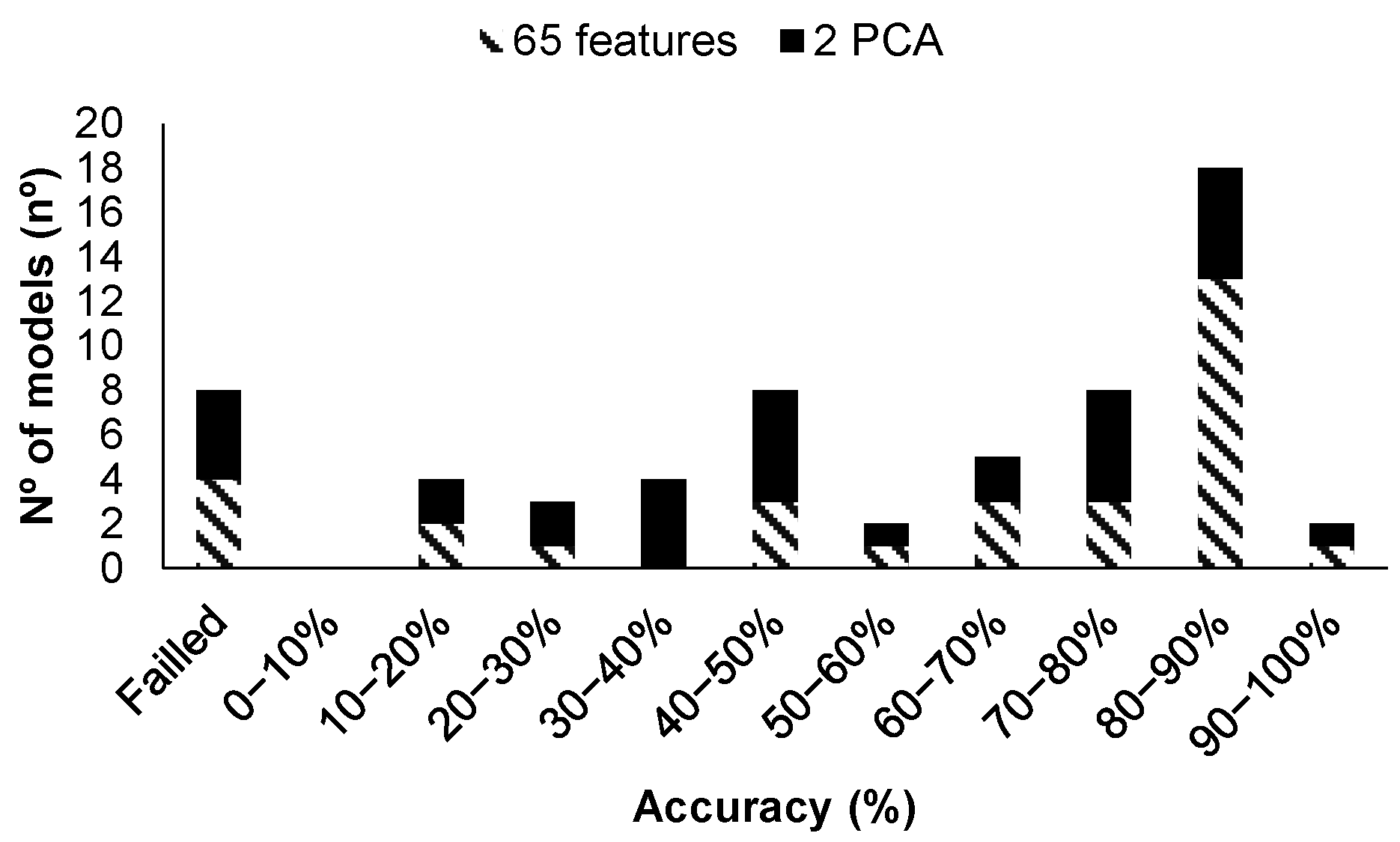
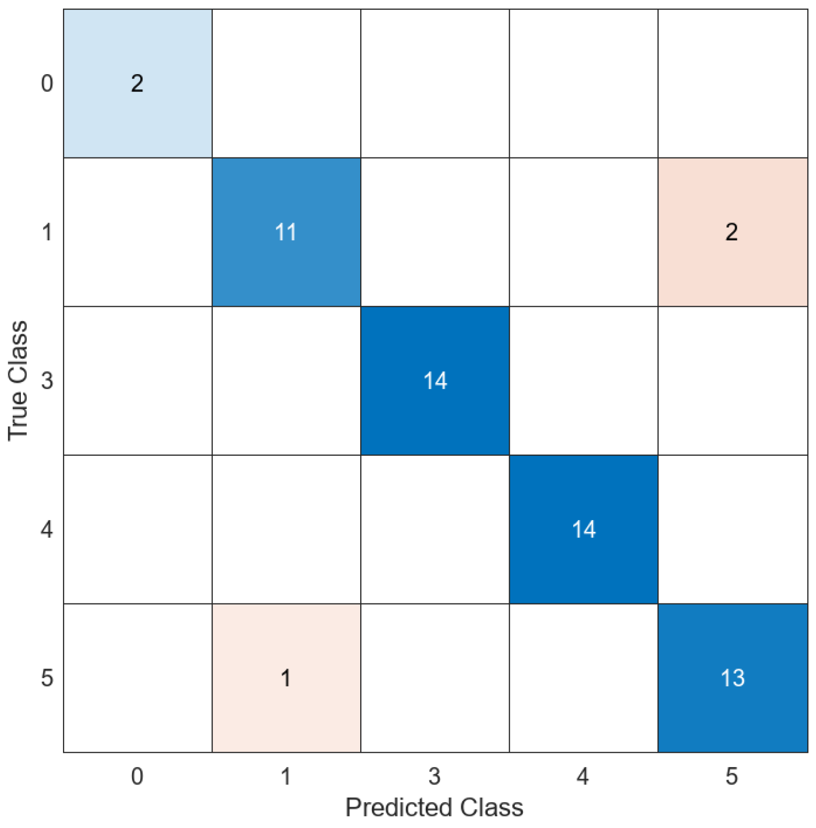
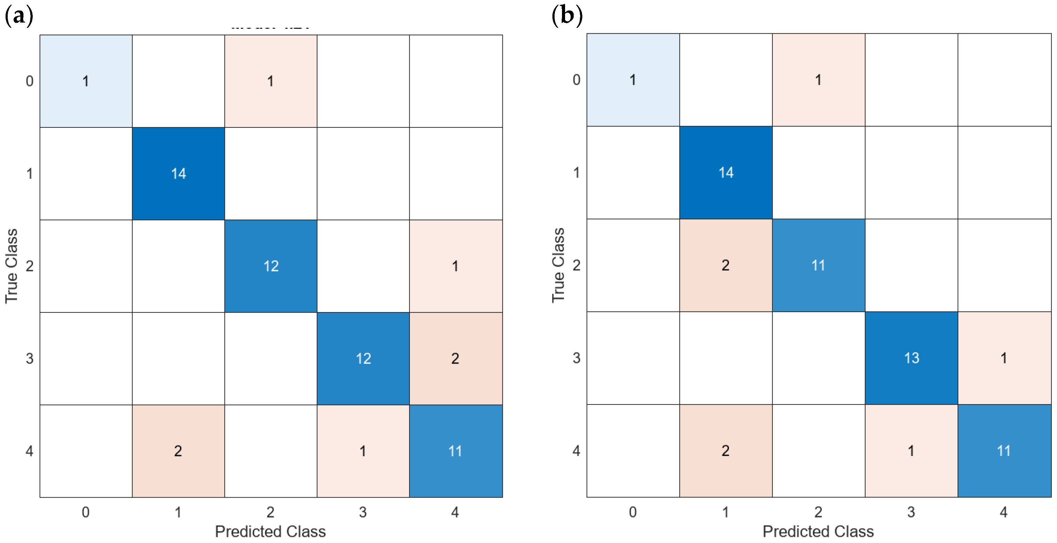
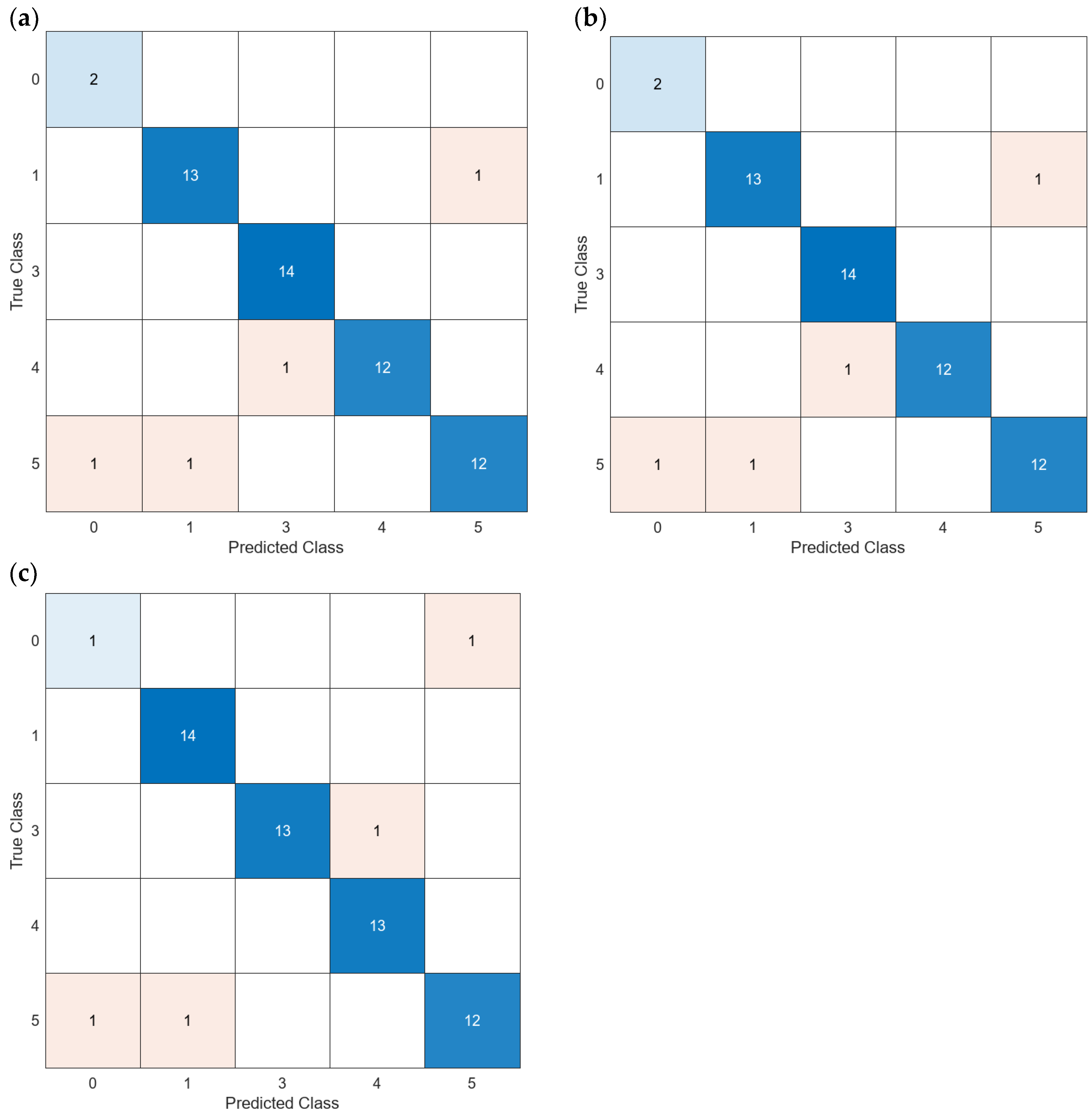
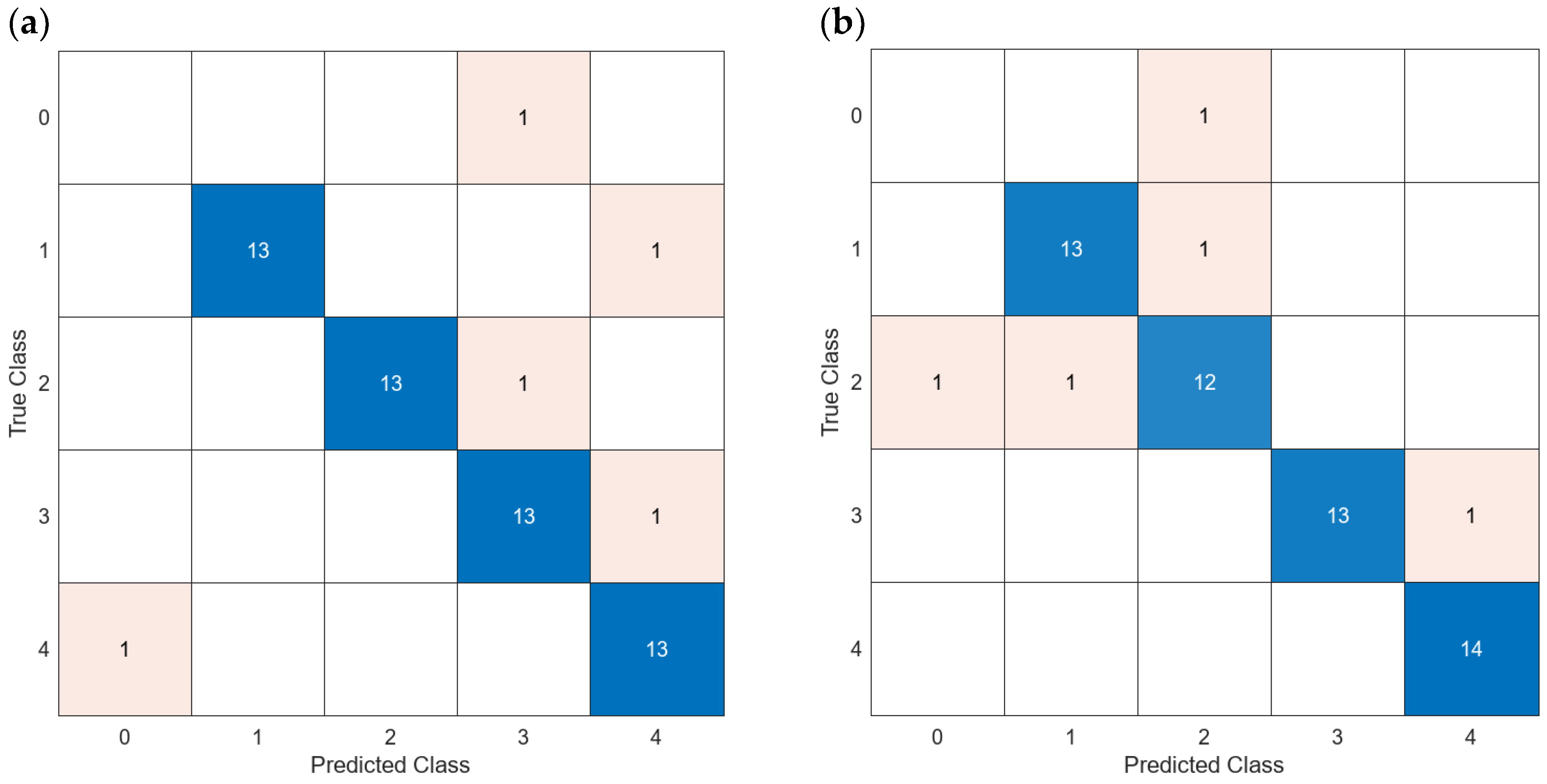
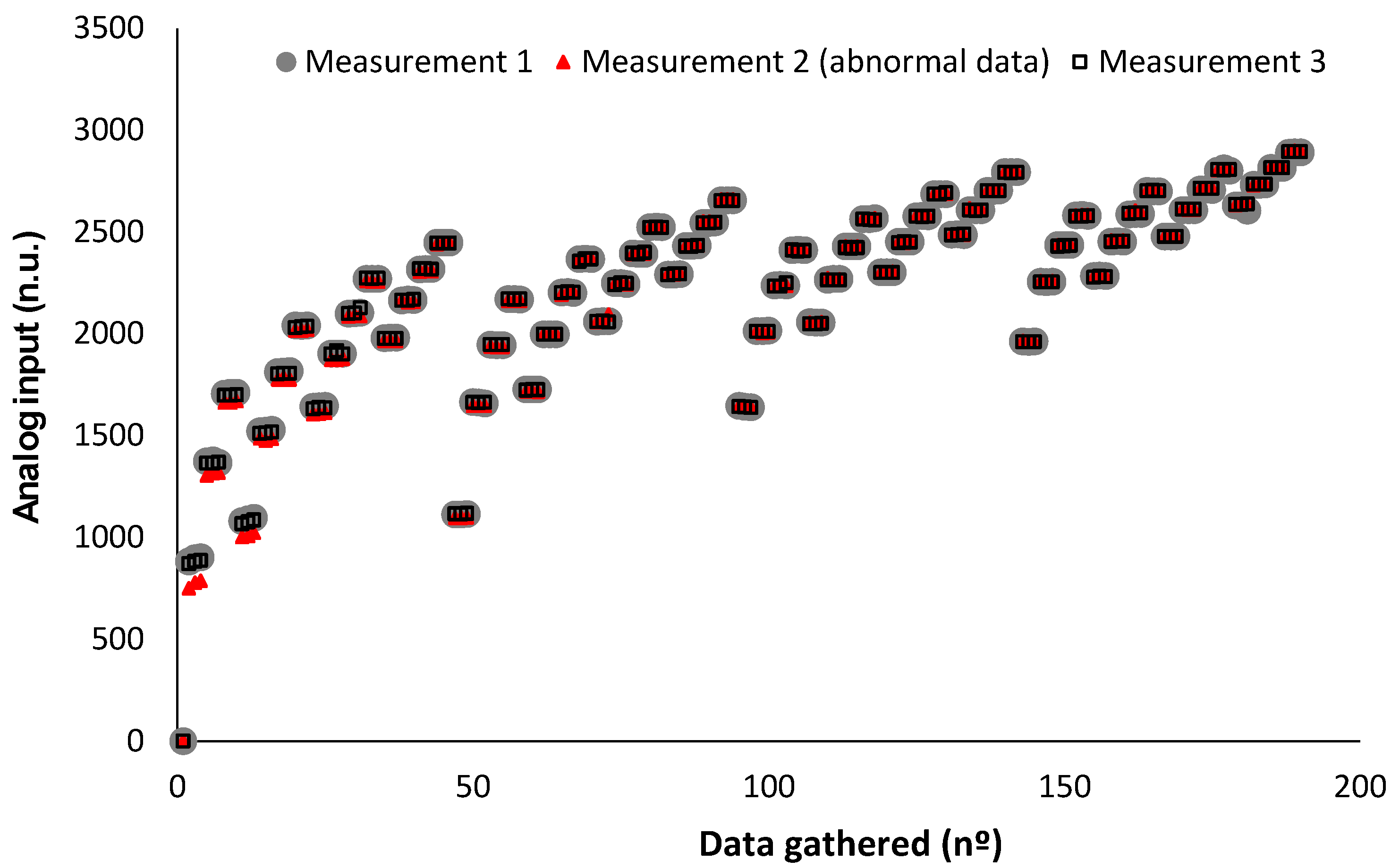
Table 1.
Required minimum time for measuring the different light combinations.
| Rows (nº) | Total Light Combinations (nº) | Required Time for Complete Measurement (s) |
|---|---|---|
| 3 | 27 | 13.5 |
| 4 | 64 | 32 |
| 5 | 125 | 62.5 |
| 6 | 216 | 108 |
| 7 | 343 | 171.5 |
| 8 | 512 | 256 |
| 9 | 729 | 364.5 |
| 10 | 1000 | 500 |
Table 2.
Values to be used to power each LED, according to the different matrix sizes.
| Rows (nº) | Cor Value (nº) | Values | |||||||||
|---|---|---|---|---|---|---|---|---|---|---|---|
| 3 | 84 | 0 | 84 | 168 | |||||||
| 4 | 63 | 0 | 63 | 126 | 189 | ||||||
| 5 | 50 | 0 | 50 | 100 | 150 | 200 | |||||
| 6 | 42 | 0 | 42 | 84 | 126 | 168 | 210 | ||||
| 7 | 35 | 0 | 35 | 70 | 105 | 140 | 175 | 210 | |||
| 8 | 31 | 0 | 31 | 62 | 93 | 124 | 155 | 186 | 217 | ||
| 9 | 27 | 0 | 27 | 54 | 81 | 108 | 135 | 162 | 189 | 216 | |
| 10 | 25 | 0 | 25 | 50 | 75 | 100 | 125 | 150 | 175 | 200 | 225 |
Table 3.
Details and turbidity values of the generated samples.
| Id | Label | Added Solid | Dilution | Turbidity in t = 0 min (NTUs) | Turbidity in t = 1 min (NTUs) |
|---|---|---|---|---|---|
| 1 | a | fresh green vegetal organic matter | 60 | 53 | 38.66 |
| 2 | a | 33.33 | 25.66 | 19.1 | |
| 3 | a | 20 | 11.37 | 10.53 | |
| 4 | a | 11.11 | 5.25 | 4.23 | |
| 5 | a | 3.45 | 1.99 | 1.62 | |
| 6 | b | decaying vegetal organic matter | 15 | 53 | 54 |
| 7 | b | 10 | 26.69 | 24.37 | |
| 8 | b | 5 | 11.72 | 11.36 | |
| 9 | b | 2.5 | 8.45 | 7.62 | |
| 10 | b | 0.72 | 2.62 | 1.9 | |
| 11 | c | soil and ashes | 10 | 50 | 48.51 |
| 12 | c | 8 | 25.86 | 25.44 | |
| 13 | c | 5 | 16.98 | 16.46 | |
| 14 | c | 2.5 | 4.59 | 3.73 | |
| 15 | c | 0.84 | 2.65 | 1.97 | |
| 16 | d | soil | 15 | 66 | 60 |
| 17 | d | 10 | 37.25 | 33.5 | |
| 18 | d | 5 | 18.39 | 17.94 | |
| 19 | d | 2.5 | 6.21 | 3.56 | |
| 20 | d | 1.25 | 1.83 | 2.51 | |
| 21 | - | - | - | 0.74 | 0.02 |
Table 4.
Type of models to be used in the regression.
| Id | Type of Model | Preset | Id | Type of Model | Preset |
|---|---|---|---|---|---|
| 1 | LR | Linear | 14 | Ensemble | Boosted Trees |
| 2 | LR | Interactions Linear | 15 | Ensemble | Bagged Trees |
| 3 | LR | Robust Linear | 16 | GPR | Squared Exponential GPR |
| 4 | Stepwise LR | Stepwise Linear | 17 | GPR | Matern 5/2 GPR |
| 5 | Tree | Fine Tree | 18 | GPR | Exponential GPR |
| 6 | Tree | Medium Tree | 19 | GPR | Rational Quadratic GPR |
| 7 | Tree | Coarse Tree | 20 | NN | Narrow Neural Network |
| 8 | SVM | Linear SVM | 21 | NN | Medium Neural Network |
| 9 | SVM | Quadratic SVM | 22 | NN | Wide Neural Network |
| 10 | SVM | Cubic SVM | 23 | NN | Bilayered Neural Network |
| 11 | SVM | Fine Gaussian SVM | 24 | NN | Trilayered Neural Network |
| 12 | SVM | Medium Gaussian SVM | 25 | Kernel | SVM Kernel |
| 13 | SVM | Coarse Gaussian SVM | 26 | Kernel | Least Squares Regression Kernel |
Table 5.
Type of models to be used in the classification.
| Id | Type of Model | Preset | Id | Type of Model | Preset |
|---|---|---|---|---|---|
| 1 | Tree | Fine Tree | 17 | KNN | Cosine KNN |
| 2 | Tree | Medium Tree | 18 | KNN | Cubic KNN |
| 3 | Tree | Coarse Tree | 19 | KNN | Weighted KNN |
| 4 | Discriminant | Linear Discriminant | 20 | Ensemble | Boosted Trees |
| 5 | Discriminant | Quadratic Discriminant | 21 | Ensemble | Bagged Trees |
| 6 | Naive Bayes | Gaussian Naive Bayes | 22 | Ensemble | Subspace Discriminant |
| 7 | Naive Bayes | Kernel Naive Bayes | 23 | Ensemble | Subspace KNN |
| 8 | SVM | Linear SVM | 24 | Ensemble | RUSBoosted Trees |
| 9 | SVM | Quadratic SVM | 25 | NN | Narrow Neural Network |
| 10 | SVM | Cubic SVM | 26 | NN | Medium Neural Network |
| 11 | SVM | Fine Gaussian SVM | 27 | NN | Wide Neural Network |
| 12 | SVM | Medium Gaussian SVM | 28 | NN | Bilayered Neural Network |
| 13 | SVM | Coarse Gaussian SVM | 29 | NN | Trilayered Neural Network |
| 14 | KNN | Fine KNN | 30 | Kernel | SVM Kernel |
| 15 | KNN | Medium KNN | 31 | Kernel | Logistic Regression Kernel |
| 16 | KNN | Coarse KNN |
Table 6.
The rest of the metrics are for the validation and testing of selected models of regression models with all data.
Table 6.
The rest of the metrics are for the validation and testing of selected models of regression models with all data.
| Model Id | Used Features | Label in Figure 10 | RMSE Validation | MSE Validation | MAE Validation | RMSE Test | MSE Test | MAE Test |
|---|---|---|---|---|---|---|---|---|
| 17 | 192 | (a) | 1.92 | 3.68 | 1.20 | 0.70 | 0.50 | 0.47 |
| 19 | PCA | (b) | 1.97 | 3.86 | 1.03 | 0.81 | 0.66 | 0.61 |
| 16 | 192 | (c) | 2.18 | 4.76 | 1.35 | 1.44 | 2.09 | 1.20 |
| 18 | PCA | (d) | 2.21 | 4.89 | 1.07 | 1.33 | 1.78 | 0.90 |
Table 7.
The rest of the metrics are for the validation and testing of selected models of regression models with averaged data.
Table 7.
The rest of the metrics are for the validation and testing of selected models of regression models with averaged data.
| Model Id | Used Features | Label in Figure 11 | RMSE Validation | MSE Validation | MAE Validation | RMSE Test | MSE Test | MAE Test |
|---|---|---|---|---|---|---|---|---|
| 17 | 192 | (a) | 2.29 | 5.25 | 1.34 | 0.70 | 0.75 | 0.86 |
| 19 | PCA | (b) | 2.30 | 5.30 | 1.48 | 0.90 | 1.02 | 1.01 |
| 16 | 192 | (c) | 2.35 | 5.51 | 1.34 | 0.63 | 0.68 | 0.83 |
| 18 | PCA | (d) | 2.49 | 6.19 | 1.31 | 0.55 | 0.47 | 0.68 |
Table 8.
The rest of the metrics are for the validation and testing of selected models of classification models.
Table 8.
The rest of the metrics are for the validation and testing of selected models of classification models.
| Model Id | Averaged or All Data | Used Turbidity | Used Features | Turbidity of Misclassified Data Validation (NTUs) | Figure and Label | Accuracy Test (%) | Training Time (s) |
|---|---|---|---|---|---|---|---|
| 14 | All | No | 192 | <5 | Figure 16 | 83.33 | 1.6975015 |
| 21 | Averaged | No | 3 | <50 | Figure 17a | 100 | 2.545574 |
| 21 | Averaged | No | 64 PCA | <50 | Figure 17b | 100 | 3.1462531 |
| 14 | All | Yes | 192 | 4.62 | Figure 18a | 100 | 2.6324913 |
| 23 | All | Yes | 192 | 4.62 | Figure 18b | 100 | 5.2588926 |
| 14 | All | Yes | 192 PCA | 4.62 | Figure 18c | 100 | 1.9605995 |
| 27 | Averaged | Yes | 65 | 11.36 | Figure 19a | 83.33 | 1.8494421 |
| 14 | Averaged | Yes | 65 PCA | 4.62 | Figure 19b | 100 | 1.1472791 |
Table 9.
Comparison of the proposed sensor with the state-of-the-art models (I): Quantify the turbidity.
Table 9.
Comparison of the proposed sensor with the state-of-the-art models (I): Quantify the turbidity.
| Year | Used Lights | Min. Max. Values (NTUS) | Samples < 5 NTU | Adjust Resistances | Regression Model | R2 | MAE (NTU) | MSE (%) | RMSE (%) | Ref. |
|---|---|---|---|---|---|---|---|---|---|---|
| 2016 | Red LED | 10–85 | No | Simple Regression | 0.959 | 8.02 | [48] | |||
| 2018 | IR LED | 0–200 | No | Simple Regression | 10 | [30] | ||||
| 2019 | Cubert UHD 285 | 0–4 * | Yes | SVM + PCA | 0.902 | 0.2 | [49] | |||
| 2019 | IR LED | 0–80 * | No | Simple Regression | 0.943 | [50] | ||||
| 2020 | Visible IR light | 0–4000 | No | Yes | EMG | [25] | ||||
| 2022 | IR | 20–4000 | No | Simple Regression | 10 | 10 | [51] | |||
| 2023 | IR + RGB LED | 2.73–176.7 | Yes | Yes | NN | 0.983 | 2.85 | 7.45 | [29] | |
| 2024 | RGB LED | 0.2–60 | Yes | Yes | Exponential GPR + PCA | 0.979 | 0.68 | 0.47 | 0.55 | Proposed |
Table 10.
Comparison of the proposed sensor with the state-of-the-art models (II): Characterise the turbidity.
Table 10.
Comparison of the proposed sensor with the state-of-the-art models (II): Characterise the turbidity.
| Year | Used Lights | Nº of Classes | Classification Model | Accuracy (%) | Maximum Values Misclassified | Ref. |
|---|---|---|---|---|---|---|
| 2018 | IR + RGB | 4 Turbidity sources | Based on regression models and algorithms | - | [19] | |
| 2021 | IR + RGB | 2 Turbidity sources | Based on regression models and algorithms | - | [56] | |
| 2023 | IR + RGB | 2 Turbidity sources | NN | 90.9 | - | [29] |
| 2022 | Landsat 8 | 5 Levels of turbidity | Random Forest | 85 | - | [52] |
| 2023 | Sentinel 2 | 2 Levels of turbidity | Isolated Forest | 89.58 | [53] | |
| 2023 | Image in Laboratory | 5 Levels of turbidity | Deep Learning | 97.5 | [54] | |
| 2022 | Image in laboratory with different lights | 9 Levels or turbidity | CNN | 100 | [55] | |
| 2024 | 64 visible lights | 4 Turbidity sources | Fine KNN | 91.23 | <5 NTUs | Proposal |
Disclaimer/Publisher’s Note: The statements, opinions and data contained in all publications are solely those of the individual author(s) and contributor(s) and not of MDPI and/or the editor(s). MDPI and/or the editor(s) disclaim responsibility for any injury to people or property resulting from any ideas, methods, instructions or products referred to in the content. |
© 2024 by the authors. Licensee MDPI, Basel, Switzerland. This article is an open access article distributed under the terms and conditions of the Creative Commons Attribution (CC BY) license (https://creativecommons.org/licenses/by/4.0/).
Share and Cite
MDPI and ACS Style
Parra, L.; Ahmad, A.; Sendra, S.; Lloret, J.; Lorenz, P. Combination of Machine Learning and RGB Sensors to Quantify and Classify Water Turbidity. Chemosensors 2024, 12, 34. https://doi.org/10.3390/chemosensors12030034
AMA Style
Parra L, Ahmad A, Sendra S, Lloret J, Lorenz P. Combination of Machine Learning and RGB Sensors to Quantify and Classify Water Turbidity. Chemosensors. 2024; 12(3):34. https://doi.org/10.3390/chemosensors12030034
Chicago/Turabian StyleParra, Lorena, Ali Ahmad, Sandra Sendra, Jaime Lloret, and Pascal Lorenz. 2024. "Combination of Machine Learning and RGB Sensors to Quantify and Classify Water Turbidity" Chemosensors 12, no. 3: 34. https://doi.org/10.3390/chemosensors12030034
Note that from the first issue of 2016, this journal uses article numbers instead of page numbers. See further details here.