
Using Deep Convolutional Neural Network for Image-Based Diagnosis of Nutrient Deficiencies in Plants Grown in Aquaponics


 ,
,  ,
,  , ,
, ,  ,
,  and
and
Abstract
:1. Introduction
2. Materials and Methods
2.1. Chemicals and Materials
2.2. Chemical Analysis
2.3. Experimental Setup
2.4. Spectral Reflectance Measurement of Lettuce Leaves
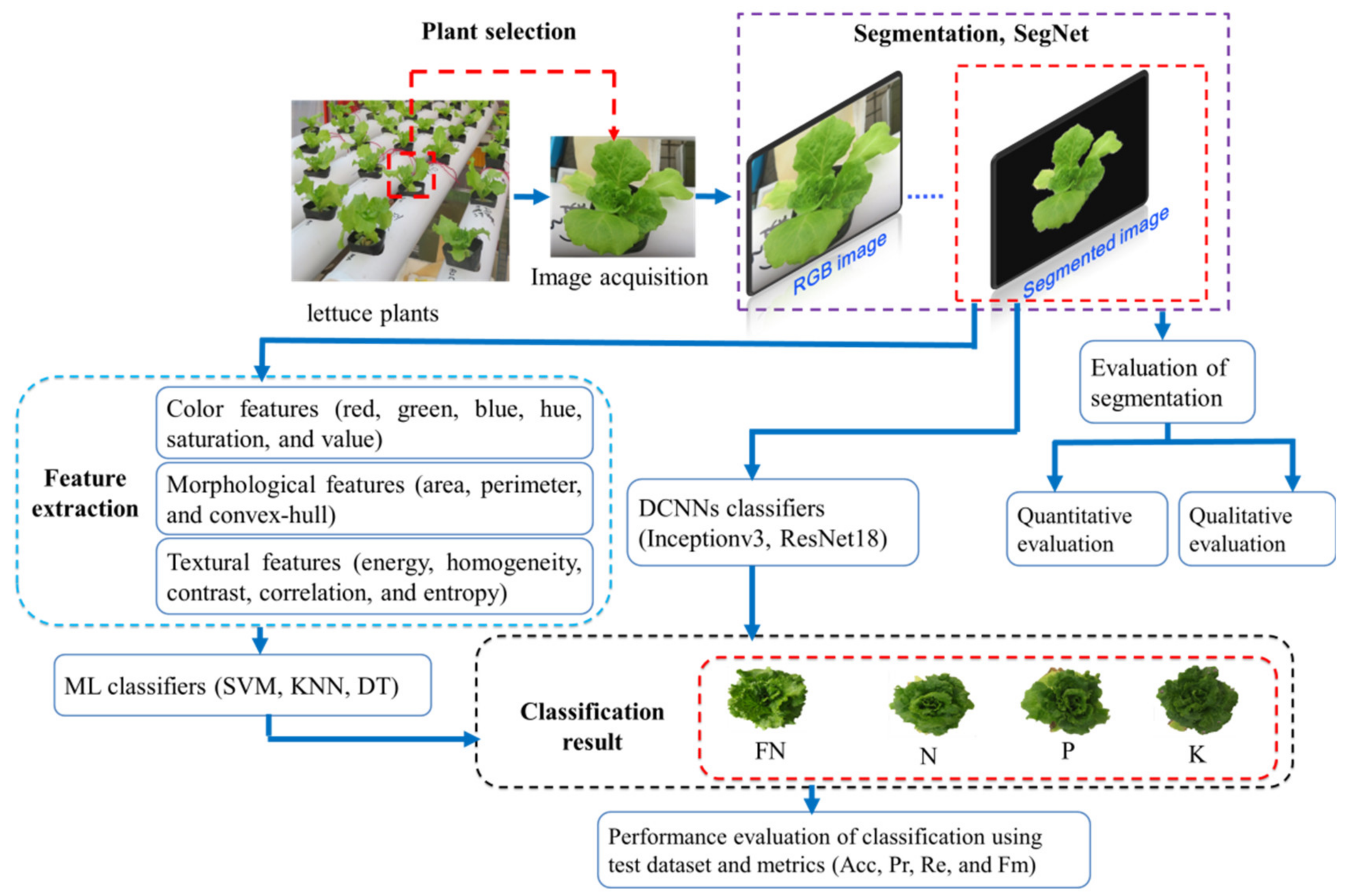
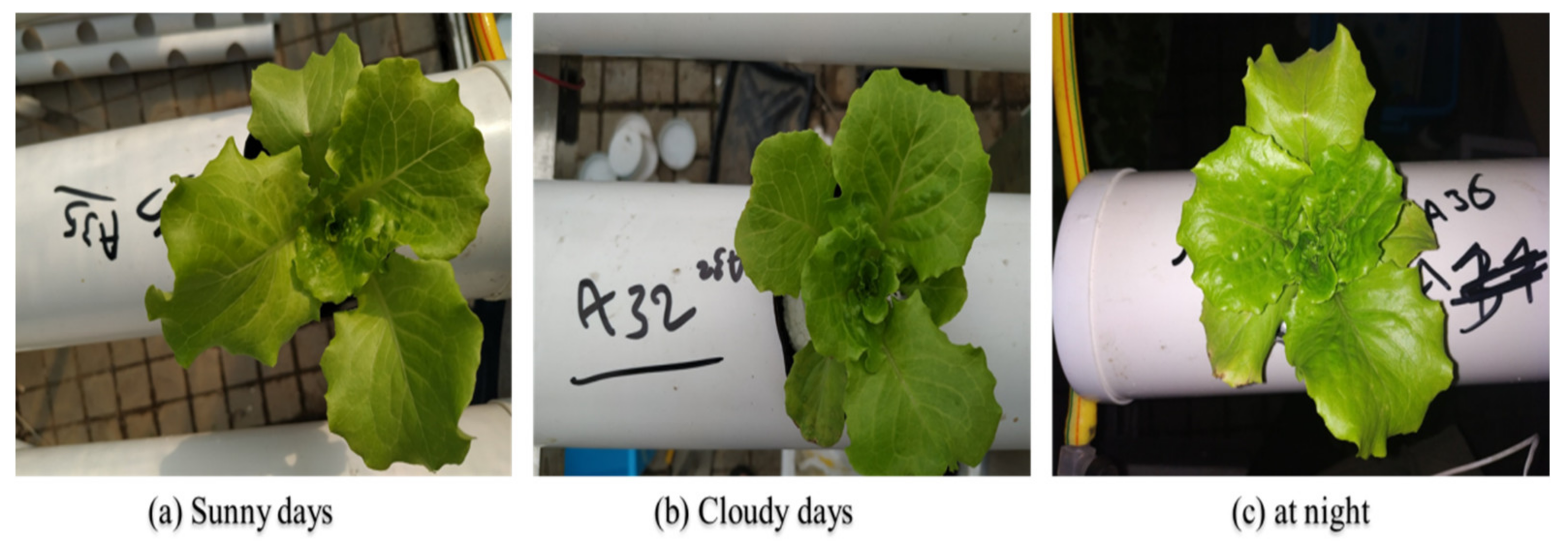
2.5. Image Acquisition
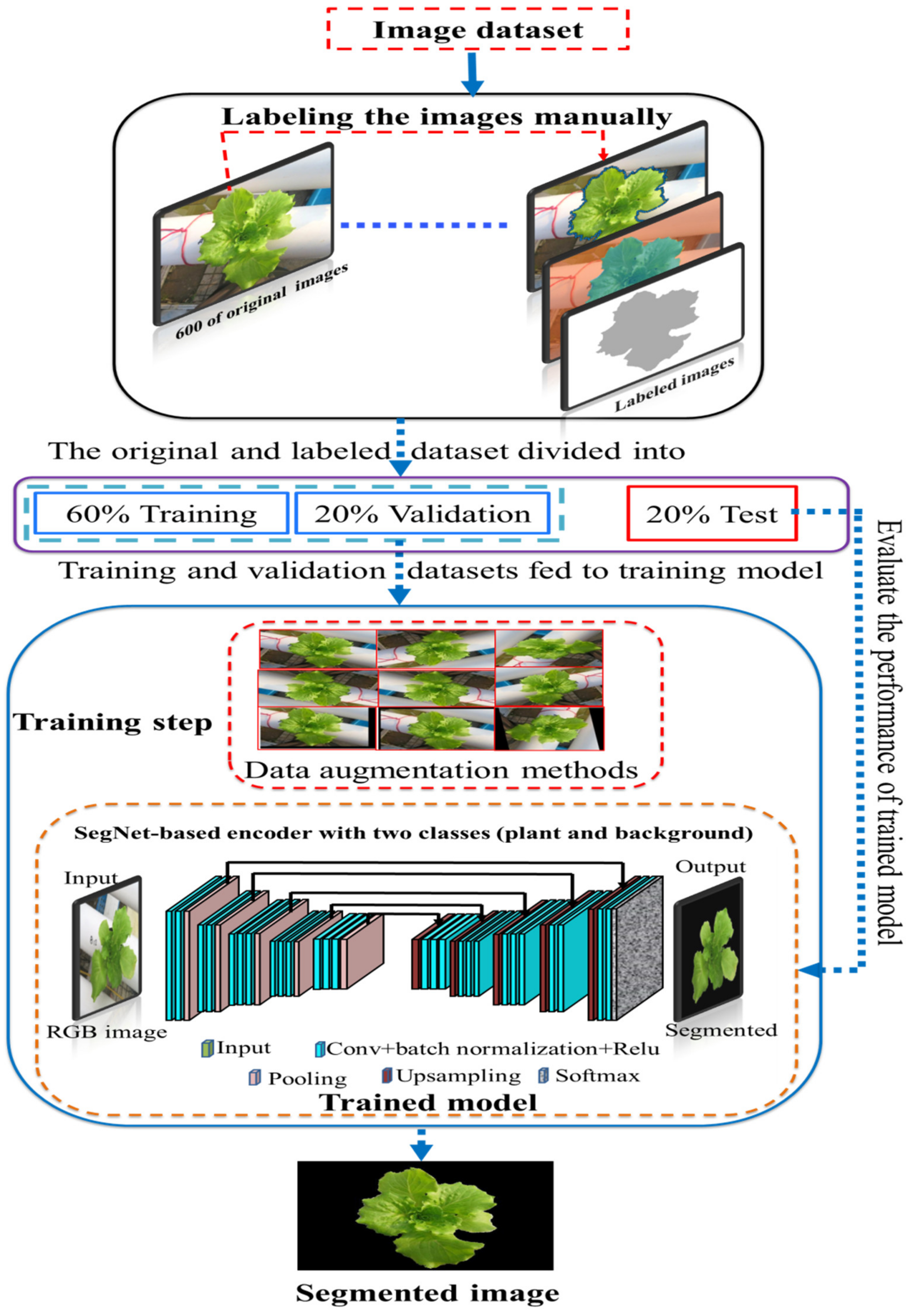
2.6. Image Segmentation
2.7. Feature Extraction
2.8. Traditional ML Classifiers
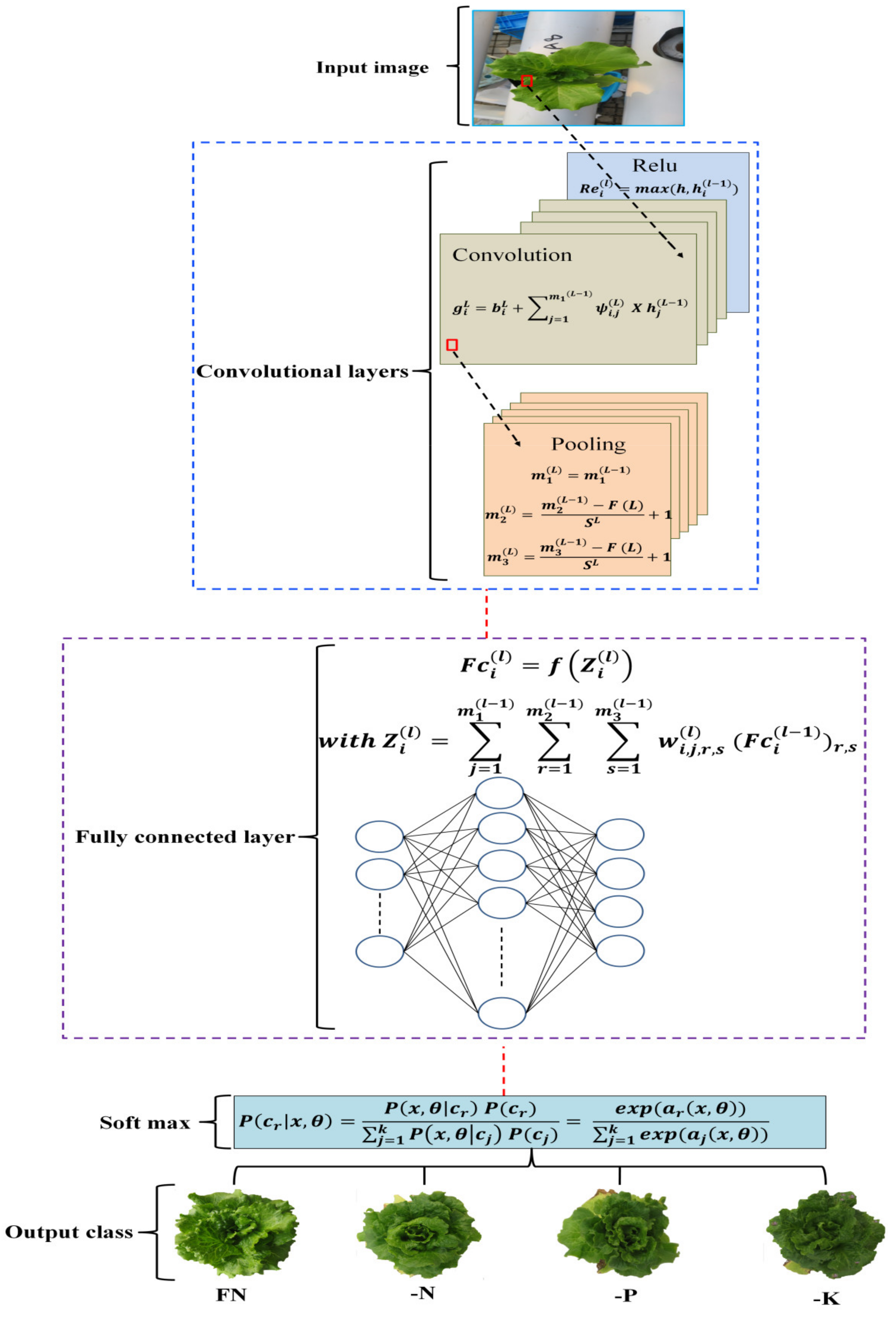
2.9. DCNNs Classifiers
2.10. Performance Evaluation of Segmentation and Classification Methods
2.11. Statistical Analyses
3. Results and Discussion
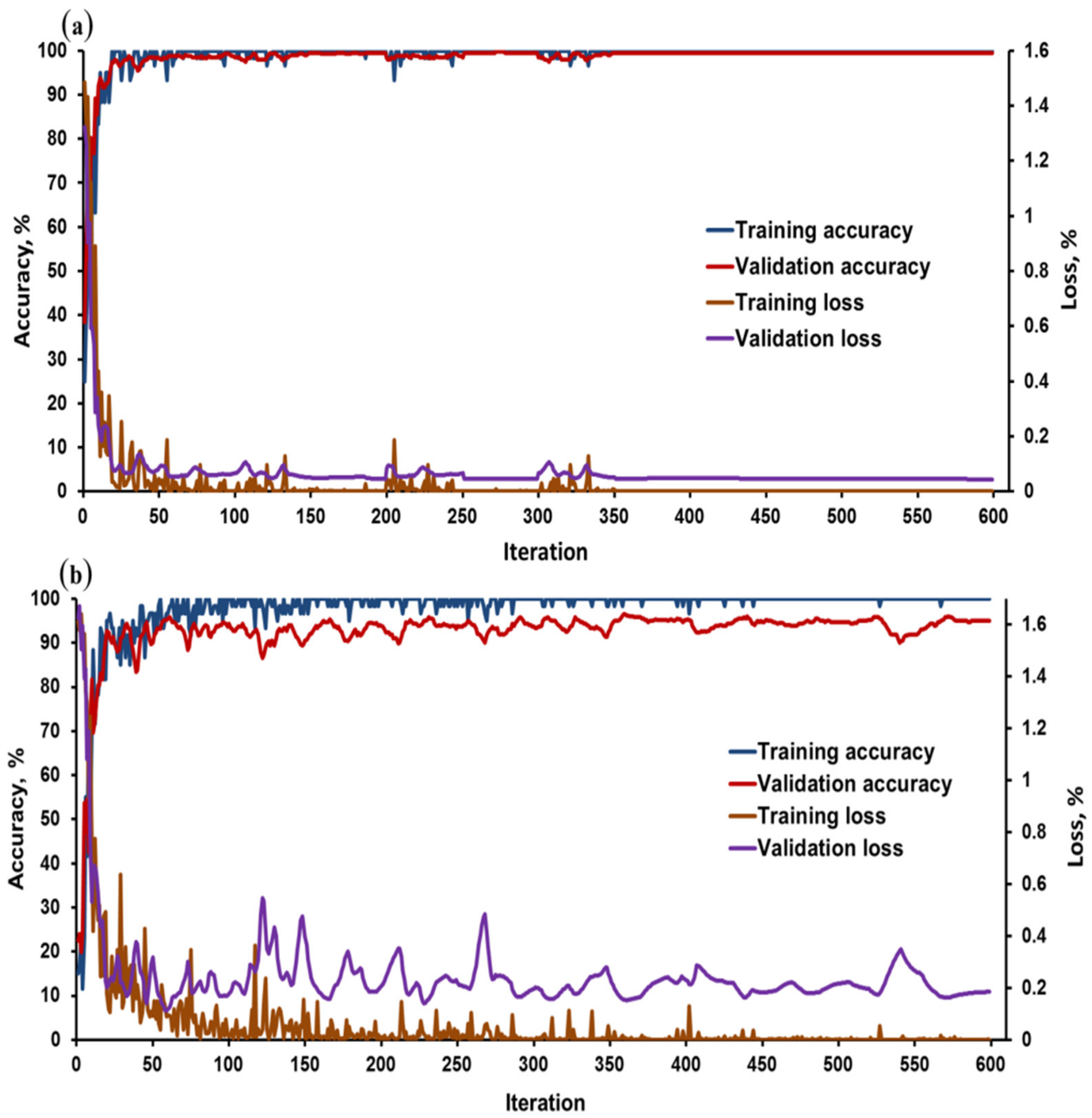
3.1. Training DCNN Models
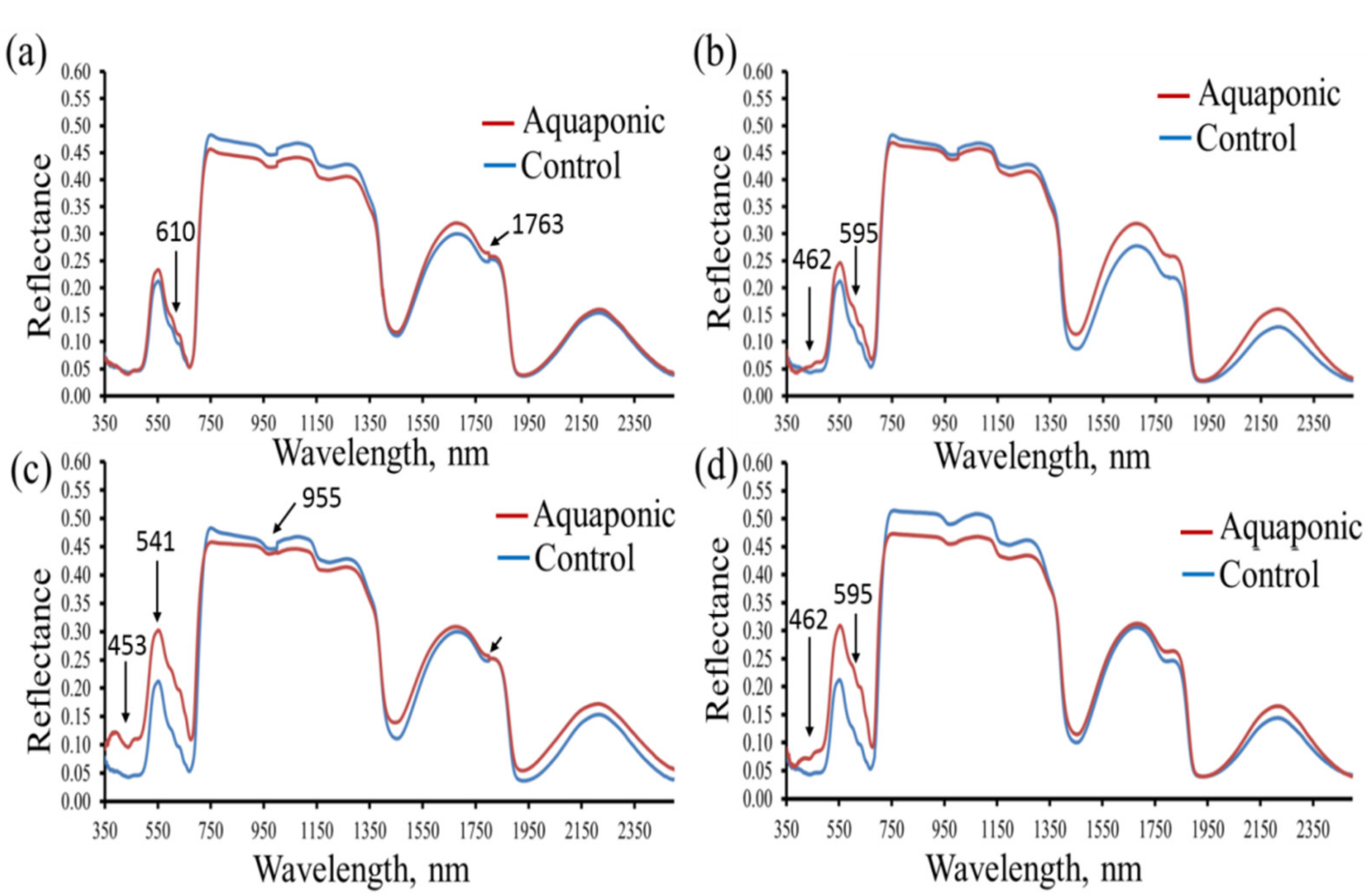
3.2. Changes in Spectral Reflectance under NPK Levels
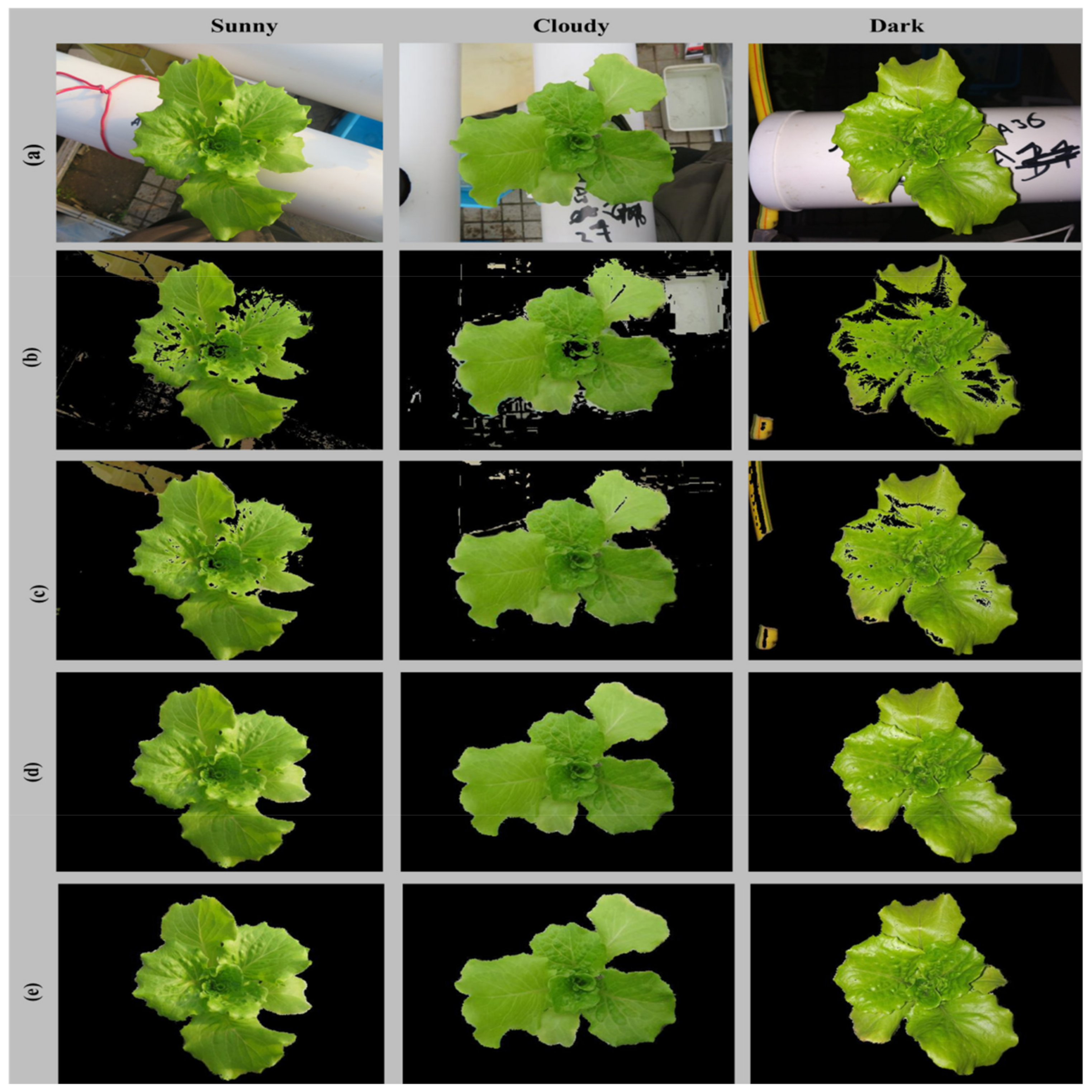
3.3. Evaluation of Segmentation Methods
3.4. Analysis of Variance
3.5. Performance of Classification Methods
4. Conclusions
Author Contributions
Funding
Data Availability Statement
Acknowledgments
Conflicts of Interest
References
- Majid, M.; Khan, J.N.; Shah, Q.M.A.; Masoodi, K.Z.; Afroza, B.; Parvaze, S. Evaluation of hydroponic systems for the cultivation of Lettuce (Lactuca sativa L., var. Longifolia) and comparison with protected soil-based cultivation. Agric. Water Manag. 2021, 245, 106572. [Google Scholar] [CrossRef]
- Yanes, A.R.; Martinez, P.; Ahmad, R.J. Towards automated aquaponics: A review on monitoring, IoT, and smart systems. J. Clean. Prod. 2020, 263, 121571. [Google Scholar] [CrossRef]
- Fischer, H.; Romano, N.; Jones, J.; Howe, J.; Renukdas, N.; Sinha, A.K. Comparing water quality/bacterial composition and productivity of largemouth bass Micropterus salmoides juveniles in a recirculating aquaculture system versus aquaponics as well as plant growth/mineral composition with or without media. Aquaculture 2021, 538, 736554. [Google Scholar] [CrossRef]
- Gao, Y.; Zhang, H.; Peng, C.; Lin, Z.; Li, D.; Lee, C.T.; Wu, W.-M.; Li, C.J. Enhancing nutrient recovery from fish sludge using a modified biological aerated filter with sponge media with extended filtration in aquaponics. J. Clean. Prod. 2021, 320, 128804. [Google Scholar] [CrossRef]
- Yang, T.; Kim, H.J. Characterizing Nutrient Composition and Concentration in Tomato-, Basil-, and Lettuce-Based Aquaponic and Hydroponic Systems. Water 2020, 12, 1259. [Google Scholar] [CrossRef]
- Pineda-Pineda, J.; Miranda-Velázquez, I.; Rodríguez-Pérez, J.; Ramírez-Arias, J.; Pérez-Gómez, E.; García-Antonio, I.; Morales-Parada, J. Nutrimental balance in aquaponic lettuce production. In Proceedings of the International Symposium on New Technologies and Management for Greenhouses-GreenSys. Acta Hortic. 2015, 1170, 1093–1100. [Google Scholar]
- Cook, S.; Bramley, R. Coping with variability in agricultural production-implications for soil testing and fertiliser management. Commun. Soil Sci. Plant Anal. 2000, 31, 1531–1551. [Google Scholar] [CrossRef]
- Xu, Z.; Guo, X.; Zhu, A.; He, X.; Zhao, X.; Han, Y.; Subedi, R. Using Deep Convolutional Neural Networks for Image-Based Diagnosis of Nutrient Deficiencies in Rice. Comput. Intell. Neurosci. 2020, 2020, 7307252. [Google Scholar] [CrossRef]
- Barbedo, J.G.A. Detection of nutrition deficiencies in plants using proximal images and machine learning: A review. Comput. Electron. Agric. 2019, 162, 482–492. [Google Scholar] [CrossRef]
- Gouda, M.; Chen, K.; Li, X.; Liu, Y.; He, Y. Detection of microalgae single-cell antioxidant and electrochemical potentials by gold microelectrode and Raman micro-spectroscopy combined with chemometrics. Sens. Actuators B Chem. 2021, 329, 129229. [Google Scholar] [CrossRef]
- Gouda, M.; El-Din Bekhit, A.; Tang, Y.; Huang, Y.; Huang, L.; He, Y.; Li, X. Recent innovations of ultrasound green technology in herbal phytochemistry: A review. Ultrason. Sonochem. 2021, 73, 105538. [Google Scholar] [CrossRef] [PubMed]
- Eshkabilov, S.; Lee, A.; Sun, X.; Lee, C.W.; Simsek, H. Hyperspectral imaging techniques for rapid detection of nutrient content of hydroponically grown lettuce cultivars. Comput. Electron. Agric. 2021, 181, 105968. [Google Scholar] [CrossRef]
- Li, D.; Li, C.; Yao, Y.; Li, M.; Liu, L. Modern imaging techniques in plant nutrition analysis: A review. Comput. Electron. Agric. 2020, 174, 105459. [Google Scholar] [CrossRef]
- Lisu, C.; Yuanyuan, S.; Ke, W.J. Rapid diagnosis of nitrogen nutrition status in rice based on static scanning and extraction of leaf and sheath characteristics. Int. J. Agric. Biol. Eng. 2017, 10, 158–164. [Google Scholar]
- Zhang, K.; Zhang, A.; Li, C. Nutrient deficiency diagnosis method for rape leaves using color histogram on HSV space. Trans. Chin. Soc. Agric. Eng. 2016, 32, 179–187. [Google Scholar]
- Liu, S.; Li, L.; Gao, W.; Zhang, Y.; Liu, Y.; Wang, S.; Lu, J. Diagnosis of nitrogen status in winter oilseed rape (Brassica napus L.) using in-situ hyperspectral data and unmanned aerial vehicle (UAV) multispectral images. Comput. Electron. Agric. 2018, 151, 185–195. [Google Scholar] [CrossRef]
- Wiwart, M.; Fordoński, G.; Żuk-Gołaszewska, K.; Suchowilska, E. Early diagnostics of macronutrient deficiencies in three legume species by color image analysis. Comput. Electron. Agric. 2009, 65, 125–132. [Google Scholar] [CrossRef]
- Pagola, M.; Ortiz, R.; Irigoyen, I.; Bustince, H.; Barrenechea, E.; Aparicio-Tejo, P.; Lamsfus, C.; Lasa, B. New method to assess barley nitrogen nutrition status based on image colour analysis: Comparison with SPAD-502. Comput. Electron. Agric. 2009, 65, 213–218. [Google Scholar] [CrossRef]
- Story, D.; Kacira, M.; Kubota, C.; Akoglu, A.; An, L. Lettuce calcium deficiency detection with machine vision computed plant features in controlled environments. Comput. Electron. Agric. 2010, 74, 238–243. [Google Scholar] [CrossRef]
- Sanyal, P.; Bhattacharya, U.; Parui, S.K.; Bandyopadhyay, S.K.; Patel, S. Color texture analysis of rice leaves diagnosing deficiency in the balance of mineral levels towards improvement of crop productivity. In Proceedings of the 10th International Conference on Information Technology (ICIT 2007), Rourkela, India, 17–20 December 2007; pp. 85–90. [Google Scholar]
- Hafsi, C.; Falleh, H.; Saada, M.; Ksouri, R.; Abdelly, C. Potassium deficiency alters growth, photosynthetic performance, secondary metabolites content, and related antioxidant capacity in Sulla carnosa grown under moderate salinity. Plant Physiol. Biochem. 2017, 118, 609–617. [Google Scholar] [CrossRef] [PubMed]
- Wang, Z.; Wang, E.; Zhu, Y. Image segmentation evaluation: A survey of methods. Artif. Intell. Rev. 2020, 53, 5637–5674. [Google Scholar] [CrossRef]
- Guo, Y.; Liu, Y.; Georgiou, T.; Lew, M.S. A review of semantic segmentation using deep neural networks. Int. J. Multimed. Inf. Retr. 2018, 7, 87–93. [Google Scholar] [CrossRef] [Green Version]
- Abdalla, A.; Cen, H.; El-manawy, A.; He, Y. Infield oilseed rape images segmentation via improved unsupervised learning models combined with supreme color features. Comput. Electron. Agric. 2019, 162, 1057–1068. [Google Scholar] [CrossRef]
- Zhou, L.; Zhang, C.; Taha, M.F.; Wei, X.; He, Y.; Qiu, Z.; Liu, Y. Wheat Kernel Variety Identification Based on a Large Near-Infrared Spectral Dataset and a Novel Deep Learning-Based Feature Selection Method. Front. Plant Sci. 2020, 11, 575810. [Google Scholar] [CrossRef] [PubMed]
- Ning, F.; Delhomme, D.; LeCun, Y.; Piano, F.; Bottou, L.; Barbano, P.E. Toward automatic phenotyping of developing embryos from videos. IEEE Trans. Image Process. 2005, 14, 1360–1371. [Google Scholar] [CrossRef] [Green Version]
- Lee, S.H.; Chan, C.S.; Wilkin, P.; Remagnino, P. Deep-plant: Plant identification with convolutional neural networks. In Proceedings of the 2015 IEEE International Conference on Image Processing (ICIP), Quebec City, QC, Canada, 27–30 September 2015; pp. 452–456. [Google Scholar]
- Zhou, L.; Zhang, C.; Taha, M.; Qiu, Z.; He, L. Determination of Leaf Water Content with a Portable NIRS System Based on Deep Learning and Information Fusion Analysis. Trans. ASABE 2021, 64, 127–135. [Google Scholar] [CrossRef]
- Sladojevic, S.; Arsenovic, M.; Anderla, A.; Culibrk, D.; Stefanovic, D. Deep neural networks based recognition of plant diseases by leaf image classification. Comput. Intell. Neurosci. 2016, 2016, 3289801. [Google Scholar] [CrossRef] [Green Version]
- Chu, H.; Zhang, C.; Wang, M.; Gouda, M.; Wei, X.; He, Y.; Liu, Y. Hyperspectral imaging with shallow convolutional neural networks (SCNN) predicts the early herbicide stress in wheat cultivars. J. Hazard. Mater. 2021, 421, 126706. [Google Scholar] [CrossRef]
- Badrinarayanan, V.; Kendall, A.; Cipolla, R. Segnet: A deep convolutional encoder-decoder architecture for image segmentation. IEEE Trans. Pattern Anal. Mach. Intell. 2017, 39, 2481–2495. [Google Scholar] [CrossRef]
- Ma, X.; Deng, X.; Qi, L.; Jiang, Y.; Li, H.; Wang, Y.; Xing, X. Fully convolutional network for rice seedling and weed image segmentation at the seedling stage in paddy fields. PLoS ONE 2019, 14, e0215676. [Google Scholar] [CrossRef]
- Zhao, H.; Shi, J.; Qi, X.; Wang, X.; Jia, J. Pyramid scene parsing network. In Proceedings of the IEEE Conference on Computer Vision and Pattern Recognition, Honolulu, HI, USA, 21–26 July 2017; pp. 2881–2890. [Google Scholar]
- Szegedy, C.; Vanhoucke, V.; Ioffe, S.; Shlens, J.; Wojna, Z. Rethinking the inception architecture for computer vision. In Proceedings of the IEEE Conference on Computer Vision and Pattern Recognition, Las Vegas, NV, USA, 27–30 June 2016; pp. 2818–2826. [Google Scholar]
- He, K.; Zhang, X.; Ren, S.; Sun, J. Deep residual learning for image recognition. In Proceedings of the IEEE Conference on Computer Vision and Pattern Recognition, Las Vegas, NV, USA, 27–30 June 2016; pp. 770–778. [Google Scholar]
- Condori, R.H.M.; Romualdo, L.M.; Bruno, O.M.; de Cerqueira Luz, P.H. Comparison between traditional texture methods and deep learning descriptors for detection of nitrogen deficiency in maize crops. In Proceedings of the 2017 Workshop of Computer Vision (WVC), Venice, Italy, 22–27 October 2017; pp. 7–12. [Google Scholar]
- Ghosal, S.; Blystone, D.; Singh, A.K.; Ganapathysubramanian, B.; Singh, A.; Sarkar, S. An explainable deep machine vision framework for plant stress phenotyping. Proc. Natl. Acad. Sci. USA 2018, 115, 4613–4618. [Google Scholar] [CrossRef] [PubMed] [Green Version]
- Tran, T.-T.; Choi, J.-W.; Le, T.-T.H.; Kim, J.W. A comparative study of deep CNN in forecasting and classifying the macronutrient deficiencies on development of tomato plant. Appl. Sci. 2019, 9, 1601. [Google Scholar] [CrossRef] [Green Version]
- Abdalla, A.; Cen, H.; Wan, L.; Mehmood, K.; He, Y. Nutrient Status Diagnosis of Infield Oilseed Rape via Deep Learning-Enabled Dynamic Model. IEEE Trans. Ind. Inform. 2021, 17, 4379–4389. [Google Scholar] [CrossRef]
- Palm, H.W.; Knaus, U.; Appelbaum, S.; Strauch, S.M.; Kotzen, B. Coupled aquaponics systems. In Aquaponics Food Production Systems, 1st ed.; Springer: Cham, Switzerland, 2019; pp. 163–199. [Google Scholar]
- Mao, H.; Gao, H.; Zhang, X.; Kumi, F. Nondestructive measurement of total nitrogen in lettuce by integrating spectroscopy and computer vision. Sci. Hortic. 2015, 184, 1–7. [Google Scholar] [CrossRef]
- Lan, W.; Wu, A.; Wang, Y.; Wang, J.; Li, J. Ionic solidification and size effect of hemihydrate phosphogypsum backfill. China Environ. Sci. 2019, 39, 210–218. [Google Scholar]
- Tian, X.; YanYan, W.; LaiHao, L.; WanLing, L.; XianQing, Y.; Xiao, H.; ShaoLing, Y. Material characteristics and eating quality of Trachinotus ovatus muscle. Shipin Kexue Food Sci. 2019, 40, 104–112. [Google Scholar]
- Somerville, C.; Cohen, M.; Pantanella, E.; Stankus, A.; Lovatelli, A. Small-Scale Aquaponic Food Production: Integrated Fish and Plant Farming; FAO Fisheries and Aquaculture Technical Paper; FAO: Rome, Italy, 2014; p. 1. [Google Scholar]
- Van Delden, S.H.; Nazarideljou, M.J.; Marcelis, L.F. Nutrient solutions for Arabidopsis thaliana: A study on nutrient solution composition in hydroponics systems. Plant Methods 2020, 16, 72. [Google Scholar] [CrossRef]
- Chen, Z.; Wang, X.J.C.; Systems, I.L. Model for estimation of total nitrogen content in sandalwood leaves based on nonlinear mixed effects and dummy variables using multispectral images. Chemom. Intell. Lab. Syst. 2019, 195, 103874. [Google Scholar] [CrossRef]
- Liu, N.; Townsend, P.A.; Naber, M.R.; Bethke, P.C.; Hills, W.B.; Wang, Y. Hyperspectral imagery to monitor crop nutrient status within and across growing seasons. Remote Sens. Environ. 2021, 255, 112303. [Google Scholar] [CrossRef]
- Pacumbaba, R., Jr.; Beyl, C. Changes in hyperspectral reflectance signatures of lettuce leaves in response to macronutrient deficiencies. Adv. Space Res. 2011, 48, 32–42. [Google Scholar] [CrossRef]
- Van Eysinga, J.R.; Smilde, K.W. Nutritional Disorders in Glasshouse Tomatoes, Cucumbers and Lettuce, 1st ed.; Centre for Agricultural Publishing and Documentation of Wageningen University: Gelderland, The Netherlands, 1981. [Google Scholar]
- Ben Chaabane, S.; Sayadi, M.; Fnaiech, F.; Brassart, E. Colour image segmentation using homogeneity method and data fusion techniques. EURASIP J. Adv. Signal Process. 2009, 2010, 367297. [Google Scholar] [CrossRef] [Green Version]
- Khan, M.W. A survey: Image segmentation techniques. Int. J. Future Comput. Commun. 2014, 3, 89. [Google Scholar] [CrossRef] [Green Version]
- Corrias, G.; Micheletti, G.; Barberini, L.; Suri, J.S.; Saba, L. Texture analysis imaging “what a clinical radiologist needs to know”. Eur. J. Radiol. 2022, 146, 110055. [Google Scholar] [CrossRef] [PubMed]
- Kociołek, M.; Strzelecki, M.; Obuchowicz, R. Does image normalization and intensity resolution impact texture classification? Comput. Med. Imaging Graph. 2020, 81, 101716. [Google Scholar] [CrossRef]
- Kebapci, H.; Yanikoglu, B.; Unal, G. Plant image retrieval using color, shape and texture features. Comput. J. 2011, 54, 1475–1490. [Google Scholar] [CrossRef] [Green Version]
- Azimi, S.; Kaur, T.; Gandhi, T.K. A deep learning approach to measure stress level in plants due to Nitrogen deficiency. Measurement 2020, 173, 108650. [Google Scholar] [CrossRef]
- Breiman, L.; Friedman, J.H.; Olshen, R.A.; Stone, C.J. Classification and Regression Trees; Routledge: Abingdon, UK, 2017. [Google Scholar]
- Agarwal, M.; Gupta, S.K.; Biswas, K. Development of Efficient CNN model for Tomato crop disease identification. Sustain. Comput. Inform. Syst. 2020, 28, 100407. [Google Scholar] [CrossRef]
- Atila, Ü.; Uçar, M.; Akyol, K.; Uçar, E. Plant leaf disease classification using EfficientNet deep learning model. Ecol. Inform. 2021, 61, 101182. [Google Scholar] [CrossRef]
- Pan, S.J.; Yang, Q. A survey on transfer learning. IEEE Trans. Knowl. Data Eng. 2009, 22, 1345–1359. [Google Scholar] [CrossRef]
- Mohanty, S.P.; Hughes, D.P.; Salathé, M. Using deep learning for image-based plant disease detection. Front. Plant Sci. 2016, 7, 1419. [Google Scholar] [CrossRef] [Green Version]
- Mani, B.; Shanmugam, J. Estimating plant macronutrients using VNIR spectroradiometry. Pol. J. Environ. Stud. 2019, 28, 1831–1837. [Google Scholar] [CrossRef]
- Sridevy, S.; Vijendran, A.S.; Jagadeeswaran, R.; Djanaguiraman, M. Nitrogen and potassium deficiency identification in maize by image mining, spectral and true colour response. Indian J. Plant Physiol. 2018, 23, 91–99. [Google Scholar] [CrossRef]
- Siedliska, A.; Baranowski, P.; Pastuszka-Woźniak, J.; Zubik, M.; Krzyszczak, J. Identification of plant leaf phosphorus content at different growth stages based on hyperspectral reflectance. BMC Plant Biol. 2021, 21, 28. [Google Scholar] [CrossRef] [PubMed]
- Abdalla, A.; Cen, H.; Wan, L.; Rashid, R.; Weng, H.; Zhou, W.; He, Y. Fine-tuning convolutional neural network with transfer learning for semantic segmentation of ground-level oilseed rape images in a field with high weed pressure. Comput. Electron. Agric. 2019, 167, 105091. [Google Scholar] [CrossRef]
- Phonsa, G.; Manu, K. A survey: Image segmentation techniques. In Harmony Search and Nature Inspired Optimization Algorithms; Springer: Cham, Switzerland; pp. 1123–1140. 2019. [Google Scholar]
- Gouda, M.; Ma, M.; Sheng, L.; Xiang, X. SPME-GC-MS & metal oxide E-Nose 18 sensors to validate the possible interactions between bio-active terpenes and egg yolk volatiles. Food Res. Int. 2019, 125, 108611. [Google Scholar] [PubMed]
- Yilmaz, A.; Demircali, A.A.; Kocaman, S.; Uvet, H. Comparison of Deep Learning and Traditional Machine Learning Techniques for Classification of Pap Smear Images. arXiv 2009, arXiv:2009.06366. [Google Scholar]
- Bosilj, P.; Aptoula, E.; Duckett, T.; Cielniak, G. Transfer learning between crop types for semantic segmentation of crops versus weeds in precision agriculture. J. Field Robot. 2020, 37, 7–19. [Google Scholar] [CrossRef]
- Manickam, R.; Rajan, S.K.; Subramanian, C.; Xavi, A.; Eanoch, G.J.; Yesudhas, H.R. Person identification with aerial imaginary using SegNet based semantic segmentation. Earth Sci. Inform. 2020, 13, 1293–1304. [Google Scholar] [CrossRef]
- Li, Y.; Shi, T.; Zhang, Y.; Chen, W.; Wang, Z.; Li, H. Learning deep semantic segmentation network under multiple weakly-supervised constraints for cross-domain remote sensing image semantic segmentation. ISPRS J. Photogramm. Remote Sens. 2021, 175, 20–33. [Google Scholar] [CrossRef]
- Benjdira, B.; Bazi, Y.; Koubaa, A.; Ouni, K. Unsupervised domain adaptation using generative adversarial networks for semantic segmentation of aerial images. Remote Sens. 2019, 11, 1369. [Google Scholar] [CrossRef] [Green Version]
- Chantharaj, S.; Pornratthanapong, K.; Chitsinpchayakun, P.; Panboonyuen, T.; Vateekul, P.; Lawavirojwong, S.; Srestasathiern, P.; Jitkajornwanich, K. Semantic segmentation on medium-resolution satellite images using deep convolutional networks with remote sensing derived indices. In Proceedings of the 2018 15th International Joint Conference on Computer Science and Software Engineering (JCSSE), Nakhon Pathom, Thailand, 11–13 July 2018; pp. 1–6. [Google Scholar]
- Chen, L.; Lin, L.; Cai, G.; Sun, Y.; Huang, T.; Wang, K.; Deng, J. Identification of nitrogen, phosphorus, and potassium deficiencies in rice based on static scanning technology and hierarchical identification method. PLoS ONE 2014, 9, e113200. [Google Scholar]
- Lee, J.-H.; Kim, D.-H.; Jeong, S.-N.; Choi, S.-H. Detection and diagnosis of dental caries using a deep learning-based convolutional neural network algorithm. J. Dent. 2018, 77, 106–111. [Google Scholar] [CrossRef]
- Sajedi, H.; Mohammadipanah, F.; Pashaei, A. Automated identification of Myxobacterial genera using convolutional neural network. Sci. Rep. 2019, 9, 18238. [Google Scholar] [CrossRef] [PubMed] [Green Version]
- Amri, A.; A’Fifah, I.; Ismail, A.R.; Zarir, A.A. Comparative performance of deep learning and machine learning algorithms on imbalanced handwritten data. Int. J. Adv. Comput. Sci. Appl. 2018, 9, 258–264. [Google Scholar]


| Day | Leaf Content of Nutrients, g/kg DW | |||||
|---|---|---|---|---|---|---|
| Aquaponic | Hydroponic (Control), FN | |||||
| N | P | K | N | P | K | |
| 15 | 3.01 | 0.21 | 3.05 | 6.05 | 0.75 | 6.01 |
| 20 | 3.5 | 0.55 | 3.4 | 6.35 | 0.74 | 6.32 |
| 25 | 3.54 | 0.34 | 3.7 | 5.57 | 0.67 | 6.52 |
| 30 | 3.2 | 0.41 | 4.01 | 5.8 | 0.53 | 6.65 |
| 35 | 2.85 | 0.35 | 4.21 | 5.7 | 0.52 | 6.04 |
| 40 | 4.05 | 0.38 | 2.5 | 6.55 | 0.65 | 6.18 |
| 45 | 3.64 | 0.47 | 3.37 | 5.44 | 0.45 | 6.27 |
| 50 | 2.95 | 0.51 | 3.7 | 5.28 | 0.63 | 6.3 |
| 55 | 4.25 | 0.21 | 3.97 | 5.31 | 0.52 | 6.57 |
| 60 | 2.94 | 0.22 | 4.04 | 5.74 | 0.61 | 6.19 |
| Nutrient | Concentration (mg/L) | |
|---|---|---|
| Aquaponic (Measured) | Control (Optimal) | |
| Total N | 30.8 | 321 |
| P | 10.6 | 36.9 |
| K | 60.8 | 340 |
| Class | Typical Symptoms | Images |
|---|---|---|
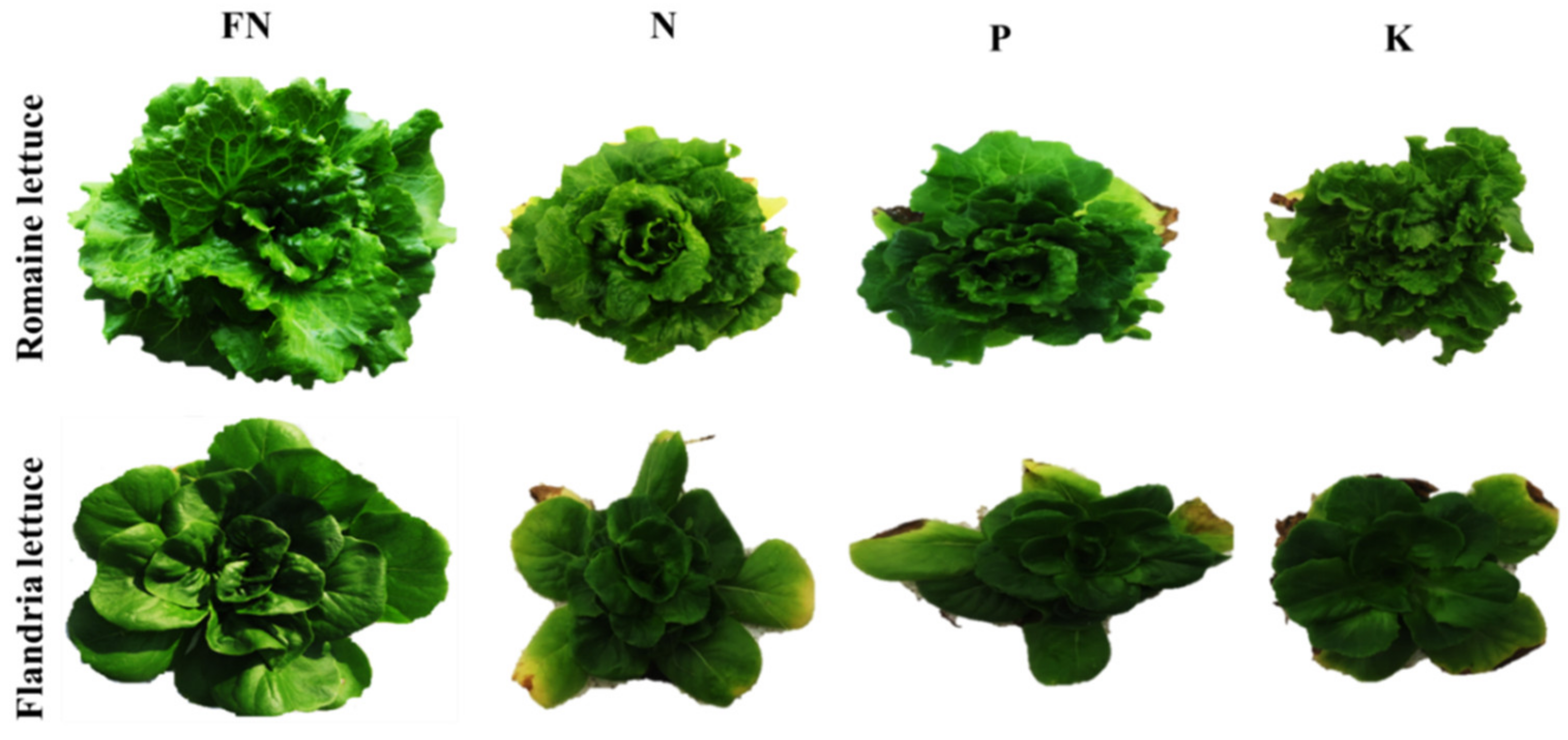
| FN | Healthy plant, leaves are green, and generally with no mottling or spots | 600 |
| -N | Growth is restricted, foliage yellowish green, severe chlorosis of older leaves, and decay of older leaves. | 850 |
| -P | Plants are stunted, older leaves die with severe deficiency, leaf margins of older leaves exhibited chlorotic regions followed by necrotic spots, and leaves are darker than normal. | 550 |
| -K | Growth is reduced, leaves are less crinkled and darker green than normal, with severe deficiency they become more petiolate, necrotic spots on margins of old leaves, and chlorotic spots develop at the tips of older leaves. | 1000 |
| Model | Training Accuracy (%) | Validation Accuracy (%) | Training Time (min) |
|---|---|---|---|
| SegNet | 98.30% | 99.29% | 194 |
| Inceptionv3 | 98.90% | 98.00% | 65 |
| ResNet18 | 97.70% | 92.50% | 87 |
| Model | Acc (%) | Pr (%) | Re (%) | F1_score (%) | Dice Score (%) | ST (s/Image) |
|---|---|---|---|---|---|---|
| SegNet | 99.1 | 99.3 | 99.5 | 99.4 | 99.5 | 0.605 |
| K-means | 83.1 | 83.5 | 83.7 | 83.5 | 83.3 | 5 |
| Thresholding | 75.2 | 75.5 | 75.6 | 75.5 | 75.5 | 0.7 |
| FN | -N | -P | -K | |
|---|---|---|---|---|
| Contrast | 0.314 a | 0.108 b | 0.051 d | 0.074 c |
| Correlation | 0.966 a | 0.658 b | 0.662 c | 0.646 d |
| Energy | 0.962 d | 0.967 c | 0.978 a | 0.974 b |
| Homogeneity | 0.991 d | 0.992 c | 0.995 a | 0.994 b |
| Entropy | 0.928 a | 0.550 b | 0.352 c | 0.431 d |
| Red | 0.835 a | 0.357 b | 0.338 c | 0.340 c |
| Green | 0.782 a | 0.401 b | 0.393 c | 0.392 c |
| Blue | 0.883 a | 0.242 b | 0.269 c | 0.268 c |
| Hue | 0.595 a | 0.064 b | 0.039 c | 0.019 d |
| Saturation | 0.663 a | 0.208 b | 0.093 c | 0.035 d |
| Value | 0.423 a | 0.115 b | 0.038 c | 0.006 d |
| Area | 3762 a | 3652 a | 2035 b | 2636 c |
| Perimeter | 3024 a | 2870 a | 1690 b | 2170 c |
| Convex hull | 92,483 a | 63,213 b | 32,385 c | 47,986 c |
| Predicted Class | Acc (%) | |||||||
|---|---|---|---|---|---|---|---|---|
| FN | -N | -P | -K | Total | ||||
| Incepionv3 | True class | FN | 120 | 0 | 0 | 0 | 120 | 96.5 |
| -N | 1 | 165 | 3 | 1 | 170 | |||
| -P | 2 | 3 | 100 | 5 | 110 | |||
| -K | 0 | 3 | 3 | 194 | 200 | |||
| Total | 123 | 171 | 106 | 200 | 600 | |||
| ResNet18 | True class | FN | 120 | 0 | 0 | 0 | 120 | 92.1 |
| -N | 3 | 150 | 10 | 7 | 170 | |||
| -P | 2 | 7 | 95 | 6 | 110 | |||
| -K | 2 | 4 | 6 | 188 | 200 | |||
| Total | 127 | 161 | 111 | 201 | 600 | |||
| SVM | True class | FN | 110 | 2 | 3 | 5 | 120 | 86.1 |
| -N | 8 | 140 | 12 | 10 | 170 | |||
| -P | 5 | 9 | 88 | 8 | 110 | |||
| -K | 8 | 6 | 7 | 179 | 200 | |||
| Total | 131 | 157 | 110 | 202 | 600 | |||
| KNN | True class | FN | 108 | 2 | 5 | 5 | 120 | 84.5 |
| -N | 8 | 139 | 12 | 11 | 170 | |||
| -P | 5 | 12 | 85 | 8 | 110 | |||
| -K | 10 | 5 | 10 | 175 | 200 | |||
| Total | 131 | 158 | 112 | 199 | 600 | |||
| DT | True class | FN | 100 | 3 | 7 | 10 | 120 | 79.8 |
| -N | 9 | 130 | 15 | 16 | 170 | |||
| -P | 6 | 13 | 80 | 11 | 110 | |||
| -K | 11 | 8 | 12 | 169 | 200 | |||
| Total | 126 | 154 | 114 | 206 | 600 | |||
| Measure | Inceptionv3 | ResNet18 | SVM | KNN | DT |
|---|---|---|---|---|---|
| Acc (%) | 96.5 | 92.1 | 86.1 | 84.5 | 79.8 |
| Pr (%) | 95.7 | 91.6 | 85.5 | 83.7 | 78.9 |
| Re (%) | 96.2 | 92.1 | 85.8 | 84.1 | 79.2 |
| F1_score (%) | 95.9 | 91.8 | 85.6 | 83.8 | 79.0 |
| CT (s/image) | 0.6 | 0.8 | 0.2 | 0.4 | 0.5 |
Publisher’s Note: MDPI stays neutral with regard to jurisdictional claims in published maps and institutional affiliations. |
© 2022 by the authors. Licensee MDPI, Basel, Switzerland. This article is an open access article distributed under the terms and conditions of the Creative Commons Attribution (CC BY) license (https://creativecommons.org/licenses/by/4.0/).
Share and Cite
Taha, M.F.; Abdalla, A.; ElMasry, G.; Gouda, M.; Zhou, L.; Zhao, N.; Liang, N.; Niu, Z.; Hassanein, A.; Al-Rejaie, S.; et al. Using Deep Convolutional Neural Network for Image-Based Diagnosis of Nutrient Deficiencies in Plants Grown in Aquaponics. Chemosensors 2022, 10, 45. https://doi.org/10.3390/chemosensors10020045
Taha MF, Abdalla A, ElMasry G, Gouda M, Zhou L, Zhao N, Liang N, Niu Z, Hassanein A, Al-Rejaie S, et al. Using Deep Convolutional Neural Network for Image-Based Diagnosis of Nutrient Deficiencies in Plants Grown in Aquaponics. Chemosensors. 2022; 10(2):45. https://doi.org/10.3390/chemosensors10020045
Chicago/Turabian StyleTaha, Mohamed Farag, Alwaseela Abdalla, Gamal ElMasry, Mostafa Gouda, Lei Zhou, Nan Zhao, Ning Liang, Ziang Niu, Amro Hassanein, Salim Al-Rejaie, and et al. 2022. "Using Deep Convolutional Neural Network for Image-Based Diagnosis of Nutrient Deficiencies in Plants Grown in Aquaponics" Chemosensors 10, no. 2: 45. https://doi.org/10.3390/chemosensors10020045