
Bridge Condition Deterioration Prediction Using the Whale Optimization Algorithm and Extreme Learning Machine

1
State Key Laboratory of Mountain Bridge and Tunnel Engineering, Chongqing Jiaotong University, Chongqing 400074, China
2
College of Engineering and Technology, Southwest University, Chongqing 400715, China
3
Chongqing Yuhe Expressway Co., Ltd., Chongqing 400799, China
4
Guangxi Nanbai Expressway Co., Ltd., Nanning 530029, China
*
Authors to whom correspondence should be addressed.
Buildings 2023, 13(11), 2730; https://doi.org/10.3390/buildings13112730
Submission received: 2 September 2023
/
Revised: 21 October 2023
/
Accepted: 26 October 2023
/
Published: 29 October 2023
(This article belongs to the Topic Condition Perception and Performance Evaluation of Engineering Structures)
Abstract
:To address the problem in model computations and the limited accuracy of current bridge deterioration prediction methods, this paper proposes a novel bridge deterioration prediction meth-od using the whale optimization algorithm and extreme learning machine (WOA-ELM). First, we collected a dataset consisting of 539 sets of bridge inspection data and determined the necessary influencing factors through correlation analysis. Subsequently, the WOA-ELM algorithm was applied to establish a nonlinear mapping relationship between each influencing factor and the bridge condition indicators. Furthermore, the extreme learning machine (ELM), back-propagation neural network (BPNN), decision trees (DT), and support vector machine (SVM) were employed for comparison to validate the superiority of the proposed method. In addition, this paper provides further substantiation of the model’s exceptional predictive capabilities across diverse bridge components. The results demonstrate the accurate predictive capability of the proposed method for bridge conditions. Compared with ELM, BPNN, DT, and SVM, the proposed method exhibits significant improvements in predictive accuracy, i.e., the correlation coefficient is increased by 4.1%, 11.4%, 24.5%, and 33.6%, and the root mean square error is reduced by 7.3%, 18.0%, 14.8%, and 18.1%, respectively. Moreover, the proposed method presents considerably enhanced generalization capabilities, resulting in the reduction in mean relative error by 11.6%, 15.3%, 6%, and 16.2%. The proposed method presents a robust framework for proactive bridge maintenance.
1. Introduction
The number of highway bridges in China exceeded 960,000 in 2023. With the passage of time, these bridge structures inevitably experience performance degradation, caused by the coupled effects of external service environment factors and internal material deterioration [1,2,3]. Accurately predicting bridge performance evolution holds great theoretical and practical importance for scientific maintenance and extending structural service life [4,5,6].
Extensive research has been conducted by a considerable number of scholars on the establishment of bridge condition prediction models, which are broadly categorized into deterministic and probabilistic models [7]. The former category assumes a fixed and deterministic degradation trend for bridge condition, and utilizes historical periodic inspection data to perform regression fitting of predefined deterioration decay equations. Through this process, the degradation rate of bridge performance under different conditions is estimated. For instance, Yang et al. [8] employed detection data from 398 reinforced concrete bridges to fit a bridge condition degradation model that reveals the changing characteristics of bridge performance during different operational phases. Similarly, Sahar et al. [9] established a degradation regression model for the superstructure of bridges based on extensive bridge inspection data. Subsequently, the model considered eight influencing factors, including service time, span, and traffic volume, and the researchers also conducted sensitivity analysis on these factors. While deterministic models are relatively straightforward to construct, they can be adjusted and updated for different bridges. However, they still struggle to account for the stochastic nature of bridge degradation and demand high-quality historical inspection data. In contrast, the second type of model considers the degradation rate as a random variable and utilizes the theory of stochastic processes to simulate the deteriorating trends of bridge structural conditions. Moreover, most probability models have implemented Markov processes [7]. For example, Zhang et al. [10] used five years of continuous bridge inspection data from 445 hollow slab bridges and developed a bridge condition degradation prediction model based on a multi-stage Markov chain. Furthermore, their findings revealed that the state transition probability matrix in the model closely matched actual conditions. Additionally, Wellalage et al. [11] proposed a Metropolis–Hastings optimized Markov chain Monte Carlo method to calculate the state transition matrix of the typical components of railway bridges. Moreover, they compared it with regression and Bayesian models to demonstrate its superiority. In addition, Thanh et al. [12] addressed data insufficiency issues in Markov processes by incorporating a physical-empirical model. The results indicated that the model could derive the state transition matrix using the least squares method. Nevertheless, probabilistic models remain dependent on subjective engineering judgments and necessitate ongoing updates, constraining their potential for further optimization to ensure predictive efficacy.
In recent years, owing to the rapid development and extensive application of machine learning, various scholars have started adopting the extreme learning machine (ELM) model to enhance the predictive performance of models. For instance, Jiang et al. [13] utilized the ELM model to indirectly predict the remaining lifespan of lithium batteries, achieving an error control within 5%. Furthermore, He et al. [14] demonstrated that the ELM model could achieve a 94.44% accuracy in circuit fault prediction in just one millisecond, highlighting the significant advantages of ELM in predictive performance. Subsequently, researchers discovered that optimizing the initial weights and thresholds could further improve ELM’s predictive capabilities.
The whale optimization algorithm (WOA) is a novel swarm intelligence and bio-inspired optimization algorithm proposed by Mirjalili et al. [15] in 2016. It draws inspiration from the hunting behavior of humpback whales and simulates their unique spiral bubble-net hunting strategy, aiming to achieve optimization for complex problems. Additionally, WOA incorporates three independent population update mechanisms: search for prey, encircling prey, and spiral update. Effectively, WOA eliminates the need for manually setting various control parameter values. Consequently, this approach significantly enhances algorithm efficiency and reduces application complexity. In this context, Lu et al. [16] established a microgrid fault analysis model using the whale optimization algorithm-enhanced extreme learning machine (WOA-ELM). When compared to the backpropagation neural network (BPNN), radial basis function neural network, and conventional ELM, WOA-ELM demonstrated faster learning speed, stronger generalization capability, and higher recognition accuracy. Similarly, Li et al. [17] conducted experiments comparing various optimization algorithms for ELM prediction models, and their findings revealed that WOA-ELM outperformed ELM, genetic algorithm-optimized ELM, cuckoo search-optimized ELM, and dandelion algorithm-optimized ELM in terms of predictive performance. Certainly, there are many other effective metaheuristic algorithms. For instance, Nadimi-Shahraki et al. [18] analyzed the performance of the MTDE algorithm based on the multi-trial vector-based differential evolution method for problems such as the pressure vessel, welded beam, tension/compression spring, and three-bar truss. Their analysis demonstrated that the MTDE algorithm exhibits improved performance and high precision in finding the optimal solution. Liu et al. [19] conducted research on the agricultural drone route-planning problem using the grey wolf optimization algorithm. They discovered that this algorithm can effectively generate drone trajectories that meet agricultural operational requirements, and exhibits improved performance and high precision in finding optimal solutions.
Considering the high data quality requirements, limited applicability, and the subjective influence on model updates in existing methods, this paper proposes a bridge deterioration prediction model based on WOA-ELM. To enhance the model’s applicability beyond a single bridge, the study utilizes a dataset comprising 539 sets of diverse bridge inspection data. It establishes nonlinear mapping relationships between 11 influencing factors, including time, bridge type, span, and others, and the indicators representing the bridge’s condition. By comparing the results of this paper’s approach with various machine learning prediction models, its superiority is confirmed.
2. Extreme Learning Machine
The ELM [20,21,22] is a machine learning algorithm based on the construction of a feedforward neural network. Its fundamental principle involves randomly generating connection weights between the input layer and the hidden layer, as well as thresholds for the hidden layer nodes, and then obtaining the optimal solution through straightforward matrix computations. Compared to traditional feedforward neural network algorithms, ELM exhibits strong learning capabilities, superior generalization performance, and simplicity in parameter configuration. The network structure of ELM is illustrated in Figure 1.
In consideration of the single-hidden-layer ELM network architecture illustrated in Figure 1, we assume the existence of n arbitrary samples (Xi, Yi). In this context, represents the input matrix, and signifies the output matrix. The input layer of the ELM comprises n nodes, while the hidden layer consists of l nodes, and the output layer encompasses m nodes. The mathematical representation of the ELM can be succinctly articulated as follows:
In this equation, the symbol signifies the input weight matrix, while represents the output weight matrix. Additionally, the notations and are employed to denote the activation function and bias of the hidden layer neurons correspondingly.
The primary objective of learning in a single-hidden-layer neural network is to minimize the output error. This objective necessitates identifying distinctive values for , , and that satisfy the requirements in Equation (2). Consequently, these values can be succinctly represented using matrices as follows:
In this expression, represents the output weight matrix, and corresponds to the desired output matrix.
The learning process of ELM can be approximated as solving a nonlinear optimization problem. When the activation function is infinitely differentiable, the input weights and biases of ELM are stochastically determined. Simultaneously, the output matrix of the hidden layer becomes uniquely determined throughout the training process. Consequently, the ELM learning process is analogous to finding the least squares solution, which can be mathematically expressed as follows:
In this equation, stands for the Moore–Penrose pseudoinverse of the hidden layer output matrix.
3. Optimization of the WOA Algorithm
Given the unknown nature of the optimal initial weights and thresholds for ELM, the present study employs WOA for optimization. By considering the optimal position of an individual within the initial whale population as the best candidate set for the target position, two essential steps are achieved. Firstly, the optimal individual’s position serves as a reference for identifying the best candidate set. Secondly, the remaining individuals progressively converge towards this identified best candidate set, while iterative position updates are conducted to iteratively approach the optimal solution [23]. The mathematical expression for this stage is presented below:
In this equation, X(t + 1) represents the position vector of the individual whale after iterative updates at the current iteration. X(t) denotes the position vector of the individual whale at the current iteration. X*(t) signifies the position vector of the optimal individual within the current whale population. D stands for the random distance vector between the whale and the target. A and C are coefficient vectors. a represents the linearly decreasing attenuation coefficient of . r is a random value between 0 and 1. t represents the current iteration number, and T denotes the maximum number of iterations.
During each iteration update, a random individual whale is selected, and the distance between this whale and the target is calculated. Subsequently, a spiral equation is established between the individual whale and the target based on this distance calculation. The mathematical expression for this spiral equation is as follows:
In the provided equation, represents the distance vector between the current individual whale and the target. The constant b defines the logarithmic spiral curve, and l is a random variable between 0 and 1.
In this study, a probability threshold p is set to simultaneously achieve both of the aforementioned approaches. This ensures that the sperm whale randomly selects either of the two models with equal probabilities. The final mathematical expression for this stage is presented below:
In this equation, p is a random variable between −1 and 1.
To enhance the search capability further, this study calculates the magnitude of A in real time during each iteration. When is below the threshold 1, the selection of the optimal individual from the whale population as the target for position updates, in accordance with Equation (7), exemplifies the algorithm’s local search capability. Additionally, when the magnitude of surpasses a specific threshold of 1, the algorithm enhances its global search capability. This enhancement is achieved by adopting a strategy that involves randomly selecting a whale individual as the target position and updating the positions of other individuals accordingly. The mathematical expression for this process is provided below:
In this formula, the symbol represents the position vector of a randomly selected whale individual from the current whale population.
4. Bridge Condition Deterioration Prediction Model Based on WOA-ELM
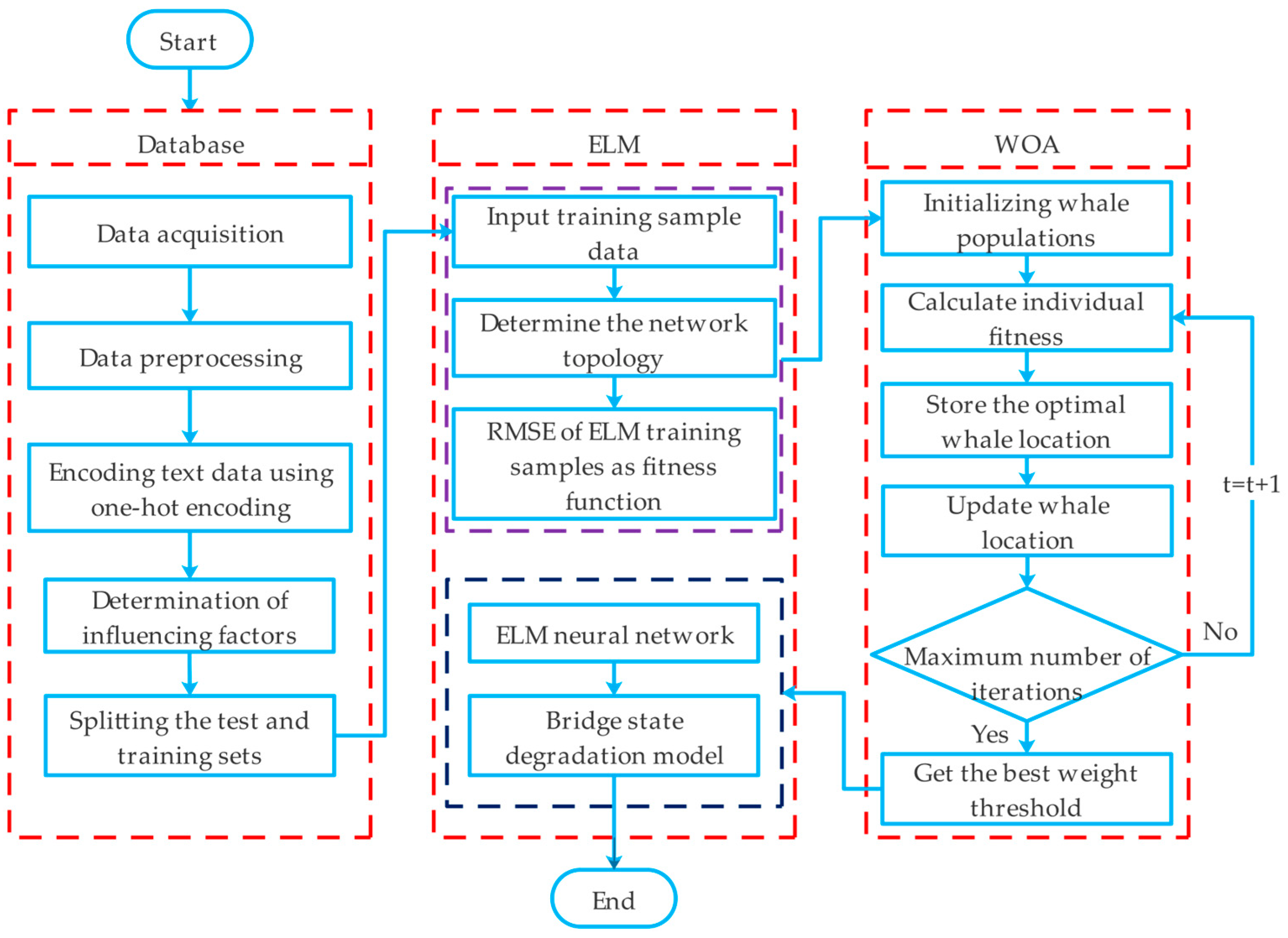
The objective of this study is to establish a data-centric bridge health prediction model. In this context, a substantial amount of bridge inspection data are utilized within this study. However, the ELM model’s initial weights and thresholds exhibit randomness and lack of consistency, thereby constraining the further enhancement of model accuracy. To address this challenge, WOA is introduced as a remedy. The initial phase entails data preprocessing. During this phase, 539 sets of bridge inspection data are organized into a dataset to facilitate training and testing with WOA-ELM. The subsequent phase involves leveraging the training set to calculate optimal hyperparameters for the ELM predictive model and establish the network topology. Following that, WOA is applied, utilizing the training set and network topology, to compute the most suitable model weights for this dataset. In the ultimate phase, optimized initial weights and thresholds are incorporated into the ELM model for training, culminating in the development of a bridge deterioration prediction model. Figure 2 illustrates the workflow of the regional bridge deterioration prediction model based on WOA-ELM.
5. Performance Metrics for Evaluation
To assess the performance of the model, this study employs the mean absolute error (MAE), mean relative error (MRE), root mean square error (RMSE), and correlation coefficient (R) as evaluation metrics for the predictive model [24,25]. The computations for each performance evaluation metric are as follows:
where MAE measures the absolute deviation between the predicted values and the expected values. It effectively addresses the issue of error cancellation and serves as an indicator of the model’s generalization capability. MRE measures the relative deviation between the predicted and expected values, providing valuable insights into the model’s generalization ability. RMSE assesses the fluctuations in deviation between the predicted and expected values, thus serving as a reflection of the model’s accuracy. R signifies the goodness of fit and predictive accuracy of the model. Here, denotes the actual value of the ith sample, and represents the model’s predicted value for the same sample. The variable N corresponds to the total number of samples, and < 0.4 denotes a low-degree linear correlation. A correlation coefficient value within the range 0.4 < < 0.7 indicates a moderate correlation, whereas a value within the range 0.7 < < 1 signifies a high-degree linear correlation.
6. Method Validation
6.1. Dataset
Establishing a comprehensive bridge condition database serves as an essential foundation for investigating the evolutionary patterns of bridge deterioration. This article gathers documentary materials, including sets of periodic inspection reports, construction design drawings, repair drawings, and maintenance records, for 539 urban bridges situated from 2011 to 2019.
6.1.1. Data Preprocessing
When dealing with multi-source data, a key-value pair collection approach is employed to represent and store each individual bridge entity. The former specifies the specific features, while the latter assigns corresponding data to these features [26]. Bridge entity attributes should encompass information from three aspects: the route level, bridge level, and component level. Different attributes have varying data formats, such as text-based or numerical data. Text-based data typically represent the name or label of the subject under study, while numerical data indicate quantitative relationships between data points.
However, the integrated raw database cannot be directly used for subsequent analyses. This is primarily due to disparities in the quality of historical raw data, such as limited preservation time for paper-based records and instances of missing data. These issues significantly affect the continuity and traceability of data representation. Additionally, the storage of electronic data is constrained by technical standards and management practices, resulting in inconsistent storage formats, information gaps, and inconsistencies.
Therefore, it is necessary to preprocess the initial raw data to maximize the elimination of data noise’s impact on subsequent evaluations and ensure the reliability and applicability of the database. The construction process of the regional bridge condition database proposed in this paper is illustrated in Figure 3. Common data cleaning methods include deletion, analogy filling, and mean filling.
6.1.2. Mathematical Representation of Bridge Condition Data
The bridge condition database encompasses diverse data types. The input variables adopted for modeling encompass numerical variables, such as bridge age and length. Moreover, textual variables are included in region and bridge type. Additionally, Boolean variables are employed to signify maintenance conditions. To ensure numerical stability and avert gradient explosions, the normalization technique will be applied to standardize the numerical variables, and eliminate their influence on the model. Concerning the textual variables, there is no explicit correlation or ordinal relationship among distinct values. Therefore, one-hot encoding will be utilized to transform them into 1 × N binary vectors, where N denotes the number of categories for each variable.
For instance, in the context of bridge type, predefined categories will be used for encoding. These categories include hollow slab beam, T-beam, and box girder, which will be encoded as (1, 0, 0), (0, 1, 0), and (0, 0, 1), respectively, thereby serving as input neurons. Similarly, the area variable will be divided into three major regions within the primary urban area: Region 1, Region 2, and Region 3. These regions possess diverse climatic, spatial, geographical, and environmental characteristics. They will be encoded using the same methodology as previously mentioned. Furthermore, for the Boolean variable maintenance condition, a value of 1 will signify a year with maintenance performed, and a value of 0 will represent a year without maintenance.
6.1.3. Establishment of Bridge Condition Database
Secondary encoding, such as minimum-maximum normalization and one-hot encoding, will be performed on the data to prepare the input variables suitable for network training. The dataset will be randomly divided into a training set comprising 80% of the samples (430 cases) and a test set with 20% of the samples (109 cases). The ranges of values for each variable are presented in Table 1. The complete dataset is shown in Appendix A and Appendix B.
6.2. Data Normalization
For numerical variables, there are significant differences in value ranges among different features [27]. Consequently, unequal weights are assigned to the variables, which leads to the phenomenon of feature dilution in variables with smaller value ranges. To address this, the minimum-maximum normalization method is employed to map the feature values of variables into the [0, 1] interval, as shown in Equation (13):
where m denotes the number of variables; n represents the number of samples for each variable; is the original value of the jth sample for the ith variable; is the normalized value corresponding to the variable after processing; and and are the lower and upper bounds, respectively, for the variable values.
6.3. Determination of Influencing Factors
Selecting the appropriate input variables is pivotal for ensuring accurate predictions of BCI. Inadequate input variables cannot adequately capture the core aspects of bridge degradation issues, while an excess of variables can lead to challenges like overfitting and model incongruity, simultaneously elevating the model’s computational complexity [28]. Consequently, this study adheres to the methodology described in references [29,30,31], utilizing statistical analysis and mutual information correlation coefficients for the meticulous selection of input variables customized for diverse bridge components. Because whether the bridge structure has undergone maintenance is a crucial influencing factor in this study, we will focus on selecting variables from the remaining factors in the variable selection process.
The scatterplot distribution of sample feature variables and BCI established in this study is depicted in Figure 4.
Subsequently, an exploration of the relationships between various variables and the output was conducted. Appropriate correlation coefficients were chosen for statistical correlation analysis. We employed coefficients to determine the correlation between two categorical variables, used the Pearson correlation coefficient for computing the correlation between two interval variables, and typically applied eta-squared coefficients for the correlation between mixed variables involving both categorical and interval data. These findings are presented in Figure 5.
Figure 5 depicts the correlation between bridge ratings, determined using statistical correlation coefficients, and various variables. Notably, a strong correlation is observed between the bridge deck, superstructure, and substructure variables and the overall structural rating. This correlation aligns with the bridge assessment methodology that takes into account the component weights. When examining the correlations between bridge decking, superstructure, and substructure, the highest correlations are observed in the following order: [bridge decking, superstructure], [superstructure, substructure], and [bridge decking, substructure]. This pattern emerges because, during the operational phase, the bridge decking and superstructure act as a unified entity, sharing the load, which results in the highest correlation among all combinations. Conversely, the superstructure and substructure are typically connected through supports, characterized by load transmission rather than simultaneous loading, resulting in slightly lower correlation coefficients. Additionally, the bridge decking and substructure lack a direct mutual interaction relationship, which accounts for the lower observed correlation. These findings reflect the inherent structural characteristics and common interaction patterns in bridges. Furthermore, it is worth noting that the overall structural rating is significantly affected by its service life. This is evident from correlation coefficients exceeding 0.6 for all variables, except for the substructure. Bridge age emerges as the primary factor influencing structural performance degradation. Additionally, the bridge type and structural form contribute to the rating to varying degrees. Effective combinations of hollow box girders, T-beams, box girders, simple supports, and continuous beams can enhance the bridge’s service life throughout its full lifespan and provide sufficient performance reserves. Notably, the overall structural rating decreases with increasing bridge width and lane count, indirectly reflecting the unique contribution of traffic volume to the bridge deterioration process.
The aforementioned correlation analysis reveals the interdependencies between bridge age, region, bridge type, structural form, span, bridge length, bridge width, lane count, and the ratings for the bridge decking, superstructure, substructure, and overall structural performance. It highlights the unique contributions of each variable to the deterioration of bridge performance, forming the basis for extrapolation and prediction in long-term structural performance assessment. However, it is worth noting that some of the correlation coefficients are relatively low, indicating either weak or very weak correlations. This can be attributed, in part, to variations in rating data stemming from differences in inspection personnel’s habits and cognitive levels in describing bridge defects. This leads to data inaccuracies and instability, resulting in pronounced data variability. Furthermore, Pearson correlation coefficients are inherently sensitive to linear data and may struggle to quantify and identify potential nonlinear relationships between variables. This may account for the lower correlation coefficients observed in certain cases.
The discrete distribution characteristics of the bridge inspection sample data are illustrated in Figure 6, which serves as an example of visualizing inherent relationships among variables. It is evident that a pronounced linear relationship exists between bridge age, span, superstructure, and the BCI of overall bridge structure, as indicated by robust Pearson correlation coefficients. Conversely, for bridge type and bridge length, the data exhibit a scattered and disorganized distribution, reflecting some nonlinear relationships. These nonlinear associations can be effectively identified and quantified using maximum mutual information coefficients, resulting in relatively high correlation coefficients.
Furthermore, taking into consideration the diverse correlation patterns existing among the data, we delve deeper into the intrinsic characteristics and associations among bridge data. Based on joint statistical analysis and mutual information correlation coefficients, we identify the degree of correlation between variables. Employing a correlation threshold of 0.2, variables with correlation coefficients lower than 0.2 are excluded from the subsequent modeling of bridge degradation states. This screening process results in a candidate feature set that exhibits higher correlation with bridge ratings. This serves to reduce the dimensionality and computational complexity in subsequent model training and prediction, thereby minimizing unnecessary computations. The comprehensive results of the correlation analysis, considering various correlation patterns, are presented in Figure 7. The variable candidate sets, ranked by correlation coefficient magnitude, are as follows: [bridge decking: bridge age, lane count, bridge type, structural form, bridge width, span, bridge length, region], [Superstructure: bridge age, lane count, bridge type, structural form, bridge width, span, bridge length], [substructure: bridge age, bridge type, structural form, lane count, bridge width, region], and [overall structure: bridge age, lane count, bridge width, bridge type, structural form, span, bridge length, region].
To further substantiate the robustness of the aforementioned analysis, we have employed the quantile–quantile plot to visualize the predictive outcomes, both before and after the selective removal of specific input variables in Figure 8.
From our examination of the plots, we can draw the following conclusions: for the predictions of BCI values pertaining to the bridge deck, superstructure, and substructure, data points exhibit a predominantly linear distribution along the diagonal line. This observation signifies that the predictive outcomes from the model remain largely consistent in terms of their distribution characteristics, irrespective of the inclusion or exclusion of specific input variables. More precisely, in the context of bridge deck BCI predictions, the mean difference between predictions with and without the exclusion of specific input variables is 2.1%, with a corresponding standard deviation variance of 3.7%. Similarly, for superstructure BCI value predictions, the mean difference stands at 2.7%, with a standard deviation variance of 2.0% after selective input exclusion. In the case of substructure BCI value predictions, the mean difference is 2.1%, accompanied by a standard deviation variance of 4.0% following the removal of specific inputs. These findings serve to further underline the rationality behind the removal of these specific input variables.
6.4. Establishment of the WOA-ELM Model
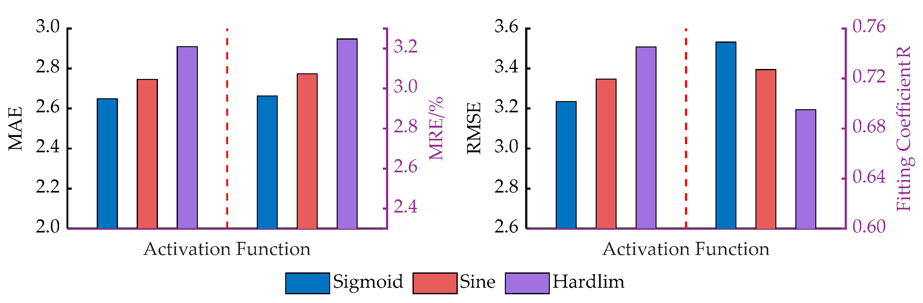
6.4.1. Selection of Activation Functions
Activation functions play a pivotal role in neural networks. Here are some of the most prevalent activation functions in neural networks, including the sigmoid function, the sine function, and the hardlim function [32,33], with specific details provided below:
In light of the findings in Figure 9, utilizing the sigmoid function as the activation function in the extreme learning machine model demonstrates improved learning efficiency and enhanced fitting precision. Following that, the performance of the sine function is observed, while among these three activation functions, the hardlim function displays inferior performance. Therefore, we have opted for the sigmoid function as the activation function for subsequent modeling.
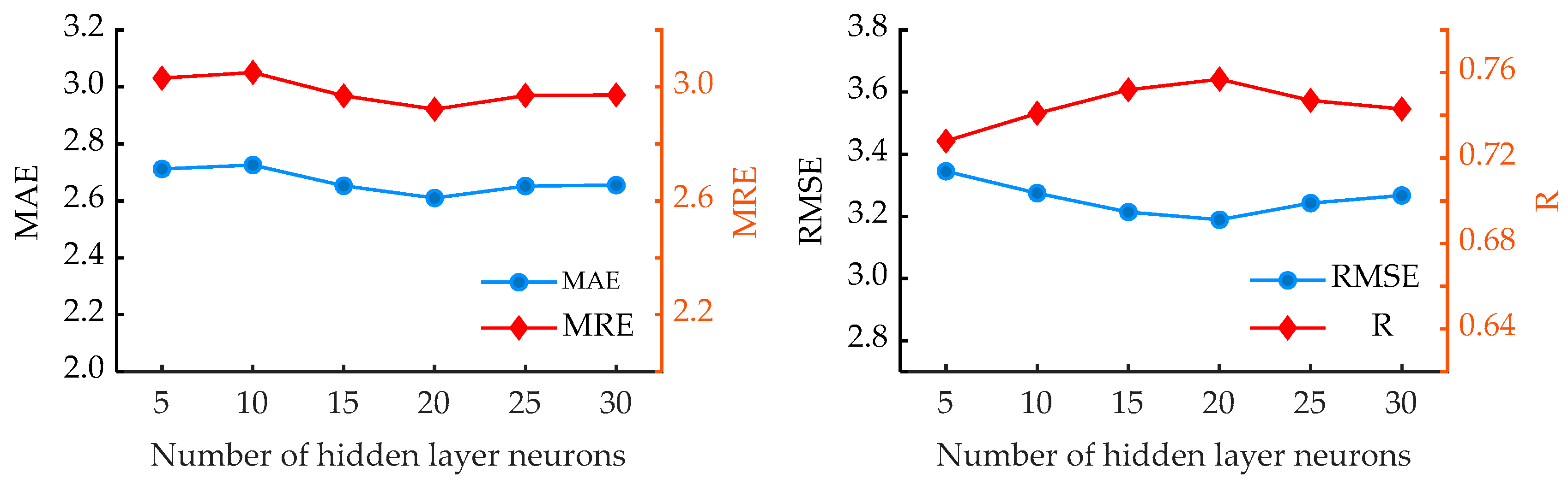
6.4.2. Determining the Number of Neurons in the Neural Network
In this study, we evaluated the predictive accuracy of the ELM model using the sigmoid activation function. The assessment was conducted for various numbers of neurons in the hidden layer, namely, 5, 10, 15, 20, 25, and 30. The obtained accuracy results exhibited a parabolic distribution, and it was observed that the highest accuracy was achieved when the number of neurons was set to 20 in the hidden layer. Consequently, we determined the number of neurons in the hidden layer as 20 for our model. The results are illustrated in Figure 10.
6.5. Forecasting Results and Comparisons
6.5.1. Prediction of BCI of Overall Bridge Structure
Before each training and testing process, a set of 430 data points was randomly chosen as training samples. Additionally, 109 data points were reserved as testing samples. Based on the previous research, the activation function of the ELM algorithm is set to the sigmoid function, with 20 hidden-layer neurons; the WOA population size is set to 20 individuals, and the maximum number of iterations is 50 times.
To mitigate the influence of random sample allocation on predictive results, the best outcome from 10 runs was adopted as the final result. Furthermore, a comparative analysis was conducted to validate the superiority of the proposed method. The analysis involved WOA-ELM, ELM, BPNN, decision trees (DT) and support vector machine (SVM) as the subjects of comparison.
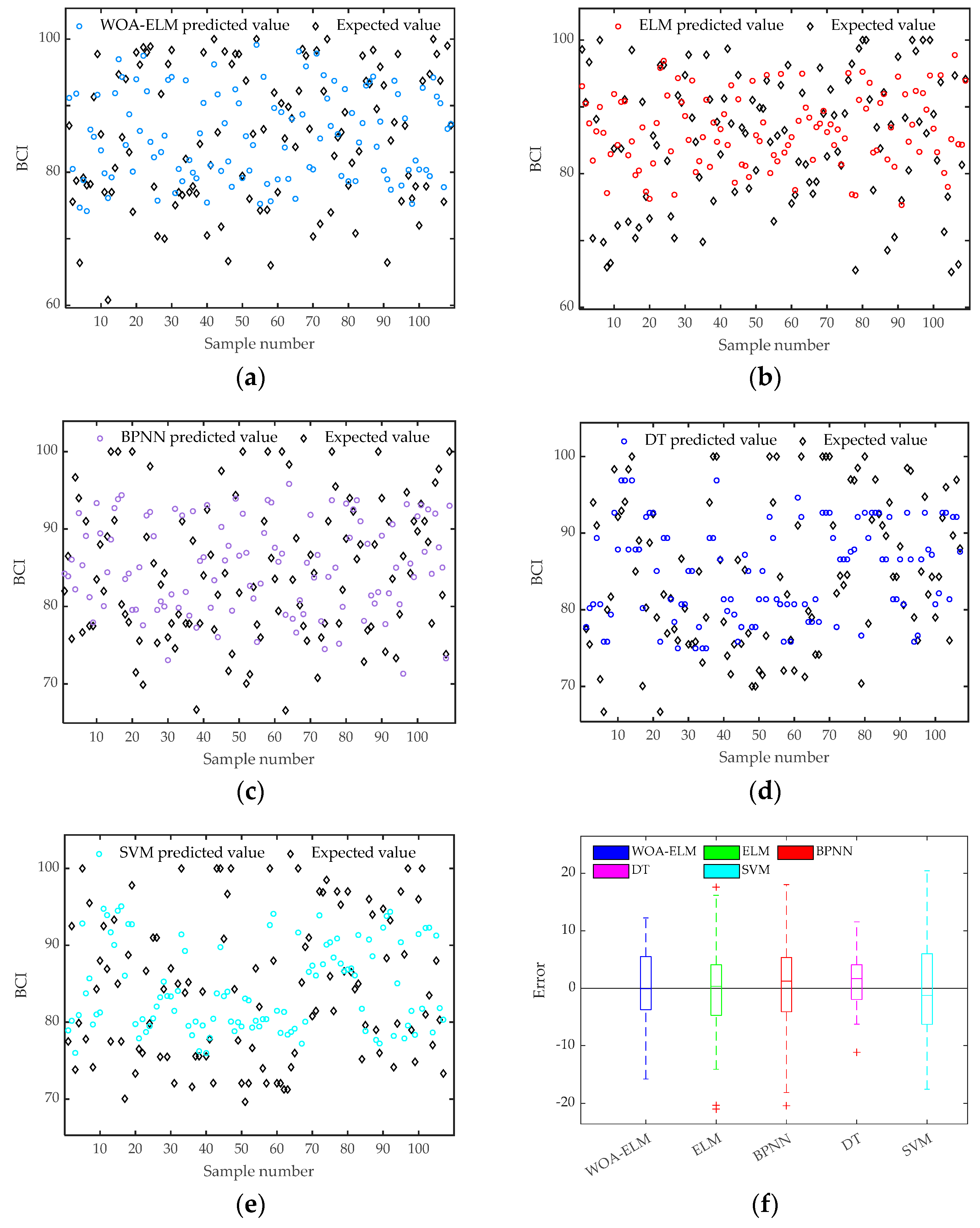
The predictive model’s performance was evaluated using several metrics, including MAE, MRE, RMSE, and R. The comparison between the predicted and expected BCI is illustrated in Figure 11. The input layer of the model comprised 11 neurons, while the output layer consisted of 1 neuron.
Figure 11 reveals differences between the predictions of BCI values for the technical condition of bridges by five different algorithms and their expected values, resulting in a substantial overlap among certain data points. In practice, the predictive models based on the WOA-ELM algorithm and the ELM algorithm demonstrate remarkable proficiency in capturing sample characteristics, and exhibit especially favorable proficiency for forecasting trends in the technical state of bridges. Accurately predicting changes in bridge conditions will aid managers in taking preemptive measures to maintain bridge performance and enhance safety. Additionally, upon closer examination of the prediction error distribution for BCI values among the five algorithms, the WOA-ELM algorithm manages the magnitude of prediction errors significantly, with overall error fluctuations primarily concentrated around values near zero. Following this, the ELM algorithm exhibits relatively lower error levels. However, the SVM and BP neural networks, among the five algorithms, exhibit the most significant overall deviations in prediction errors and possess a larger number of outliers.
Figure 12 portrays scatter plots that exhibit the forecasted and anticipated BCI values, employing five algorithms: WOA-ELM, ELM, BPNN, DT, and SVM. The data points from all five models extend outward around the diagonal line. Additionally, five is a dense distribution near the diagonal, indicating a high degree of agreement between the predicted and expected values. Furthermore, the probability density distribution curves of the BCI prediction errors for the five algorithms are compared. The WOA-ELM algorithm exhibits a smaller extension range and a higher concentration of data points around the peak of the density curve. These observations indicate its superior ability to track the expected values. Moreover, the ELM and DT algorithms show a slightly lower capturing effect on the expected values, and the BPNN and SVM algorithms display a larger dispersion in the distribution of prediction data, indicating poorer control over error fluctuations.
The results depicted in Table 2 reveal significant advancements attained by the WOA-ELM model when compared to the ELM, BPNN, DT, and SVM models. In particular, the WOA-ELM model exhibits significant improvements in R, with enhancements of 4.1%, 11.4%, 24.5%, and 33.6%. Additionally, the model demonstrates reductions in MAE by 9.9%, 13.6%, 5.4%, and 15.7%, and MRE by 11.6%, 15.3%, 6%, and16.2%, respectively. Furthermore, the RMSE is lower by 7.3%, 18.0%, 14.8%, and 18.1% for the corresponding evaluations. The obtained results establish a remarkable level of consistency between the proposed WOA-ELM model and the other four models concerning the predictions of BCI values. When compared to other models, the proposed model exhibits superior performance in various aspects. It shows superiority in terms of both absolute and relative deviations in predictions. Additionally, the proposed model demonstrates better performance in deviation fluctuation and goodness of fit measures. The proposed model exhibits the lowest level of deviation between predicted and expected values. This signifies its high prediction accuracy and remarkable generalization capability. As a result, the model enables the effective forecasting of bridge states under various time points and feature variables. These achievements can be primarily attributed to the optimization of the initial weights and thresholds of the extreme learning machine through the whale optimization algorithm. Following this, the network undergoes training and testing on the dataset with the optimized initial weights and thresholds. As a consequence, commendable performance is achieved in both accuracy and generalization capability.
6.5.2. Prediction of BCI of Bridge Components
Similarly, employing the WOA-ELM model with consistent parameters, predictions were made for the degradation scores of the bridge deck, superstructure, and substructure. A comparative analysis between the predicted BCI and the expected values is presented in Figure 12, Figure 13 and Figure 14. Specifically, the bridge deck model incorporates an input layer consisting of nine neurons, the superstructure model features an input layer comprising eight neurons, and the substructure model is equipped with an input layer comprising seven neurons. Each of these models has an output layer consisting of one neuron.
According to Figure 13, Figure 14 and Figure 15, the WOA-ELM algorithm demonstrates excellent generalization performance and fitting accuracy in the evaluation of various components and overall ratings of bridges. It also exhibits a minimal presence of outliers and high applicability across diverse data features. While the DT model shows low error variance and dispersion in predicting BCI values for upper structural elements, there is room for improvement in other performance aspects. It is worth noting that the model exhibits relatively lower fitting accuracy in the evaluation of lower structural components. This is primarily due to the fact that, within the entire regional road network, most bridge substructures remain in good condition, with no localized minor damage or deterioration. As a result, BCI values tend to be uniformly high, and the variability is low, making the algorithm susceptible to noise interference and, thus, challenging in accurately capturing the relationship between structural states and feature variables. Especially taking bridge decks as an example, the WOA-ELM model demonstrates a significant advantage in terms of R-squared, with improvements of 9.5%, 12.7%, 16.7%, and 19.7%, respectively. Furthermore, the model exhibits reductions of 4.3%, 6.5%, 1.7%, and 12.5% in terms of MAE, and reductions of 6.4%, 6.7%, 2.8%, and 13.3% in terms of MRE. Additionally, the corresponding RMSE evaluations show reductions of 5.4%, 9.0%, 4.3%, and 12.7%, respectively.
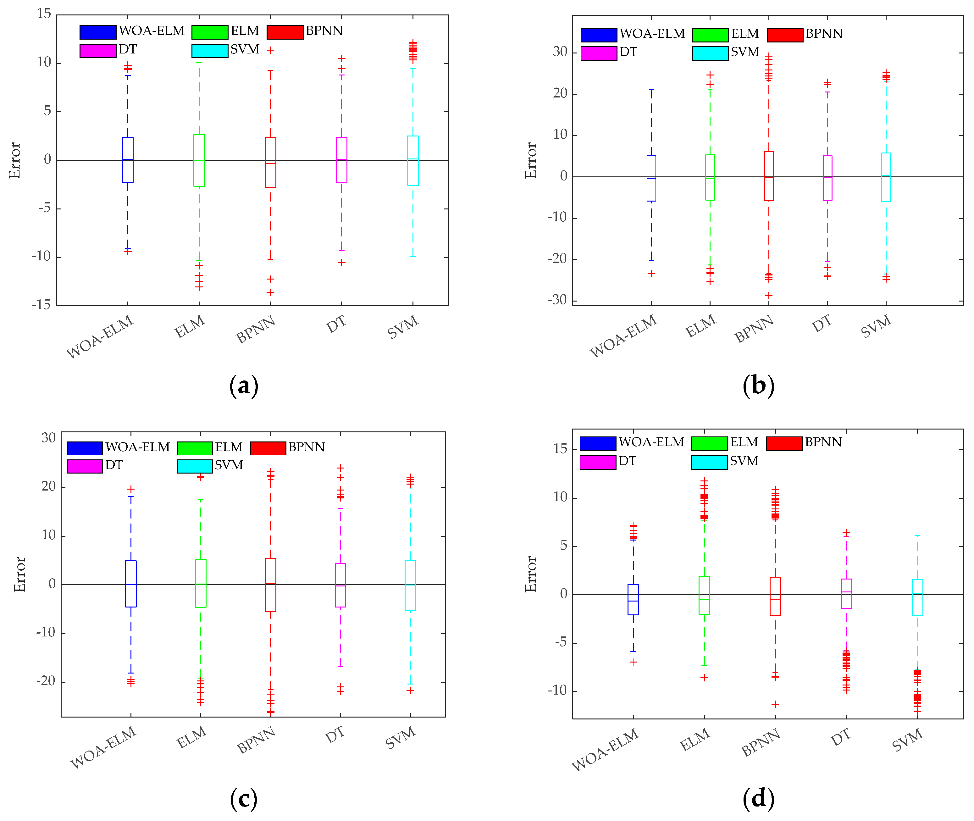
Given that the randomness of the data can affect the model to some extent, we conducted ten random splits of the dataset and generated a box plot of the errors between predicted values and expected values, as illustrated below.
According to Figure 16, after ten runs, the WOA-ELM algorithm demonstrated that the median errors in both the overall bridge structure and component ratings were primarily within proximity to zero, reaffirming the model’s outstanding predictive performance. Additionally, WOA-ELM exhibited the lowest number of outliers among the five models, indicating strong generalization capabilities. While the BPNN and SVM models had relatively good error distributions, the presence of too many outliers was deemed unacceptable. Furthermore, despite the ELM and DT models showcasing solid generalization and accuracy under ideal conditions, an overall examination of ten runs revealed more scattered error distributions and a higher occurrence of outliers, indicative of the lower stability of these two models.
7. Conclusions
In this study, a comprehensive dataset of bridge condition deterioration was meticulously collected by the aggregation of extensive bridge inspection data. The dataset encompasses 11 significant input features, including bridge service time, region, and bridge type. Leveraging this comprehensive dataset, a data-driven WOA-ELM bridge condition deterioration prediction model was successfully constructed. To ensure the reliability and robustness of the proposed method, it was subjected to rigorous validation using a substantial volume of inspection data. The extensive validation process has enabled us to draw the following concluding insights:
- (1)
- The foundation of this study rests upon a comprehensive dataset of bridge inspection data, which facilitates the establishment of complex nonlinear connections between essential features and bridge conditions. This research effectively harnesses and explores the inherent data patterns within the long-term bridge inspection data. Setting itself apart from other prediction models that focus solely on individual bridges, the proposed model demonstrates exceptional proficiency in precisely forecasting the states of diverse bridges within the region.
- (2)
- In this study, we conducted correlation analysis, taking into consideration several key factors, including the bridge’s age, lane count, bridge width, bridge type, structural form, span, bridge length, geographic location, and maintenance status. The aim was to enhance the accuracy of BCI prediction. Furthermore, the WOA-ELM prediction model proposed in this paper outperforms the ELM, BPNN, DT, and SVM models in terms of sample fitting capability and accuracy. Specifically, the model presented in this paper exhibited improvements in R-values by 4.1%, 11.4%, 24.5%, and 33.6%, reductions in RMSE by 7.3%, 18.0%, 14.8%, and 18.1%, decreases in MAE by 9.9%, 13.6%, 5.4%, and 15.7%, and reductions in MRE by 11.6%, 15.3%, 6%, and 16.2%. These results clearly demonstrate a significant enhancement in the model’s performance for bridge condition prediction.
- (3)
- In the context of predicting the BCI for bridge components, we utilized Pearson correlation analysis and mutual information theory to identify the critical influencing factors that need to be taken into account for each specific component. For instance, within the realm of the bridge superstructure, it was imperative to consider variables such as bridge age, lane count, bridge width, bridge type, structural form, span, bridge length, geographic location, and maintenance status. When undertaking the prediction BCI for various bridge components, our proposed method consistently demonstrated remarkable advantages, surpassing the performance of the ELM, BPNN, DT, and SVM models in terms of predictive accuracy. Specifically, with regard to bridge decking components, our method resulted in significant improvements in R-values, with increases of 9.5%, 12.7%, 16.7%, and 19.7%. Additionally, there were reductions in RMSE by 5.4%, 9.0%, 4.3%, and 12.7%, decreases in MAE by 4.3%, 6.5%, 1.7%, and 12.5%, and reductions in MRE by 6.4%, 6.7%, 2.8%, and 13.3%. These outcomes prominently underscore the exceptional predictive prowess of our methodology across diverse bridge component conditions. The significance of this research lies in the provision of a more dependable technical assessment tool for bridge management and maintenance, poised to assume a pivotal role in practical applications.
Although our proposed method exhibits significant advantages over other models, there is still room for further improvement in the predictive performance of our model (e.g., enhancing the optimization precision and learning efficiency of meta-learning). Therefore, we will focus on exploring meta-learning algorithms to further enhance the performance of our model in the field of BCI prediction in future research.
Author Contributions
L.J. contributed to methodology, conceptualization, data curation, formal analysis, investigation, and writing. Q.T. was involved in data curation, methodology, validation and the preparation of the original draft. Y.J. contributed to conceptualization, investigation and supervision. H.C. was involved in conceptualization, the preparation of the original draft, and data collection. Z.X. participated in validation, reviewing and data collection. All authors have read and agreed to the published version of the manuscript.
Funding
This work was supported by the National Natural Science Foundation of China (Grant No. 52278292), the Chongqing Outstanding Youth Science Foundation (Grant No. CSTB2023NSCQ-JQX0029), the Chongqing Science and Technology Project (CSTB2022TIAD-KPX0205), the Chongqing Transportation Science and Technology Project (Grant No. 2022-01), the Science and Technology Project of Guizhou Department of Transportation (Grant No. 2023-122-001), the China Postdoctoral Science Foundation (Grant No. 2023M730431), the Special Funding of Chongqing Postdoctoral Research Project (Grant No. 2022CQBSHTB2053), and the Research and Innovation Program for Graduate Students in Chongqing (Grant No. CYS23477).
Data Availability Statement
The data presented in this study are available on request from the corresponding author.
Conflicts of Interest
The authors declare no conflict of interest.
Appendix A

Table A1.
Dataset.
| NO. | A | B | C | D | E | F | G | H | I | J | K | NO. | A | B | C | D | E | F | G | H | I | J | K |
|---|---|---|---|---|---|---|---|---|---|---|---|---|---|---|---|---|---|---|---|---|---|---|---|
| 1 | 2 | 1 | 4 | 3 | 35 | 365 | 8 | 2 | 0 | 0 | 0 | 271 | 1 | 2 | 13 | 1 | 8 | 20 | 31 | 8 | 0 | 0 | 0 |
| 2 | 1 | 2 | 15 | 1 | 10 | 20 | 25 | 6 | 0 | 1 | 0 | 272 | 1 | 2 | 19 | 1 | 6 | 8.3 | 31 | 8 | 1 | 0 | 0 |
| 3 | 1 | 2 | 10 | 1 | 10 | 20 | 25 | 6 | 1 | 0 | 1 | 273 | 1 | 2 | 13 | 1 | 6 | 8.3 | 31 | 8 | 0 | 0 | 0 |
| 4 | 1 | 2 | 8 | 1 | 10 | 20 | 25 | 6 | 0 | 0 | 0 | 274 | 2 | 2 | 19 | 3 | 21 | 59 | 9 | 1 | 1 | 0 | 0 |
| 5 | 1 | 2 | 12 | 1 | 10 | 21 | 24.5 | 6 | 1 | 1 | 0 | 275 | 2 | 2 | 15 | 3 | 21 | 59 | 9 | 1 | 0 | 0 | 0 |
| 6 | 1 | 2 | 7 | 1 | 10 | 21 | 24.5 | 6 | 0 | 0 | 0 | 276 | 1 | 3 | 16 | 1 | 20 | 39.5 | 33 | 8 | 0 | 1 | 1 |
| 7 | 1 | 2 | 5 | 1 | 10 | 21 | 24.5 | 6 | 0 | 0 | 0 | 277 | 1 | 3 | 13 | 1 | 20 | 39.5 | 33 | 8 | 1 | 0 | 0 |
| 8 | 1 | 2 | 16 | 1 | 20 | 85 | 31 | 8 | 0 | 1 | 0 | 278 | 1 | 3 | 10 | 1 | 20 | 39.5 | 33 | 8 | 0 | 0 | 0 |
| 9 | 1 | 2 | 14 | 1 | 20 | 85 | 31 | 8 | 0 | 0 | 0 | 279 | 1 | 3 | 16 | 1 | 20 | 33 | 31.5 | 8 | 1 | 0 | 0 |
| 10 | 1 | 2 | 18 | 1 | 20 | 52 | 35 | 8 | 0 | 1 | 0 | 280 | 1 | 3 | 13 | 1 | 20 | 33 | 31.5 | 8 | 0 | 1 | 0 |
| 11 | 1 | 2 | 13 | 1 | 20 | 52 | 35 | 8 | 0 | 0 | 0 | 281 | 1 | 3 | 10 | 1 | 20 | 33 | 31.5 | 8 | 0 | 0 | 0 |
| 12 | 1 | 2 | 11 | 1 | 20 | 52 | 35 | 8 | 0 | 0 | 0 | 282 | 1 | 3 | 16 | 2 | 20 | 41 | 31.5 | 8 | 1 | 0 | 0 |
| 13 | 2 | 1 | 4 | 3 | 45 | 45 | 8 | 1 | 0 | 0 | 0 | 283 | 1 | 3 | 13 | 2 | 20 | 41 | 31.5 | 8 | 1 | 0 | 0 |
| 14 | 1 | 3 | 18 | 2 | 40 | 180 | 31.5 | 8 | 1 | 1 | 0 | 284 | 1 | 3 | 16 | 1 | 20 | 35 | 31.5 | 8 | 0 | 1 | 0 |
| 15 | 1 | 3 | 18 | 2 | 30 | 230 | 8.5 | 2 | 1 | 0 | 0 | 285 | 1 | 3 | 13 | 1 | 20 | 35 | 31.5 | 8 | 1 | 0 | 0 |
| 16 | 1 | 3 | 13 | 2 | 30 | 230 | 8.5 | 2 | 0 | 0 | 0 | 286 | 1 | 3 | 10 | 1 | 20 | 35 | 31.5 | 8 | 0 | 0 | 0 |
| 17 | 1 | 3 | 18 | 1 | 20 | 66 | 11 | 3 | 0 | 0 | 0 | 287 | 2 | 2 | 18 | 3 | 19 | 93 | 7 | 1 | 1 | 1 | 0 |
| 18 | 1 | 3 | 13 | 1 | 20 | 66 | 11 | 3 | 0 | 0 | 0 | 288 | 2 | 2 | 14 | 3 | 19 | 93 | 7 | 1 | 0 | 0 | 0 |
| 19 | 1 | 3 | 11 | 1 | 20 | 66 | 11 | 3 | 0 | 0 | 0 | 289 | 1 | 2 | 18 | 3 | 24 | 29 | 7 | 1 | 1 | 0 | 0 |
| 20 | 2 | 3 | 18 | 3 | 20 | 65 | 11 | 3 | 0 | 0 | 0 | 290 | 1 | 2 | 14 | 3 | 24 | 29 | 7 | 1 | 0 | 0 | 0 |
| 21 | 2 | 3 | 13 | 3 | 20 | 65 | 11 | 3 | 0 | 0 | 0 | 291 | 2 | 2 | 18 | 3 | 24 | 176 | 7 | 1 | 1 | 0 | 0 |
| 22 | 2 | 3 | 11 | 3 | 20 | 65 | 11 | 3 | 0 | 0 | 0 | 292 | 2 | 2 | 14 | 3 | 24 | 176 | 7 | 1 | 0 | 0 | 0 |
| 23 | 1 | 3 | 18 | 1 | 20 | 57 | 24.5 | 6 | 1 | 1 | 0 | 293 | 1 | 2 | 13 | 2 | 50 | 768 | 24.5 | 6 | 1 | 0 | 0 |
| 24 | 1 | 3 | 13 | 1 | 20 | 57 | 24.5 | 6 | 1 | 0 | 0 | 294 | 1 | 2 | 10 | 2 | 50 | 768 | 24.5 | 6 | 0 | 0 | 0 |
| 25 | 2 | 1 | 3 | 3 | 23 | 73 | 8 | 1 | 0 | 0 | 0 | 295 | 1 | 3 | 12 | 2 | 40 | 379 | 32.6 | 8 | 1 | 0 | 1 |
| 26 | 1 | 3 | 18 | 1 | 25 | 84 | 19.3 | 4 | 0 | 1 | 0 | 296 | 1 | 3 | 9 | 2 | 40 | 379 | 32.6 | 8 | 0 | 0 | 0 |
| 27 | 2 | 1 | 3 | 3 | 40 | 289 | 35 | 8 | 0 | 0 | 0 | 297 | 1 | 3 | 7 | 2 | 40 | 379 | 32.6 | 8 | 0 | 0 | 0 |
| 28 | 2 | 3 | 18 | 3 | 24 | 236 | 9.5 | 2 | 1 | 1 | 0 | 298 | 2 | 2 | 11 | 3 | 30 | 350 | 10 | 2 | 0 | 0 | 1 |
| 29 | 2 | 3 | 13 | 3 | 24 | 236 | 9.5 | 2 | 0 | 0 | 0 | 299 | 2 | 2 | 8 | 3 | 30 | 350 | 10 | 2 | 0 | 0 | 0 |
| 30 | 2 | 3 | 11 | 3 | 24 | 236 | 9.5 | 2 | 0 | 0 | 0 | 300 | 1 | 2 | 19 | 2 | 30 | 234 | 31 | 8 | 0 | 0 | 0 |
| 31 | 1 | 3 | 18 | 1 | 20 | 29 | 24.5 | 6 | 1 | 0 | 0 | 301 | 1 | 2 | 14 | 2 | 30 | 234 | 31 | 8 | 0 | 0 | 0 |
| 32 | 1 | 3 | 13 | 1 | 20 | 29 | 24.5 | 6 | 1 | 0 | 0 | 302 | 1 | 3 | 16 | 2 | 20 | 59 | 31.5 | 8 | 1 | 1 | 0 |
| 33 | 2 | 1 | 20 | 3 | 40 | 100 | 16 | 3 | 0 | 0 | 0 | 303 | 1 | 3 | 16 | 2 | 20 | 125 | 31.5 | 8 | 1 | 1 | 0 |
| 34 | 2 | 1 | 15 | 3 | 40 | 100 | 16 | 3 | 1 | 0 | 0 | 304 | 2 | 2 | 20 | 3 | 20 | 111 | 8 | 2 | 0 | 1 | 0 |
| 35 | 2 | 1 | 14 | 3 | 40 | 100 | 16 | 3 | 1 | 0 | 0 | 305 | 1 | 2 | 20 | 1 | 16 | 192 | 7 | 1 | 0 | 0 | 0 |
| 36 | 2 | 1 | 12 | 3 | 40 | 100 | 16 | 3 | 0 | 0 | 0 | 306 | 1 | 3 | 16 | 2 | 20 | 95 | 31.5 | 8 | 1 | 1 | |
| 37 | 1 | 1 | 20 | 1 | 20 | 35 | 31 | 6 | 1 | 0 | 0 | 307 | 1 | 3 | 13 | 2 | 20 | 95 | 31.5 | 8 | 0 | 0 | 0 |
| 38 | 1 | 1 | 15 | 1 | 20 | 35 | 31 | 6 | 0 | 0 | 0 | 308 | 1 | 3 | 11 | 2 | 20 | 95 | 31.5 | 8 | 0 | 0 | 0 |
| 39 | 1 | 1 | 14 | 1 | 20 | 35 | 31 | 6 | 0 | 0 | 0 | 309 | 2 | 1 | 4 | 3 | 25 | 194 | 9 | 2 | 1 | 0 | 0 |
| 40 | 1 | 1 | 12 | 1 | 20 | 35 | 31 | 6 | 0 | 0 | 0 | 310 | 2 | 1 | 4 | 3 | 24 | 57 | 9 | 2 | 0 | 0 | 0 |
| 41 | 2 | 1 | 3 | 3 | 23 | 73 | 8 | 1 | 0 | 0 | 0 | 311 | 1 | 3 | 16 | 2 | 20 | 94 | 31.5 | 8 | 0 | 1 | 1 |
| 42 | 1 | 1 | 20 | 3 | 20 | 54 | 31 | 6 | 0 | 1 | 0 | 312 | 1 | 3 | 13 | 2 | 20 | 94 | 31.5 | 8 | 1 | 0 | 0 |
| 43 | 1 | 1 | 15 | 3 | 20 | 54 | 31 | 6 | 1 | 0 | 0 | 313 | 2 | 2 | 4 | 3 | 28 | 62 | 9 | 2 | 0 | 0 | 0 |
| 44 | 1 | 1 | 12 | 3 | 20 | 54 | 31 | 6 | 0 | 0 | 0 | 314 | 2 | 2 | 4 | 3 | 34 | 263 | 9 | 2 | 1 | 0 | 0 |
| 45 | 1 | 1 | 20 | 2 | 25 | 38 | 31 | 6 | 0 | 0 | 0 | 315 | 2 | 2 | 4 | 3 | 29 | 236 | 9 | 2 | 0 | 0 | 0 |
| 46 | 1 | 1 | 15 | 2 | 25 | 38 | 31 | 6 | 1 | 0 | 0 | 316 | 2 | 2 | 4 | 3 | 35 | 122 | 9 | 2 | 0 | 0 | 0 |
| 47 | 1 | 1 | 14 | 2 | 25 | 38 | 31 | 6 | 1 | 1 | 0 | 317 | 2 | 2 | 4 | 3 | 36 | 52 | 9 | 2 | 0 | 0 | 0 |
| 48 | 1 | 1 | 12 | 2 | 25 | 38 | 31 | 6 | 0 | 0 | 0 | 318 | 2 | 2 | 4 | 3 | 35 | 265 | 9 | 2 | 0 | 0 | 0 |
| 49 | 2 | 1 | 4 | 3 | 35 | 275 | 8 | 1 | 0 | 0 | 0 | 319 | 2 | 2 | 18 | 2 | 20 | 94 | 31.5 | 8 | 0 | 0 | 0 |
| 50 | 2 | 1 | 3 | 3 | 30 | 42 | 9 | 2 | 0 | 0 | 0 | 320 | 2 | 2 | 15 | 2 | 20 | 94 | 31.5 | 8 | 1 | 0 | 0 |
| 51 | 2 | 1 | 3 | 3 | 35 | 111 | 9 | 2 | 0 | 0 | 0 | 321 | 2 | 2 | 18 | 3 | 28 | 294 | 7 | 1 | 0 | 0 | 0 |
| 52 | 2 | 3 | 6 | 3 | 27 | 207 | 8 | 2 | 0 | 0 | 0 | 322 | 2 | 2 | 15 | 3 | 28 | 294 | 7 | 1 | 1 | 0 | 0 |
| 53 | 2 | 1 | 3 | 3 | 33 | 72 | 9 | 2 | 0 | 0 | 0 | 323 | 2 | 2 | 18 | 3 | 38 | 288 | 9 | 2 | 0 | 0 | 0 |
| 54 | 2 | 1 | 3 | 3 | 24 | 420 | 9 | 2 | 0 | 0 | 0 | 324 | 2 | 2 | 15 | 3 | 38 | 288 | 9 | 2 | 1 | 0 | 0 |
| 55 | 2 | 2 | 3 | 3 | 20 | 90 | 9 | 2 | 0 | 0 | 0 | 325 | 2 | 2 | 14 | 3 | 35 | 133 | 7 | 1 | 1 | 0 | 0 |
| 56 | 2 | 1 | 3 | 3 | 37.5 | 373 | 11.5 | 2 | 0 | 0 | 0 | 326 | 2 | 2 | 14 | 3 | 33 | 153 | 5.5 | 1 | 0 | 0 | 0 |
| 57 | 2 | 1 | 3 | 3 | 24 | 68 | 7 | 1 | 0 | 0 | 0 | 327 | 2 | 2 | 18 | 3 | 24 | 176 | 7 | 1 | 0 | 1 | 0 |
| 58 | 2 | 1 | 3 | 3 | 27 | 407 | 9 | 2 | 0 | 0 | 0 | 328 | 2 | 2 | 15 | 3 | 24 | 176 | 7 | 1 | 1 | 0 | 0 |
| 59 | 2 | 1 | 4 | 3 | 35 | 465 | 9 | 2 | 0 | 0 | 0 | 329 | 2 | 2 | 18 | 3 | 33 | 262 | 9 | 2 | 0 | 1 | 0 |
| 60 | 2 | 3 | 6 | 3 | 37 | 150 | 8 | 2 | 0 | 0 | 0 | 330 | 2 | 2 | 15 | 3 | 33 | 262 | 9 | 2 | 0 | 0 | 0 |
| 61 | 2 | 3 | 4 | 3 | 37 | 491 | 6 | 1 | 0 | 0 | 0 | 331 | 2 | 2 | 18 | 3 | 23 | 204 | 9.5 | 2 | 1 | 0 | 0 |
| 62 | 2 | 3 | 6 | 3 | 46 | 171 | 11.7 | 2 | 0 | 0 | 0 | 332 | 2 | 2 | 15 | 3 | 23 | 204 | 9.5 | 2 | 0 | 0 | 0 |
| 63 | 2 | 1 | 5 | 3 | 32 | 443 | 13 | 3 | 0 | 0 | 0 | 333 | 2 | 2 | 14 | 3 | 23 | 204 | 9.5 | 2 | 1 | 0 | 0 |
| 64 | 2 | 3 | 6 | 3 | 30 | 142 | 8 | 2 | 0 | 0 | 0 | 334 | 2 | 2 | 18 | 3 | 23 | 140 | 14.5 | 3 | 0 | 0 | 0 |
| 65 | 2 | 3 | 2 | 3 | 33 | 391 | 7 | 1 | 0 | 0 | 0 | 335 | 2 | 2 | 18 | 3 | 28 | 294 | 9.5 | 2 | 0 | 0 | 0 |
| 66 | 2 | 3 | 6 | 3 | 27 | 118 | 9 | 1 | 0 | 0 | 0 | 336 | 1 | 2 | 18 | 3 | 24 | 29 | 13 | 2 | 0 | 0 | 0 |
| 67 | 2 | 3 | 6 | 3 | 29 | 289 | 9 | 2 | 0 | 0 | 0 | 337 | 2 | 2 | 18 | 3 | 38 | 288 | 9 | 2 | 0 | 1 | 0 |
| 68 | 2 | 3 | 6 | 3 | 38 | 238 | 12.8 | 2 | 0 | 0 | 0 | 338 | 2 | 2 | 18 | 3 | 28 | 294 | 7 | 1 | 1 | 0 | 0 |
| 69 | 2 | 3 | 4 | 3 | 40 | 526 | 7 | 1 | 0 | 0 | 0 | 339 | 2 | 2 | 18 | 3 | 24 | 176 | 7 | 1 | 1 | 0 | 0 |
| 70 | 2 | 3 | 4 | 3 | 50 | 660 | 7 | 1 | 0 | 0 | 0 | 340 | 2 | 2 | 5 | 3 | 25 | 157 | 8 | 1 | 0 | 0 | 0 |
| 71 | 2 | 3 | 2 | 3 | 39 | 228 | 7 | 1 | 0 | 0 | 0 | 341 | 2 | 2 | 5 | 3 | 26 | 270 | 8 | 1 | 0 | 0 | 0 |
| 72 | 2 | 3 | 4 | 3 | 39 | 400 | 7 | 1 | 0 | 0 | 0 | 342 | 2 | 2 | 5 | 3 | 28 | 171 | 8 | 1 | 0 | 0 | 0 |
| 73 | 2 | 3 | 2 | 3 | 36 | 530 | 7 | 1 | 0 | 0 | 0 | 343 | 2 | 2 | 5 | 3 | 25 | 25 | 13.5 | 3 | 0 | 0 | 0 |
| 74 | 2 | 3 | 4 | 3 | 39 | 618 | 7 | 1 | 0 | 0 | 0 | 344 | 2 | 2 | 5 | 3 | 30 | 243 | 8 | 1 | 0 | 0 | 0 |
| 75 | 2 | 3 | 2 | 3 | 32 | 370 | 7 | 1 | 0 | 0 | 0 | 345 | 2 | 2 | 5 | 3 | 31 | 301 | 8 | 1 | 0 | 0 | 0 |
| 76 | 2 | 3 | 2 | 3 | 38 | 645 | 9 | 2 | 0 | 0 | 0 | 346 | 2 | 2 | 5 | 3 | 28 | 233 | 8 | 1 | 0 | 0 | 0 |
| 77 | 2 | 3 | 2 | 3 | 50 | 580 | 9 | 2 | 0 | 0 | 0 | 347 | 2 | 2 | 11 | 3 | 20 | 292 | 9.5 | 2 | 0 | 0 | 0 |
| 78 | 2 | 3 | 2 | 3 | 30 | 238 | 7 | 1 | 0 | 0 | 0 | 348 | 2 | 2 | 12 | 3 | 20 | 109 | 9 | 2 | 0 | 0 | 0 |
| 79 | 2 | 3 | 4 | 3 | 36 | 147 | 7 | 1 | 0 | 0 | 0 | 349 | 1 | 2 | 11 | 2 | 40 | 430 | 24.5 | 6 | 0 | 0 | 0 |
| 80 | 2 | 3 | 4 | 3 | 50 | 465 | 9.5 | 2 | 0 | 0 | 0 | 350 | 1 | 2 | 7 | 2 | 40 | 430 | 24.5 | 6 | 0 | 0 | 0 |
| 81 | 2 | 1 | 4 | 3 | 36 | 350 | 10 | 2 | 0 | 0 | 0 | 351 | 1 | 1 | 20 | 1 | 20 | 58 | 31 | 6 | 1 | 0 | 0 |
| 82 | 2 | 1 | 3 | 3 | 32 | 452 | 27 | 6 | 0 | 0 | 0 | 352 | 1 | 1 | 17 | 1 | 20 | 58 | 31 | 6 | 0 | 0 | 0 |
| 83 | 2 | 1 | 5 | 3 | 32 | 1038 | 9 | 2 | 0 | 0 | 0 | 353 | 1 | 2 | 19 | 1 | 20 | 31 | 31 | 8 | 0 | 0 | 0 |
| 84 | 1 | 1 | 3 | 3 | 30 | 46 | 40 | 8 | 0 | 0 | 0 | 354 | 1 | 2 | 16 | 1 | 20 | 31 | 31 | 8 | 1 | 0 | 0 |
| 85 | 2 | 3 | 6 | 3 | 54 | 285 | 9.5 | 2 | 0 | 0 | 0 | 355 | 1 | 2 | 14 | 1 | 20 | 31 | 31 | 8 | 0 | 1 | 0 |
| 86 | 2 | 1 | 4 | 3 | 35 | 115 | 17.5 | 4 | 0 | 0 | 0 | 356 | 2 | 3 | 4 | 3 | 30 | 71 | 35 | 6 | 0 | 0 | 0 |
| 87 | 1 | 1 | 4 | 3 | 36 | 151 | 35 | 8 | 0 | 0 | 0 | 357 | 1 | 2 | 17 | 1 | 20 | 70 | 16 | 4 | 0 | 0 | 0 |
| 88 | 2 | 1 | 4 | 3 | 40 | 168 | 35 | 8 | 0 | 0 | 0 | 358 | 2 | 2 | 17 | 3 | 30 | 150 | 9.5 | 2 | 0 | 0 | 0 |
| 89 | 2 | 1 | 4 | 3 | 40 | 168 | 35 | 8 | 0 | 0 | 0 | 359 | 2 | 2 | 9 | 3 | 32 | 220 | 19.5 | 4 | 0 | 0 | 0 |
| 90 | 2 | 1 | 4 | 3 | 35 | 325 | 35 | 8 | 0 | 0 | 0 | 360 | 2 | 2 | 9 | 3 | 40 | 311 | 19.5 | 4 | 0 | 0 | 0 |
| 91 | 2 | 1 | 4 | 3 | 35 | 180 | 17.5 | 4 | 0 | 0 | 0 | 361 | 1 | 2 | 9 | 2 | 35 | 437 | 20 | 4 | 0 | 0 | 0 |
| 92 | 1 | 1 | 4 | 3 | 36 | 396 | 40 | 8 | 0 | 0 | 0 | 362 | 2 | 2 | 9 | 3 | 30 | 120 | 9.5 | 2 | 0 | 0 | 0 |
| 93 | 2 | 1 | 3 | 3 | 35 | 259 | 37 | 8 | 0 | 0 | 0 | 363 | 2 | 2 | 9 | 3 | 33 | 258 | 19.5 | 4 | 0 | 0 | 0 |
| 94 | 2 | 1 | 3 | 3 | 28 | 340 | 10 | 2 | 0 | 0 | 0 | 364 | 2 | 1 | 9 | 3 | 22 | 27 | 9 | 2 | 0 | 0 | 0 |
| 95 | 2 | 1 | 3 | 3 | 35 | 145 | 11.5 | 2 | 0 | 0 | 0 | 365 | 2 | 1 | 9 | 3 | 47 | 148 | 9 | 2 | 0 | 0 | 0 |
| 96 | 2 | 1 | 3 | 3 | 31 | 475 | 11.5 | 2 | 0 | 0 | 0 | 366 | 2 | 1 | 9 | 3 | 32 | 126 | 9 | 2 | 0 | 0 | 0 |
| 97 | 2 | 1 | 3 | 3 | 42 | 130 | 11.5 | 2 | 0 | 0 | 0 | 367 | 2 | 1 | 9 | 3 | 30 | 400 | 9 | 2 | 0 | 0 | 0 |
| 98 | 1 | 1 | 3 | 2 | 40 | 296 | 21 | 4 | 0 | 0 | 0 | 368 | 2 | 1 | 9 | 3 | 33 | 182 | 9 | 2 | 0 | 0 | 0 |
| 99 | 2 | 1 | 3 | 3 | 30 | 367 | 9 | 2 | 0 | 0 | 0 | 369 | 2 | 1 | 9 | 3 | 35 | 345 | 9 | 2 | 1 | 1 | 0 |
| 100 | 2 | 1 | 3 | 3 | 31 | 72 | 9 | 2 | 0 | 0 | 0 | 370 | 2 | 1 | 9 | 3 | 35 | 170 | 9 | 2 | 0 | 0 | 0 |
| 101 | 2 | 1 | 3 | 3 | 35 | 321 | 9 | 2 | 0 | 0 | 0 | 371 | 2 | 1 | 9 | 3 | 30 | 106 | 9 | 2 | 0 | 0 | 0 |
| 102 | 2 | 1 | 3 | 3 | 35 | 328 | 9 | 2 | 0 | 0 | 0 | 372 | 2 | 1 | 9 | 3 | 30 | 1650 | 18.5 | 4 | 0 | 0 | 0 |
| 103 | 1 | 3 | 20 | 2 | 20 | 162 | 15.8 | 4 | 1 | 1 | 0 | 373 | 2 | 1 | 9 | 3 | 30 | 353 | 18.5 | 4 | 1 | 0 | 0 |
| 104 | 2 | 1 | 5 | 3 | 30 | 124 | 8 | 1 | 0 | 0 | 0 | 374 | 2 | 1 | 9 | 3 | 30 | 1560 | 18.5 | 4 | 0 | 0 | 0 |
| 105 | 2 | 1 | 5 | 3 | 35 | 115 | 33 | 8 | 0 | 0 | 0 | 375 | 2 | 1 | 9 | 3 | 33 | 626 | 18.5 | 4 | 1 | 0 | 0 |
| 106 | 2 | 1 | 5 | 3 | 32 | 128 | 8 | 1 | 0 | 0 | 0 | 376 | 2 | 1 | 7 | 3 | 38 | 113 | 11.5 | 2 | 1 | 0 | 0 |
| 107 | 2 | 1 | 4 | 3 | 30 | 120 | 8 | 1 | 0 | 0 | 0 | 377 | 2 | 1 | 4 | 3 | 38 | 113 | 11.5 | 2 | 0 | 0 | 0 |
| 108 | 1 | 1 | 4 | 3 | 36 | 617 | 37 | 8 | 0 | 0 | 0 | 378 | 2 | 1 | 7 | 3 | 40 | 1537 | 21.5 | 4 | 0 | 0 | 0 |
| 109 | 2 | 1 | 4 | 3 | 35 | 285 | 8 | 1 | 0 | 0 | 0 | 379 | 2 | 1 | 4 | 3 | 40 | 1537 | 21.5 | 4 | 0 | 0 | 0 |
| 110 | 2 | 2 | 3 | 3 | 30 | 197 | 9 | 2 | 0 | 0 | 0 | 380 | 2 | 1 | 7 | 3 | 40 | 245 | 11.5 | 2 | 1 | 0 | 0 |
| 111 | 2 | 2 | 3 | 3 | 30 | 373 | 9 | 2 | 0 | 0 | 0 | 381 | 2 | 1 | 4 | 3 | 40 | 245 | 11.5 | 2 | 0 | 0 | 0 |
| 112 | 2 | 2 | 3 | 3 | 31 | 70 | 38 | 8 | 0 | 0 | 0 | 382 | 2 | 1 | 7 | 3 | 30 | 190 | 8 | 1 | 1 | 0 | 0 |
| 113 | 1 | 3 | 18 | 2 | 40 | 260 | 31.5 | 8 | 0 | 1 | 0 | 383 | 2 | 1 | 13 | 3 | 30 | 343 | 10 | 1 | 1 | 0 | 0 |
| 114 | 1 | 3 | 13 | 2 | 40 | 260 | 31.5 | 8 | 1 | 0 | 0 | 384 | 2 | 1 | 7 | 3 | 29 | 143 | 8 | 1 | 1 | 0 | 0 |
| 115 | 1 | 3 | 11 | 2 | 40 | 260 | 31.5 | 8 | 0 | 0 | 0 | 385 | 2 | 1 | 13 | 3 | 23 | 155 | 8 | 1 | 1 | 0 | 0 |
| 116 | 1 | 3 | 14 | 1 | 20 | 28 | 20 | 4 | 1 | 0 | 0 | 386 | 2 | 1 | 13 | 3 | 22 | 276 | 8.5 | 1 | 1 | 0 | 0 |
| 117 | 1 | 3 | 12 | 1 | 20 | 28 | 20 | 4 | 0 | 0 | 0 | 387 | 2 | 1 | 13 | 3 | 30 | 310 | 8 | 1 | 1 | 0 | 0 |
| 118 | 1 | 3 | 18 | 2 | 40 | 400 | 31.5 | 8 | 0 | 0 | 0 | 388 | 2 | 1 | 9 | 3 | 23 | 61 | 8 | 1 | 1 | 0 | 0 |
| 119 | 1 | 3 | 13 | 2 | 40 | 400 | 31.5 | 8 | 0 | 1 | 0 | 389 | 2 | 1 | 6 | 3 | 23 | 61 | 8 | 1 | 0 | 0 | 0 |
| 120 | 1 | 3 | 11 | 2 | 40 | 400 | 31.5 | 8 | 0 | 0 | 0 | 390 | 2 | 1 | 9 | 3 | 25 | 180 | 8 | 1 | 1 | 0 | 0 |
| 121 | 1 | 3 | 18 | 1 | 20 | 20 | 31 | 8 | 0 | 0 | 0 | 391 | 2 | 1 | 6 | 3 | 25 | 180 | 8 | 1 | 0 | 0 | 0 |
| 122 | 1 | 3 | 13 | 1 | 20 | 20 | 31 | 8 | 1 | 1 | 0 | 392 | 2 | 1 | 9 | 3 | 33 | 171 | 8 | 1 | 1 | 0 | 0 |
| 123 | 1 | 3 | 11 | 1 | 20 | 20 | 31 | 8 | 0 | 0 | 0 | 393 | 2 | 1 | 6 | 3 | 33 | 171 | 8 | 1 | 0 | 0 | 0 |
| 124 | 1 | 3 | 18 | 1 | 16 | 27 | 32.5 | 8 | 1 | 0 | 0 | 394 | 2 | 1 | 9 | 3 | 25 | 74 | 8 | 1 | 0 | 0 | 0 |
| 125 | 1 | 3 | 13 | 1 | 16 | 27 | 32.5 | 8 | 1 | 0 | 0 | 395 | 2 | 1 | 6 | 3 | 25 | 74 | 8 | 1 | 0 | 0 | 0 |
| 126 | 1 | 3 | 11 | 1 | 16 | 27 | 32.5 | 8 | 0 | 0 | 0 | 396 | 2 | 1 | 9 | 3 | 25 | 92 | 8 | 1 | 1 | 0 | 0 |
| 127 | 2 | 3 | 18 | 3 | 24 | 403 | 9.5 | 2 | 0 | 0 | 0 | 397 | 2 | 1 | 6 | 3 | 25 | 92 | 8 | 1 | 0 | 0 | 0 |
| 128 | 2 | 3 | 18 | 3 | 24 | 419 | 9.5 | 2 | 0 | 0 | 0 | 398 | 2 | 1 | 9 | 3 | 25 | 191 | 8 | 1 | 1 | 0 | 0 |
| 129 | 1 | 3 | 18 | 1 | 16 | 73 | 31.5 | 8 | 0 | 0 | 0 | 399 | 2 | 1 | 6 | 3 | 25 | 191 | 8 | 1 | 0 | 0 | 0 |
| 130 | 2 | 3 | 18 | 3 | 24 | 138 | 15.8 | 4 | 1 | 0 | 0 | 400 | 2 | 1 | 9 | 3 | 30 | 278 | 8 | 1 | 1 | 0 | 1 |
| 131 | 2 | 3 | 13 | 3 | 24 | 138 | 15.8 | 4 | 0 | 0 | 0 | 401 | 2 | 1 | 6 | 3 | 30 | 278 | 8 | 1 | 0 | 0 | 0 |
| 132 | 2 | 3 | 11 | 3 | 24 | 138 | 15.8 | 4 | 0 | 0 | 0 | 402 | 2 | 1 | 9 | 3 | 25 | 100 | 8 | 1 | 0 | 0 | 0 |
| 133 | 2 | 1 | 10 | 3 | 25 | 100 | 12.5 | 2 | 0 | 0 | 0 | 403 | 2 | 1 | 6 | 3 | 25 | 100 | 8 | 1 | 0 | 0 | 0 |
| 134 | 1 | 3 | 17 | 1 | 20 | 37 | 31 | 8 | 1 | 0 | 1 | 404 | 2 | 2 | 11 | 3 | 33 | 90 | 7.8 | 1 | 0 | 0 | 0 |
| 135 | 1 | 3 | 12 | 1 | 20 | 37 | 31 | 8 | 0 | 0 | 0 | 405 | 2 | 2 | 11 | 3 | 30 | 90 | 7.8 | 1 | 0 | 0 | 0 |
| 136 | 1 | 3 | 10 | 1 | 20 | 37 | 31 | 8 | 0 | 0 | 0 | 406 | 2 | 2 | 11 | 3 | 30 | 30 | 7.8 | 1 | 0 | 0 | 0 |
| 137 | 1 | 3 | 17 | 1 | 30 | 74 | 19 | 4 | 1 | 0 | 0 | 407 | 2 | 2 | 11 | 3 | 30 | 40 | 17.8 | 4 | 0 | 0 | 0 |
| 138 | 1 | 3 | 12 | 1 | 30 | 74 | 19 | 4 | 0 | 0 | 0 | 408 | 2 | 2 | 11 | 3 | 30 | 40 | 17.8 | 4 | 0 | 0 | 0 |
| 139 | 1 | 3 | 10 | 1 | 30 | 74 | 19 | 4 | 0 | 0 | 0 | 409 | 2 | 2 | 11 | 3 | 35 | 110 | 7.8 | 1 | 0 | 0 | 0 |
| 140 | 1 | 3 | 18 | 1 | 25 | 30 | 29 | 8 | 1 | 0 | 0 | 410 | 2 | 2 | 11 | 3 | 33 | 350 | 7.8 | 1 | 0 | 0 | 0 |
| 141 | 1 | 3 | 13 | 1 | 25 | 30 | 29 | 8 | 0 | 1 | 0 | 411 | 2 | 2 | 11 | 3 | 30 | 30 | 7.8 | 1 | 0 | 0 | 0 |
| 142 | 1 | 3 | 11 | 1 | 25 | 30 | 29 | 8 | 0 | 0 | 0 | 412 | 2 | 2 | 7 | 3 | 40 | 374 | 9.5 | 2 | 0 | 0 | 0 |
| 143 | 1 | 2 | 18 | 1 | 20 | 20 | 30 | 8 | 1 | 0 | 0 | 413 | 2 | 2 | 7 | 3 | 38 | 440 | 9.5 | 2 | 1 | 0 | 0 |
| 144 | 1 | 2 | 13 | 1 | 20 | 20 | 30 | 8 | 0 | 1 | 0 | 414 | 2 | 2 | 4 | 3 | 38 | 440 | 9.5 | 2 | 0 | 0 | 0 |
| 145 | 1 | 2 | 11 | 1 | 20 | 20 | 30 | 8 | 0 | 0 | 0 | 415 | 2 | 2 | 7 | 3 | 18 | 70 | 8 | 1 | 0 | 0 | 0 |
| 146 | 1 | 3 | 18 | 1 | 13 | 13 | 31 | 8 | 1 | 0 | 1 | 416 | 2 | 2 | 7 | 3 | 17 | 38 | 8 | 1 | 0 | 0 | 0 |
| 147 | 1 | 3 | 13 | 1 | 13 | 13 | 31 | 8 | 0 | 0 | 0 | 417 | 2 | 1 | 11 | 3 | 35 | 80 | 41.5 | 8 | 0 | 0 | 0 |
| 148 | 1 | 3 | 11 | 1 | 13 | 13 | 31 | 8 | 0 | 0 | 0 | 418 | 2 | 1 | 9 | 3 | 30 | 105 | 33 | 8 | 0 | 0 | 0 |
| 149 | 1 | 1 | 16 | 1 | 20 | 50 | 31 | 8 | 1 | 1 | 0 | 419 | 2 | 1 | 6 | 3 | 20 | 40 | 8 | 2 | 0 | 0 | 0 |
| 150 | 1 | 1 | 14 | 1 | 20 | 50 | 31 | 8 | 0 | 0 | 0 | 420 | 2 | 1 | 9 | 3 | 30 | 252 | 8 | 2 | 0 | 0 | 0 |
| 151 | 1 | 1 | 19 | 1 | 20 | 50 | 16 | 4 | 1 | 0 | 0 | 421 | 2 | 3 | 9 | 3 | 25 | 100 | 31.5 | 8 | 1 | 0 | 0 |
| 152 | 1 | 1 | 14 | 1 | 20 | 50 | 16 | 4 | 0 | 1 | 1 | 422 | 2 | 3 | 9 | 3 | 31 | 98 | 12.5 | 2 | 1 | 1 | 0 |
| 153 | 1 | 1 | 11 | 1 | 20 | 50 | 16 | 4 | 0 | 0 | 0 | 423 | 2 | 1 | 6 | 3 | 45 | 305 | 24.5 | 6 | 0 | 0 | 0 |
| 154 | 1 | 1 | 19 | 1 | 20 | 50 | 16 | 4 | 0 | 0 | 1 | 424 | 2 | 1 | 6 | 3 | 45 | 90 | 14 | 2 | 0 | 1 | 0 |
| 155 | 1 | 1 | 14 | 1 | 20 | 50 | 16 | 4 | 1 | 0 | 0 | 425 | 2 | 1 | 6 | 3 | 46 | 97 | 14 | 2 | 0 | 0 | 0 |
| 156 | 1 | 2 | 15 | 1 | 16 | 60 | 12.3 | 3 | 0 | 0 | 1 | 426 | 1 | 1 | 7 | 3 | 25 | 125 | 9 | 2 | 1 | 0 | 0 |
| 157 | 1 | 2 | 10 | 1 | 16 | 60 | 12.3 | 3 | 0 | 1 | 0 | 427 | 2 | 1 | 13 | 3 | 30 | 90 | 22 | 4 | 0 | 0 | 0 |
| 158 | 1 | 2 | 9 | 1 | 16 | 60 | 12.3 | 3 | 0 | 0 | 0 | 428 | 2 | 1 | 12 | 3 | 33 | 450 | 13 | 2 | 0 | 0 | 0 |
| 159 | 1 | 2 | 15 | 1 | 16 | 24 | 12.3 | 3 | 0 | 0 | 0 | 429 | 2 | 2 | 14 | 3 | 30 | 78 | 13 | 2 | 1 | 0 | 0 |
| 160 | 1 | 2 | 10 | 1 | 16 | 24 | 12.3 | 3 | 1 | 0 | 0 | 430 | 2 | 2 | 14 | 3 | 30 | 210 | 14 | 2 | 1 | 0 | 0 |
| 161 | 1 | 2 | 9 | 1 | 16 | 24 | 12.3 | 3 | 0 | 0 | 0 | 431 | 2 | 1 | 11 | 3 | 45 | 255 | 20 | 4 | 0 | 0 | 0 |
| 162 | 1 | 2 | 12 | 1 | 20 | 80 | 12.3 | 3 | 0 | 0 | 1 | 432 | 1 | 1 | 13 | 1 | 13 | 40 | 25 | 6 | 1 | 0 | 0 |
| 163 | 1 | 2 | 7 | 1 | 20 | 80 | 12.3 | 3 | 0 | 0 | 0 | 433 | 1 | 1 | 15 | 3 | 27 | 60 | 17 | 4 | 0 | 1 | 0 |
| 164 | 1 | 2 | 6 | 1 | 20 | 80 | 12.3 | 3 | 0 | 0 | 0 | 434 | 1 | 1 | 15 | 3 | 27 | 60 | 17 | 4 | 0 | 0 | 0 |
| 165 | 1 | 2 | 15 | 1 | 20 | 109 | 12.3 | 3 | 0 | 0 | 1 | 435 | 2 | 1 | 11 | 3 | 33 | 298 | 17 | 4 | 0 | 0 | 0 |
| 166 | 1 | 2 | 10 | 1 | 20 | 109 | 12.3 | 3 | 1 | 1 | 0 | 436 | 1 | 1 | 11 | 3 | 30 | 170 | 17 | 4 | 0 | 0 | 0 |
| 167 | 1 | 2 | 9 | 1 | 20 | 109 | 12.3 | 3 | 0 | 0 | 0 | 437 | 1 | 1 | 11 | 1 | 20 | 20 | 10 | 2 | 0 | 0 | 0 |
| 168 | 1 | 2 | 15 | 1 | 10 | 20 | 12.3 | 3 | 1 | 0 | 1 | 438 | 1 | 1 | 4 | 3 | 26 | 286 | 23 | 5 | 0 | 0 | 0 |
| 169 | 1 | 2 | 10 | 1 | 10 | 20 | 12.3 | 3 | 0 | 0 | 0 | 439 | 1 | 1 | 4 | 3 | 25 | 25 | 14 | 3 | 0 | 0 | 0 |
| 170 | 1 | 2 | 9 | 1 | 10 | 20 | 12.3 | 3 | 1 | 0 | 0 | 440 | 2 | 1 | 4 | 3 | 30 | 186 | 9 | 2 | 0 | 0 | 0 |
| 171 | 1 | 2 | 15 | 1 | 10 | 20 | 39 | 8 | 1 | 1 | 0 | 441 | 1 | 1 | 15 | 1 | 30 | 111 | 33 | 6 | 0 | 0 | 0 |
| 172 | 1 | 2 | 10 | 1 | 10 | 20 | 39 | 8 | 1 | 1 | 0 | 442 | 1 | 1 | 15 | 1 | 20 | 40 | 33 | 6 | 1 | 0 | 0 |
| 173 | 1 | 2 | 9 | 1 | 10 | 20 | 39 | 8 | 0 | 0 | 0 | 443 | 2 | 1 | 7 | 3 | 38 | 417 | 9 | 2 | 1 | 0 | 0 |
| 174 | 1 | 2 | 14 | 1 | 20 | 120 | 12.3 | 3 | 1 | 0 | 1 | 444 | 2 | 1 | 5 | 3 | 38 | 417 | 9 | 2 | 0 | 0 | 0 |
| 175 | 1 | 2 | 9 | 1 | 20 | 120 | 12.3 | 3 | 0 | 1 | 0 | 445 | 2 | 1 | 7 | 3 | 35 | 370 | 9 | 2 | 0 | 0 | 0 |
| 176 | 1 | 2 | 8 | 1 | 20 | 120 | 12.3 | 3 | 0 | 0 | 0 | 446 | 2 | 1 | 7 | 3 | 35 | 259 | 9 | 2 | 0 | 0 | 0 |
| 177 | 1 | 2 | 9 | 1 | 20 | 32 | 12.3 | 3 | 0 | 1 | 0 | 447 | 2 | 1 | 5 | 3 | 35 | 259 | 9 | 2 | 0 | 0 | 0 |
| 178 | 1 | 2 | 15 | 1 | 10 | 20 | 12.3 | 3 | 1 | 1 | 0 | 448 | 2 | 1 | 7 | 3 | 35 | 182 | 9 | 2 | 0 | 0 | 0 |
| 179 | 1 | 2 | 10 | 1 | 10 | 20 | 12.3 | 3 | 0 | 0 | 0 | 449 | 2 | 1 | 5 | 3 | 35 | 182 | 9 | 2 | 0 | 0 | 0 |
| 180 | 1 | 3 | 13 | 3 | 20 | 40 | 8.5 | 1 | 0 | 0 | 0 | 450 | 2 | 1 | 7 | 3 | 38 | 340 | 9 | 2 | 0 | 0 | 0 |
| 181 | 1 | 3 | 9 | 3 | 20 | 40 | 8.5 | 1 | 0 | 0 | 1 | 451 | 2 | 1 | 7 | 3 | 30 | 246 | 9 | 2 | 0 | 0 | 0 |
| 182 | 2 | 2 | 13 | 3 | 20 | 50 | 19 | 4 | 0 | 0 | 0 | 452 | 2 | 1 | 7 | 3 | 25 | 167 | 9 | 2 | 0 | 0 | 0 |
| 183 | 2 | 2 | 9 | 3 | 20 | 50 | 19 | 4 | 0 | 0 | 0 | 453 | 1 | 1 | 17 | 1 | 20 | 152 | 11 | 2 | 1 | 0 | 0 |
| 184 | 2 | 2 | 13 | 3 | 20 | 40 | 13 | 2 | 0 | 0 | 1 | 454 | 1 | 1 | 17 | 2 | 30 | 150 | 11 | 2 | 1 | 0 | 0 |
| 185 | 2 | 2 | 9 | 3 | 20 | 40 | 13 | 2 | 0 | 0 | 0 | 455 | 1 | 1 | 17 | 2 | 30 | 485 | 17 | 4 | 0 | 0 | 0 |
| 186 | 2 | 2 | 8 | 3 | 20 | 40 | 13 | 2 | 0 | 0 | 0 | 456 | 1 | 1 | 17 | 1 | 20 | 248 | 17 | 4 | 0 | 0 | 0 |
| 187 | 2 | 2 | 7 | 3 | 44 | 141 | 8 | 1 | 0 | 0 | 0 | 457 | 2 | 1 | 7 | 3 | 30 | 90 | 7.8 | 1 | 0 | 0 | 0 |
| 188 | 2 | 2 | 3 | 3 | 44 | 141 | 8 | 1 | 0 | 0 | 0 | 458 | 2 | 1 | 7 | 3 | 32 | 172 | 7.8 | 1 | 0 | 0 | 0 |
| 189 | 1 | 2 | 7 | 3 | 25 | 25 | 8 | 1 | 0 | 0 | 0 | 459 | 2 | 1 | 7 | 3 | 30 | 161 | 7.8 | 1 | 0 | 0 | 0 |
| 190 | 1 | 2 | 3 | 3 | 25 | 25 | 8 | 1 | 0 | 0 | 0 | 460 | 2 | 1 | 9 | 3 | 30 | 120 | 15 | 4 | 0 | 0 | 0 |
| 191 | 2 | 2 | 7 | 3 | 44 | 141 | 8 | 1 | 0 | 0 | 0 | 461 | 2 | 1 | 9 | 3 | 27 | 75 | 7.8 | 1 | 0 | 0 | 0 |
| 192 | 2 | 2 | 3 | 3 | 44 | 141 | 8 | 1 | 0 | 0 | 0 | 462 | 2 | 1 | 9 | 3 | 30 | 318 | 7.8 | 1 | 0 | 0 | 0 |
| 193 | 1 | 2 | 13 | 3 | 35 | 45 | 8 | 1 | 0 | 0 | 1 | 463 | 2 | 1 | 9 | 3 | 30 | 110 | 7.8 | 1 | 0 | 0 | 0 |
| 194 | 1 | 2 | 9 | 3 | 35 | 45 | 8 | 1 | 0 | 0 | 0 | 464 | 2 | 1 | 9 | 3 | 27 | 100 | 10.5 | 1 | 0 | 0 | 0 |
| 195 | 2 | 2 | 13 | 3 | 36 | 260 | 8 | 1 | 0 | 0 | 0 | 465 | 1 | 1 | 17 | 1 | 20 | 573 | 21 | 4 | 0 | 0 | 0 |
| 196 | 2 | 2 | 9 | 3 | 36 | 260 | 8 | 1 | 0 | 0 | 0 | 466 | 1 | 1 | 18 | 1 | 20 | 393 | 21 | 4 | 0 | 0 | 0 |
| 197 | 1 | 3 | 18 | 1 | 20 | 132 | 15 | 4 | 0 | 1 | 1 | 467 | 1 | 1 | 20 | 2 | 20 | 420 | 11 | 2 | 1 | 1 | 0 |
| 198 | 1 | 3 | 14 | 1 | 20 | 132 | 15 | 4 | 0 | 0 | 0 | 468 | 1 | 1 | 7 | 3 | 20 | 25 | 8.8 | 2 | 0 | 0 | 0 |
| 199 | 1 | 3 | 12 | 1 | 20 | 132 | 15 | 4 | 0 | 0 | 0 | 469 | 2 | 1 | 17 | 1 | 20 | 172 | 9 | 2 | 0 | 0 | 0 |
| 200 | 1 | 3 | 17 | 1 | 20 | 146 | 15.5 | 4 | 1 | 1 | 0 | 470 | 2 | 1 | 17 | 1 | 20 | 172 | 9 | 2 | 0 | 0 | 0 |
| 201 | 1 | 3 | 13 | 1 | 20 | 146 | 15.5 | 4 | 0 | 0 | 0 | 471 | 2 | 1 | 9 | 3 | 30 | 180 | 9 | 2 | 0 | 0 | 0 |
| 202 | 1 | 3 | 11 | 1 | 20 | 146 | 15.5 | 4 | 0 | 0 | 0 | 472 | 1 | 1 | 19 | 2 | 20 | 91 | 32 | 5 | 1 | 0 | 0 |
| 203 | 1 | 3 | 16 | 2 | 30 | 180 | 31 | 8 | 0 | 0 | 1 | 473 | 2 | 1 | 5 | 3 | 32 | 125 | 8 | 2 | 0 | 0 | 0 |
| 204 | 1 | 3 | 12 | 2 | 30 | 180 | 31 | 8 | 0 | 1 | 0 | 474 | 2 | 1 | 4 | 3 | 25 | 300 | 11 | 2 | 0 | 0 | 0 |
| 205 | 1 | 3 | 10 | 2 | 30 | 180 | 31 | 8 | 0 | 0 | 0 | 475 | 2 | 1 | 7 | 3 | 38 | 225 | 17.8 | 4 | 0 | 0 | 0 |
| 206 | 1 | 3 | 16 | 2 | 30 | 347 | 31 | 8 | 0 | 1 | 1 | 476 | 2 | 1 | 4 | 3 | 30 | 100 | 9 | 1 | 0 | 0 | 0 |
| 207 | 1 | 3 | 12 | 2 | 30 | 347 | 31 | 8 | 0 | 0 | 0 | 477 | 2 | 2 | 3 | 3 | 35 | 233 | 8 | 1 | 0 | 0 | 0 |
| 208 | 1 | 3 | 10 | 2 | 30 | 347 | 31 | 8 | 0 | 0 | 0 | 478 | 2 | 1 | 11 | 3 | 30 | 190 | 9 | 2 | 0 | 1 | 0 |
| 209 | 1 | 3 | 16 | 2 | 30 | 190 | 31 | 8 | 0 | 1 | 0 | 479 | 2 | 1 | 7 | 3 | 40 | 442 | 18.5 | 4 | 0 | 0 | 0 |
| 210 | 1 | 3 | 12 | 2 | 30 | 190 | 31 | 8 | 0 | 0 | 0 | 480 | 1 | 2 | 10 | 1 | 20 | 32 | 24.5 | 6 | 0 | 1 | 0 |
| 211 | 1 | 3 | 10 | 2 | 30 | 190 | 31 | 8 | 0 | 0 | 0 | 481 | 1 | 2 | 7 | 2 | 30 | 254 | 24.5 | 6 | 0 | 0 | 0 |
| 212 | 1 | 3 | 16 | 2 | 40 | 288 | 31 | 8 | 0 | 0 | 0 | 482 | 1 | 1 | 12 | 1 | 20 | 51 | 9 | 2 | 0 | 0 | 0 |
| 213 | 1 | 3 | 12 | 2 | 40 | 288 | 31 | 8 | 0 | 0 | 0 | 483 | 1 | 1 | 13 | 1 | 20 | 50 | 31.5 | 6 | 0 | 0 | 0 |
| 214 | 1 | 3 | 10 | 2 | 40 | 288 | 31 | 8 | 0 | 0 | 0 | 484 | 1 | 2 | 16 | 1 | 8 | 20 | 31 | 8 | 0 | 0 | 0 |
| 215 | 1 | 2 | 16 | 1 | 25 | 50 | 35 | 8 | 1 | 0 | 0 | 485 | 2 | 1 | 12 | 3 | 23 | 53 | 10 | 2 | 0 | 0 | 0 |
| 216 | 1 | 2 | 12 | 1 | 25 | 50 | 35 | 8 | 0 | 0 | 0 | 486 | 2 | 1 | 7 | 3 | 34 | 196 | 8 | 1 | 0 | 0 | 0 |
| 217 | 1 | 2 | 17 | 1 | 30 | 240 | 31 | 8 | 1 | 0 | 1 | 487 | 1 | 3 | 16 | 2 | 30 | 70 | 19 | 4 | 0 | 0 | 0 |
| 218 | 1 | 2 | 13 | 1 | 30 | 240 | 31 | 8 | 0 | 0 | 0 | 488 | 2 | 3 | 16 | 1 | 25 | 84 | 19 | 4 | 0 | 1 | 0 |
| 219 | 1 | 2 | 11 | 1 | 30 | 240 | 31 | 8 | 0 | 0 | 0 | 489 | 1 | 3 | 13 | 1 | 16 | 60 | 31.5 | 8 | 0 | 0 | 0 |
| 220 | 1 | 2 | 19 | 1 | 16 | 45 | 23 | 4 | 0 | 0 | 0 | 490 | 2 | 3 | 13 | 3 | 24 | 403 | 9.5 | 2 | 0 | 0 | 0 |
| 221 | 1 | 2 | 17 | 1 | 20 | 74 | 38 | 8 | 0 | 1 | 1 | 491 | 1 | 3 | 13 | 2 | 40 | 180 | 31.5 | 8 | 1 | 0 | 0 |
| 222 | 1 | 2 | 13 | 1 | 20 | 74 | 38 | 8 | 1 | 1 | 0 | 492 | 2 | 3 | 13 | 3 | 24 | 419 | 9.5 | 2 | 0 | 0 | 0 |
| 223 | 1 | 2 | 11 | 1 | 20 | 74 | 38 | 8 | 1 | 0 | 0 | 493 | 2 | 1 | 3 | 3 | 46 | 97 | 14 | 2 | 0 | 0 | 0 |
| 224 | 1 | 1 | 20 | 1 | 8 | 19 | 31 | 8 | 0 | 1 | 0 | 494 | 2 | 1 | 3 | 3 | 46 | 305 | 24 | 4 | 0 | 0 | 0 |
| 225 | 1 | 1 | 16 | 1 | 8 | 19 | 31 | 8 | 1 | 0 | 0 | 495 | 2 | 3 | 6 | 3 | 25 | 100 | 35.5 | 6 | 0 | 0 | 0 |
| 226 | 1 | 1 | 14 | 1 | 8 | 19 | 31 | 8 | 0 | 0 | 0 | 496 | 2 | 1 | 3 | 3 | 45 | 90 | 14 | 2 | 0 | 0 | 0 |
| 227 | 1 | 3 | 20 | 1 | 30 | 60 | 31 | 8 | 1 | 0 | 0 | 497 | 2 | 1 | 5 | 3 | 28 | 100 | 9.5 | 2 | 0 | 0 | 0 |
| 228 | 1 | 3 | 16 | 1 | 30 | 60 | 31 | 8 | 1 | 0 | 0 | 498 | 1 | 1 | 13 | 1 | 20 | 50 | 31 | 6 | 0 | 0 | 0 |
| 229 | 1 | 3 | 14 | 1 | 30 | 60 | 31 | 8 | 0 | 1 | 0 | 499 | 1 | 1 | 12 | 1 | 27 | 91 | 32.5 | 6 | 0 | 0 | 0 |
| 230 | 1 | 1 | 20 | 1 | 6 | 9.3 | 24 | 6 | 0 | 1 | 0 | 500 | 1 | 1 | 13 | 1 | 20 | 40 | 16 | 3 | 0 | 0 | 0 |
| 231 | 1 | 1 | 16 | 1 | 6 | 9.3 | 24 | 6 | 1 | 0 | 0 | 501 | 2 | 2 | 8 | 3 | 20 | 50 | 9.75 | 2 | 0 | 0 | 0 |
| 232 | 1 | 1 | 14 | 1 | 6 | 9.3 | 24 | 6 | 0 | 1 | 0 | 502 | 1 | 1 | 10 | 3 | 48 | 190 | 9 | 2 | 0 | 0 | 0 |
| 233 | 1 | 2 | 18 | 3 | 20 | 27 | 18.5 | 4 | 0 | 0 | 0 | 503 | 2 | 1 | 11 | 3 | 23 | 53 | 10 | 2 | 0 | 0 | 0 |
| 234 | 1 | 2 | 16 | 3 | 20 | 27 | 18.5 | 4 | 0 | 0 | 0 | 504 | 2 | 1 | 19 | 2 | 20 | 280 | 13 | 2 | 1 | 1 | 0 |
| 235 | 1 | 2 | 18 | 1 | 20 | 65 | 31 | 8 | 1 | 0 | 0 | 505 | 2 | 1 | 9 | 3 | 30 | 90 | 22 | 4 | 0 | 1 | 0 |
| 236 | 1 | 2 | 14 | 1 | 20 | 65 | 31 | 8 | 0 | 0 | 1 | 506 | 1 | 1 | 5 | 3 | 20 | 25 | 8.8 | 2 | 0 | 0 | 0 |
| 237 | 1 | 2 | 12 | 1 | 20 | 65 | 31 | 8 | 0 | 1 | 0 | 507 | 2 | 1 | 5 | 3 | 32 | 172 | 7.8 | 1 | 0 | 0 | 0 |
| 238 | 1 | 1 | 16 | 1 | 25 | 43 | 38 | 8 | 1 | 1 | 0 | 508 | 2 | 1 | 5 | 3 | 30 | 90 | 7.8 | 1 | 0 | 0 | 0 |
| 239 | 1 | 1 | 7 | 3 | 25 | 125 | 40 | 8 | 0 | 0 | 0 | 509 | 2 | 1 | 15 | 1 | 23 | 300 | 9 | 2 | 0 | 1 | 0 |
| 240 | 1 | 1 | 3 | 3 | 25 | 125 | 40 | 8 | 0 | 0 | 0 | 510 | 2 | 1 | 15 | 1 | 22 | 172 | 9 | 2 | 0 | 1 | 0 |
| 241 | 1 | 1 | 16 | 3 | 25 | 150 | 9 | 2 | 0 | 1 | 0 | 511 | 2 | 1 | 5 | 3 | 30 | 161 | 7.8 | 1 | 0 | 0 | 0 |
| 242 | 1 | 1 | 12 | 3 | 25 | 100 | 9 | 2 | 0 | 0 | 0 | 512 | 2 | 1 | 15 | 1 | 23 | 152 | 11 | 2 | 0 | 1 | 0 |
| 243 | 1 | 1 | 17 | 1 | 30 | 111 | 33 | 8 | 1 | 0 | 0 | 513 | 1 | 1 | 15 | 2 | 30 | 150 | 11 | 2 | 0 | 0 | 0 |
| 244 | 1 | 3 | 20 | 1 | 20 | 28 | 32 | 8 | 1 | 1 | 0 | 514 | 2 | 1 | 15 | 1 | 19 | 193 | 17 | 4 | 1 | 1 | 0 |
| 245 | 1 | 3 | 16 | 1 | 20 | 28 | 32 | 8 | 0 | 0 | 0 | 515 | 2 | 1 | 15 | 1 | 20 | 248 | 17 | 4 | 0 | 0 | 0 |
| 246 | 1 | 3 | 14 | 1 | 20 | 28 | 32 | 8 | 0 | 0 | 0 | 516 | 1 | 1 | 18 | 1 | 20 | 420 | 11 | 2 | 0 | 1 | 0 |
| 247 | 1 | 3 | 17 | 2 | 40 | 140 | 31 | 8 | 0 | 0 | 1 | 517 | 1 | 1 | 15 | 1 | 20 | 573 | 24 | 4 | 0 | 0 | 0 |
| 248 | 1 | 3 | 13 | 2 | 40 | 140 | 31 | 8 | 1 | 1 | 0 | 518 | 1 | 1 | 16 | 1 | 20 | 393 | 24 | 4 | 0 | 1 | 0 |
| 249 | 1 | 3 | 11 | 2 | 40 | 140 | 31 | 8 | 1 | 0 | 0 | 519 | 2 | 3 | 11 | 3 | 24 | 419 | 9.5 | 2 | 0 | 1 | 0 |
| 250 | 1 | 3 | 17 | 2 | 40 | 150 | 31 | 8 | 0 | 0 | 1 | 520 | 1 | 3 | 11 | 1 | 16 | 60 | 31.5 | 8 | 0 | 0 | 0 |
| 251 | 1 | 3 | 13 | 2 | 40 | 150 | 31 | 8 | 1 | 0 | 0 | 521 | 2 | 3 | 11 | 1 | 24 | 403 | 9.5 | 2 | 0 | 1 | 0 |
| 252 | 1 | 3 | 11 | 2 | 40 | 150 | 31 | 8 | 1 | 0 | 0 | 522 | 1 | 3 | 11 | 2 | 40 | 180 | 31.5 | 8 | 0 | 1 | 0 |
| 253 | 1 | 3 | 17 | 2 | 50 | 280 | 31.5 | 8 | 1 | 1 | 1 | 523 | 1 | 3 | 15 | 2 | 25 | 84 | 19 | 4 | 0 | 0 | 0 |
| 254 | 1 | 3 | 13 | 2 | 50 | 280 | 31.5 | 8 | 0 | 0 | 0 | 524 | 1 | 3 | 15 | 2 | 30 | 71 | 19 | 4 | 0 | 0 | 0 |
| 255 | 1 | 3 | 11 | 2 | 50 | 280 | 31.5 | 8 | 0 | 0 | 0 | 525 | 1 | 2 | 15 | 1 | 30 | 40 | 32 | 8 | 0 | 0 | 0 |
| 256 | 2 | 3 | 13 | 3 | 24 | 116 | 9.25 | 2 | 0 | 0 | 0 | 526 | 1 | 2 | 15 | 1 | 25 | 70 | 35 | 8 | 0 | 0 | 0 |
| 257 | 2 | 3 | 9 | 3 | 24 | 116 | 9.25 | 2 | 0 | 0 | 0 | 527 | 2 | 1 | 7 | 3 | 48 | 158 | 9 | 2 | 0 | 0 | 0 |
| 258 | 2 | 3 | 7 | 3 | 24 | 116 | 9.25 | 2 | 0 | 0 | 0 | 528 | 2 | 1 | 5 | 3 | 32 | 182 | 9 | 2 | 0 | 0 | 0 |
| 259 | 2 | 3 | 16 | 3 | 28 | 110 | 8.5 | 1 | 1 | 1 | 0 | 529 | 2 | 1 | 5 | 3 | 35 | 345 | 9 | 2 | 0 | 0 | 0 |
| 260 | 2 | 3 | 12 | 3 | 28 | 110 | 8.5 | 1 | 0 | 0 | 0 | 530 | 2 | 1 | 5 | 3 | 35 | 170 | 9 | 2 | 0 | 0 | 0 |
| 261 | 2 | 3 | 10 | 3 | 28 | 110 | 8.5 | 1 | 0 | 0 | 0 | 531 | 2 | 1 | 5 | 3 | 30 | 106 | 9 | 2 | 0 | 0 | 0 |
| 262 | 2 | 3 | 13 | 3 | 25 | 278 | 8.5 | 1 | 1 | 0 | 0 | 532 | 2 | 1 | 7 | 3 | 30 | 400 | 9 | 2 | 0 | 0 | 0 |
| 263 | 2 | 3 | 9 | 3 | 25 | 278 | 8.5 | 1 | 0 | 0 | 0 | 533 | 1 | 1 | 15 | 3 | 30 | 30 | 32 | 8 | 0 | 0 | 0 |
| 264 | 2 | 3 | 7 | 3 | 25 | 278 | 8.5 | 1 | 0 | 0 | 0 | 534 | 2 | 2 | 15 | 1 | 20 | 95 | 11.5 | 2 | 0 | 1 | 1 |
| 265 | 2 | 3 | 13 | 3 | 25 | 159 | 8.5 | 1 | 0 | 0 | 0 | 535 | 2 | 1 | 7 | 3 | 32 | 298 | 17.5 | 4 | 0 | 0 | 0 |
| 266 | 2 | 3 | 9 | 3 | 25 | 159 | 8.5 | 1 | 0 | 0 | 0 | 536 | 1 | 2 | 18 | 2 | 30 | 240 | 44 | 6 | 0 | 1 | 1 |
| 267 | 2 | 3 | 16 | 2 | 30 | 347 | 8.5 | 1 | 0 | 0 | 0 | 537 | 2 | 2 | 6 | 3 | 30 | 109 | 10 | 2 | 0 | 0 | 0 |
| 268 | 2 | 3 | 14 | 2 | 30 | 347 | 8.5 | 1 | 0 | 0 | 0 | 538 | 1 | 2 | 5 | 2 | 30 | 254 | 24.5 | 6 | 0 | 0 | 0 |
| 269 | 1 | 3 | 16 | 1 | 20 | 179 | 31.5 | 8 | 0 | 0 | 0 | 539 | 1 | 1 | 14 | 1 | 25 | 42 | 38.5 | 8 | 0 | 0 | 0 |
| 270 | 1 | 2 | 19 | 1 | 8 | 20 | 31 | 8 | 1 | 1 | 0 | - | - | - | - | - | - | - | - | - | - | - | - |
In this Appendix, A represents Structural Style, B represents District, C represents Age of Bridge, D represents Type of Bridge, E represents Span, F represents Length of Bridge, J represents Width of Bridge, H represents Number of Lanes, I represents Maintenance of Bridge Deck, J represents Maintenance of Superstructure, K represents Maintenance of Substructure. In column A, 1 represents Simply Supported Beam, 2 represents Continuous Beam. In column B, 1, 2, and 3 represent three different regions, respectively. In column D, 1 represents Plate Girder, 2 represents T-Girder, 3 represents Box Girder. In columns I, J, and K, 0 represents no maintenance, and 1 represents maintenance conducted during that year.
Appendix B
Table A2.
BCI Values Set.
| NO. | BCI | NO. | BCI | NO. | BCI | NO. | BCI | NO. | BCI | NO. | BCI | NO. | BCI | NO. | BCI |
|---|---|---|---|---|---|---|---|---|---|---|---|---|---|---|---|
| 1 | 97.82 | 69 | 92.68 | 137 | 87.93 | 205 | 82.14 | 273 | 83.84 | 341 | 96.06 | 409 | 96.72 | 477 | 92.19 |
| 2 | 88.92 | 70 | 94.68 | 138 | 90.75 | 206 | 86.07 | 274 | 87.26 | 342 | 97.41 | 410 | 94.88 | 478 | 96.71 |
| 3 | 89.16 | 71 | 95.94 | 139 | 90.78 | 207 | 82.68 | 275 | 89.88 | 343 | 93.59 | 411 | 93.06 | 479 | 89.76 |
| 4 | 80.57 | 72 | 91.35 | 140 | 86.72 | 208 | 83.22 | 276 | 88.89 | 344 | 99.66 | 412 | 97.85 | 480 | 88.36 |
| 5 | 94.78 | 73 | 94.52 | 141 | 87.24 | 209 | 82.96 | 277 | 87.65 | 345 | 99.29 | 413 | 94.14 | 481 | 87.74 |
| 6 | 86.05 | 74 | 95.39 | 142 | 81.61 | 210 | 80.2 | 278 | 90.22 | 346 | 95.01 | 414 | 93.46 | 482 | 87.59 |
| 7 | 85.64 | 75 | 94.74 | 143 | 87.18 | 211 | 81.17 | 279 | 85.5 | 347 | 92.69 | 415 | 89.71 | 483 | 85.46 |
| 8 | 93.29 | 76 | 91.76 | 144 | 86.65 | 212 | 89.02 | 280 | 85.99 | 348 | 89.96 | 416 | 89.78 | 484 | 83.66 |
| 9 | 83.57 | 77 | 98.57 | 145 | 80.87 | 213 | 89.13 | 281 | 83.57 | 349 | 87.96 | 417 | 91.77 | 485 | 87.62 |
| 10 | 85.95 | 78 | 97.18 | 146 | 87.9 | 214 | 89.37 | 282 | 84.29 | 350 | 89.47 | 418 | 88.87 | 486 | 94.65 |
| 11 | 85.16 | 79 | 92.71 | 147 | 81.76 | 215 | 83.09 | 283 | 86.13 | 351 | 81.45 | 419 | 97.08 | 487 | 88.98 |
| 12 | 86.88 | 80 | 91.71 | 148 | 85.31 | 216 | 87.55 | 284 | 86.57 | 352 | 84.63 | 420 | 89.37 | 488 | 88.18 |
| 13 | 93.12 | 81 | 95.6 | 149 | 89.13 | 217 | 85.17 | 285 | 84.2 | 353 | 85.94 | 421 | 93.95 | 489 | 95.3 |
| 14 | 94.29 | 82 | 92.42 | 150 | 83.24 | 218 | 84.82 | 286 | 80.21 | 354 | 86.74 | 422 | 93.25 | 490 | 89.42 |
| 15 | 88.88 | 83 | 92.51 | 151 | 88.1 | 219 | 86.56 | 287 | 83.61 | 355 | 87.74 | 423 | 94.73 | 491 | 93.98 |
| 16 | 85.42 | 84 | 85.07 | 152 | 89.4 | 220 | 83.18 | 288 | 82.97 | 356 | 98.39 | 424 | 93.41 | 492 | 87.98 |
| 17 | 81.73 | 85 | 88.36 | 153 | 88.64 | 221 | 89.29 | 289 | 85.65 | 357 | 89.51 | 425 | 90.3 | 493 | 98.13 |
| 18 | 91.38 | 86 | 93.45 | 154 | 87.18 | 222 | 83.78 | 290 | 87.15 | 358 | 88.72 | 426 | 89.32 | 494 | 97.38 |
| 19 | 91.86 | 87 | 88.31 | 155 | 86.75 | 223 | 84.32 | 291 | 82.23 | 359 | 89.56 | 427 | 89.43 | 495 | 97.08 |
| 20 | 83.63 | 88 | 91.49 | 156 | 88.64 | 224 | 86 | 292 | 84.26 | 360 | 88 | 428 | 89.95 | 496 | 99.33 |
| 21 | 91.38 | 89 | 96.31 | 157 | 88.15 | 225 | 88.18 | 293 | 84.47 | 361 | 89.96 | 429 | 82.38 | 497 | 95.43 |
| 22 | 91.22 | 90 | 94.82 | 158 | 86.43 | 226 | 86.63 | 294 | 88.8 | 362 | 89.92 | 430 | 84.49 | 498 | 86.59 |
| 23 | 86.54 | 91 | 93.97 | 159 | 85.97 | 227 | 88.28 | 295 | 87.04 | 363 | 89.03 | 431 | 95.73 | 499 | 88.88 |
| 24 | 81.59 | 92 | 96.07 | 160 | 91.47 | 228 | 88.15 | 296 | 82.51 | 364 | 89.34 | 432 | 85.89 | 500 | 85.51 |
| 25 | 99.75 | 93 | 93.18 | 161 | 88.78 | 229 | 92.32 | 297 | 84.39 | 365 | 92.39 | 433 | 90.61 | 501 | 90.6 |
| 26 | 88.13 | 94 | 94.81 | 162 | 89.55 | 230 | 87.36 | 298 | 91.87 | 366 | 93.97 | 434 | 90.8 | 502 | 94.36 |
| 27 | 96.63 | 95 | 93.38 | 163 | 88.34 | 231 | 84.77 | 299 | 91.85 | 367 | 93.29 | 435 | 89.72 | 503 | 85.17 |
| 28 | 89.64 | 96 | 97.58 | 164 | 92.4 | 232 | 87.88 | 300 | 84.66 | 368 | 87.63 | 436 | 90.75 | 504 | 87.46 |
| 29 | 85.59 | 97 | 89.28 | 165 | 89.46 | 233 | 87.57 | 301 | 86.71 | 369 | 89.74 | 437 | 88.65 | 505 | 89.24 |
| 30 | 86.64 | 98 | 84.71 | 166 | 85.38 | 234 | 87.5 | 302 | 90.17 | 370 | 89.23 | 438 | 96.12 | 506 | 92.94 |
| 31 | 83.22 | 99 | 94.94 | 167 | 82.9 | 235 | 85.43 | 303 | 89.41 | 371 | 88.7 | 439 | 90.18 | 507 | 99.2 |
| 32 | 88.66 | 100 | 99.05 | 168 | 87.23 | 236 | 86.72 | 304 | 82.9 | 372 | 88.89 | 440 | 89.56 | 508 | 95.61 |
| 33 | 89.29 | 101 | 98.64 | 169 | 83.93 | 237 | 84.66 | 305 | 83.96 | 373 | 89.4 | 441 | 81.44 | 509 | 85.25 |
| 34 | 89.03 | 102 | 91.3 | 170 | 83.37 | 238 | 86.3 | 306 | 87.14 | 374 | 89.23 | 442 | 84.7 | 510 | 86.89 |
| 35 | 87.14 | 103 | 87.94 | 171 | 89.34 | 239 | 89.88 | 307 | 83.01 | 375 | 90.17 | 443 | 88.95 | 511 | 97.84 |
| 36 | 92.97 | 104 | 89.29 | 172 | 88.91 | 240 | 92.52 | 308 | 86.64 | 376 | 98.07 | 444 | 89.69 | 512 | 87.72 |
| 37 | 85.63 | 105 | 93.42 | 173 | 82.67 | 241 | 89.02 | 309 | 97.08 | 377 | 97.44 | 445 | 89.84 | 513 | 87.73 |
| 38 | 84.71 | 106 | 94.07 | 174 | 89.31 | 242 | 88.74 | 310 | 97.41 | 378 | 95.52 | 446 | 96.92 | 514 | 89.79 |
| 39 | 86.52 | 107 | 95.25 | 175 | 87.4 | 243 | 88.11 | 311 | 86.41 | 379 | 96.01 | 447 | 98.5 | 515 | 84.39 |
| 40 | 88.59 | 108 | 95.31 | 176 | 84.21 | 244 | 86.73 | 312 | 85.58 | 380 | 98.51 | 448 | 96.44 | 516 | 84.4 |
| 41 | 99.75 | 109 | 96.14 | 177 | 86.32 | 245 | 80.25 | 313 | 90.9 | 381 | 97.12 | 449 | 96.85 | 517 | 88.92 |
| 42 | 88.69 | 110 | 94.67 | 178 | 89.65 | 246 | 80.85 | 314 | 95.05 | 382 | 93.54 | 450 | 95.05 | 518 | 89.19 |
| 43 | 88 | 111 | 95.55 | 179 | 86.5 | 247 | 85.55 | 315 | 94.65 | 383 | 89.1 | 451 | 98.9 | 519 | 94.49 |
| 44 | 89.43 | 112 | 98.92 | 180 | 89.07 | 248 | 83.02 | 316 | 96.06 | 384 | 93.62 | 452 | 94.08 | 520 | 89.86 |
| 45 | 90.04 | 113 | 88.79 | 181 | 92.35 | 249 | 82 | 317 | 90.08 | 385 | 89.15 | 453 | 89.66 | 521 | 95.46 |
| 46 | 91.9 | 114 | 86.72 | 182 | 91.26 | 250 | 88.75 | 318 | 94.66 | 386 | 86.92 | 454 | 88.09 | 522 | 94.79 |
| 47 | 91.84 | 115 | 87.76 | 183 | 93.5 | 251 | 87.6 | 319 | 84.19 | 387 | 89.78 | 455 | 89.48 | 523 | 84.33 |
| 48 | 85.68 | 116 | 84.19 | 184 | 90.7 | 252 | 86.69 | 320 | 86.39 | 388 | 97.26 | 456 | 89.5 | 524 | 89.6 |
| 49 | 98.36 | 117 | 83.75 | 185 | 91.7 | 253 | 92.28 | 321 | 86.12 | 389 | 99.63 | 457 | 97.16 | 525 | 85.47 |
| 50 | 92.04 | 118 | 81.47 | 186 | 97.25 | 254 | 82.04 | 322 | 88.54 | 390 | 89.73 | 458 | 98.16 | 526 | 89.6 |
| 51 | 96.55 | 119 | 86.07 | 187 | 91.28 | 255 | 84.05 | 323 | 80.66 | 391 | 96.98 | 459 | 98.64 | 527 | 94.24 |
| 52 | 97.05 | 120 | 84.67 | 188 | 98.24 | 256 | 97.99 | 324 | 85.04 | 392 | 88.76 | 460 | 96.9 | 528 | 91.83 |
| 53 | 94.85 | 121 | 81.64 | 189 | 95.43 | 257 | 97.96 | 325 | 87.06 | 393 | 96.27 | 461 | 94.92 | 529 | 90.54 |
| 54 | 95.24 | 122 | 90.21 | 190 | 97.98 | 258 | 98.99 | 326 | 87.34 | 394 | 93.21 | 462 | 93.2 | 530 | 88.42 |
| 55 | 91.71 | 123 | 85.58 | 191 | 96.94 | 259 | 89.89 | 327 | 91.56 | 395 | 95.9 | 463 | 96.22 | 531 | 89.8 |
| 56 | 92.96 | 124 | 83.71 | 192 | 98.28 | 260 | 86.71 | 328 | 93.25 | 396 | 89.88 | 464 | 95.18 | 532 | 90.8 |
| 57 | 97.92 | 125 | 83.38 | 193 | 89.5 | 261 | 87.63 | 329 | 84.52 | 397 | 94 | 465 | 89.17 | 533 | 88.32 |
| 58 | 98.98 | 126 | 89.56 | 194 | 88.12 | 262 | 96.34 | 330 | 85.46 | 398 | 95.84 | 466 | 88.79 | 534 | 98.5 |
| 59 | 91.91 | 127 | 88.68 | 195 | 82.04 | 263 | 96.03 | 331 | 81.66 | 399 | 95.46 | 467 | 89.58 | 535 | 95.33 |
| 60 | 94.18 | 128 | 88.9 | 196 | 89.35 | 264 | 99.55 | 332 | 82.84 | 400 | 96.93 | 468 | 92.71 | 536 | 85.6 |
| 61 | 94.21 | 129 | 88.12 | 197 | 87.63 | 265 | 95.74 | 333 | 84.67 | 401 | 93.97 | 469 | 87.51 | 537 | 93.27 |
| 62 | 96.3 | 130 | 88.67 | 198 | 82.16 | 266 | 96.59 | 334 | 85.72 | 402 | 89.76 | 470 | 88.11 | 538 | 90.12 |
| 63 | 93.84 | 131 | 87.17 | 199 | 87.33 | 267 | 85.36 | 335 | 84.3 | 403 | 96.85 | 471 | 90.73 | 539 | 82.58 |
| 64 | 94.6 | 132 | 87.82 | 200 | 84.61 | 268 | 97.71 | 336 | 88.37 | 404 | 89.69 | 472 | 83.75 | - | - |
| 65 | 93.38 | 133 | 87.2 | 201 | 81.88 | 269 | 86.9 | 337 | 86.56 | 405 | 94.26 | 473 | 95.71 | - | - |
| 66 | 87.73 | 134 | 89.54 | 202 | 81.05 | 270 | 88.54 | 338 | 84.82 | 406 | 93.51 | 474 | 92.71 | - | - |
| 67 | 94.52 | 135 | 83.36 | 203 | 82.49 | 271 | 83.86 | 339 | 87.75 | 407 | 96.06 | 475 | 93.02 | - | - |
| 68 | 89.9 | 136 | 89.13 | 204 | 83.63 | 272 | 86.41 | 340 | 99.33 | 408 | 94.6 | 476 | 91.49 | - | - |
References
- Xin, J.; Zhou, C.; Jiang, Y.; Tang, Q.; Yang, X.; Zhou, J. A signal recovery method for bridge monitoring system using TVFEMD and encoder-decoder aided LSTM. Measurement 2023, 214, 112797. [Google Scholar]
- Tang, Q.; Jiang, Y.; Xin, J.; Liao, G.; Liu, S.; Zhou, J.; Yang, X. A novel method for the recovery of continuous missing data using multivariate variational mode decomposition and fully convolutional networks. Measurement 2023, 220, 113366. [Google Scholar] [CrossRef]
- Wang, D.; Yang, S.X. Intelligent feature extraction, data fusion and detection of concrete bridge cracks: Current development and challenges. Intell. Robot. 2022, 2, 391–406. [Google Scholar] [CrossRef]
- Tang, Q.; Xin, J.; Jiang, Y.; Zhou, J.; Li, S.; Fu, L. Fast identification of random loads using the transmissibility of power spectral density and improved adaptive multiplicative regularization. J. Sound Vib. 2022, 534, 117033. [Google Scholar] [CrossRef]
- Xin, J.; Zhou, J.; Zhou, F.; Yang, S.X.; Zhou, Y. Bearing capacity model of corroded RC eccentric compression columns based on hermite interpolation and fourier fitting. Appl. Sci. 2019, 9, 24. [Google Scholar] [CrossRef]
- Tao, T.; He, J.; Wang, H.; Zhao, K. Efficient simulation of non-stationary nonhomogeneous wind field: Fusion of multi-dimensional interpolation and NUFFT. J. Wind Eng. Ind. Aerod. 2023, 236, 105394. [Google Scholar] [CrossRef]
- Martinez, P.; Mohamed, E.; Mohsen, O. Comparative study of data mining models for prediction of bridge future conditions. J. Perform. Constr. Fac. 2020, 34, 04019108. [Google Scholar] [CrossRef]
- Yang, L.; Sun, L. Analysis of performance decay characteristics of reinforced concrete bridges. Highway 2015, 60, 132–135. [Google Scholar]
- Hasan, S.; Elwakil, E. Stochastic regression deterioration models for superstructure of prestressed concrete bridges in California. J. Struct. Integr. Maint. 2019, 4, 97–108. [Google Scholar] [CrossRef]
- Zhang, Y.; Huang, Y.; Ren, C. Multi-stage degradation model of bridge technical condition based on inspection and evaluation big data. Highway 2018, 63, 87–91. [Google Scholar]
- Wellalage, N.K.; Zhang, T.; Dwight, R. Calibrating Markov chain-based deterioration models for predicting future conditions of railway bridge elements. J. Bridge Eng. 2015, 20, 04014060. [Google Scholar] [CrossRef]
- Thanh, N.L.; Hackl, J.; Adey, B. Determination of Markov transition probabilities to be used in bridge management from mechanistic-empirical models. J. Bridge Eng. 2017, 22, 01017063. [Google Scholar]
- Jiang, Y.; Liu, Z.; Luo, H. ELM indirect prediction method for the remaining life of lithium-ion battery. J. Electron. Meas. Instrum. 2016, 30, 179–185. [Google Scholar]
- He, X.; Wang, H.; Lu, J. Analog circuit fault diagnosis method based on preferred wavelet packet and ELM. Chin. J. Sci. Instrum. 2013, 34, 2614–2619. [Google Scholar]
- Mirjalili, S.; Lewis, A. The whale optimization algorithm. Adv. Eng. Softw. 2016, 95, 51–67. [Google Scholar] [CrossRef]
- Lu, X.; Li, C.; Wu, Z. Microgrid fault diagnosis based on extreme learning machine optimized by whale algorithm. Smart Power 2022, 50, 15–67. [Google Scholar]
- Li, L.; Sun, J.; Tseng, M. Extreme learning machine optimized by whale optimization algorithm using insulated gate bipolar transistor module aging degree evaluation. J. Expert Syst. Appl. 2019, 127, 58–67. [Google Scholar] [CrossRef]
- Nadimi-Shahraki, M.H.; Taghian, S.; Mirjalili, S.; Faris, H. MTDE: An effective multi-trial vector-based differential evolution algorithm and its applications for engineering design problems. J. Appl. Soft. Comput. 2020, 97, 106761. [Google Scholar] [CrossRef]
- Liu, X.; Li, G.; Yang, H.; Zhang, N.; Wang, L.; Shao, P. Agricultural UAV trajectory planning by incorporating multi-mechanism improved grey wolf optimization algorithm. J. Expert Syst. Appl. 2023, 233, 120946. [Google Scholar] [CrossRef]
- Huang, G.; Zhu, Q.; Siew, C.K. Extreme learning machine: A new learning scheme of feedforward neural networks. In Proceedings of the IEEE International Joint Conference on Neural Networks, Budapest, Hungary, 25–29 July 2004; Volume 2, pp. 985–990. [Google Scholar]
- Cao, J.; Zeebaree, D.Q.; Chen, Q. Breast cancer diagnosis using hybrid AlexNet-ELM and chimp optimization algo-rithm evolved by Nelder-mead simplex approach. Biomed. Signal Process. Control. 2023, 85, 105053. [Google Scholar]
- Wang, Y.; He, Q.; Zhang, D. Improving Li-ion battery health: Predicting remaining useful life using IWBOA-ELM algorithm. J. Energy Storage 2023, 72, 108547. [Google Scholar] [CrossRef]
- Wu, L.; Chen, E.; Guo, Q. Smooth exploration system: A novel ease-of-use and specialized module for improving exploration of whale optimization algorithm. Knowl.-Based Syst. 2023, 272, 110580. [Google Scholar] [CrossRef]
- Li, S.; Xin, J.; Jiang, Y. Temperature-induced deflection separation based on bridge deflection data using the TVFEMD-PE-KLD method. J. Civ. Struct. Health Monit. 2023, 13, 781–797. [Google Scholar] [CrossRef]
- Tong, K.; Zhang, H.; Zhao, R. Investigation of SMFL monitoring technique for evaluating the load-bearing capacity of RC bridges. Eng. Struct. 2023, 293, 116667. [Google Scholar] [CrossRef]
- Liu, S.; Jiang, Y.; Qiao, K.; Peng, L.; Liu, D. Record-based simulation of three-component long-period ground motions: Hybrid of surface wave separation and multivariate empirical mode decomposition. Soil. Dyn. Earthq. Eng. 2023, 172, 108037. [Google Scholar] [CrossRef]
- Liu, M.; Peng, L.; Huang, G.; Yang, Q.; Jiang, Y. Simulation of stationary non-Gaussian multivariate wind pressures using moment-based piecewise Hermite polynomial model. J. Wind Eng. Ind. Aerod. 2020, 196, 104041. [Google Scholar] [CrossRef]
- Jiang, Y.; Zhao, N.; Peng, L.; Zhao, L.; Liu, M. Simulation of stationary wind field based on adaptive interpolation-enhanced scheme. J. Wind Eng. Ind. Aerod. 2019, 195, 104001. [Google Scholar] [CrossRef]
- Liang, J.; Feng, C.; Song, P. A Survey on Correlation Analysis of Big Data. Chin. J. Comput. 2016, 39, 18. [Google Scholar]
- Sun, L.; Shang, Z.; Xia, Y. Development and Prospect of Bridge Structural Health Monitoring in the Context of Big Data. China J. Highw. Transp. 2019, 32, 1–20. [Google Scholar]
- Reshef, D.N.; Reshef, Y.A.; Finucane, H.K. Detecting novel associations in large data sets. Science 2011, 334, 1518–1524. [Google Scholar] [CrossRef]
- Zhou, K.; Wang, X.; Wang, K. Research on Motor Short—Circuit Fault Prediction Based on Grey Limit Learning Machine. Comput. Simul. 2021, 38, 488–492. [Google Scholar]
- Zhang, N.; Li, Q.; Li, C. Rock and soil catastrophe early warning research based on extreme learning machine and entropy method. Sci. Technol. Eng. 2019, 19, 251–258. [Google Scholar]
Figure 1.
Extreme learning machine network structure.

Figure 2.
Construction process of bridge state deterioration prediction model based on WOA-ELM.

Figure 3.
Bridge condition database construction process.

Figure 4.
Scatter plot of dataset samples.

Figure 5.
Bridge rating and variable correlation degree based on statistical correlation coefficients. (a) Bridge decking rating and correlation with variables; (b) superstructure rating and correlation with variables; (c) substructure rating and correlation with variables; (d) overall structural rating and correlation with variables.

Figure 6.
Discrete distribution characteristics of correlation analysis variables.

Figure 7.
Discrete distribution characteristics of correlation analysis variables. (a) Bridge decking rating and correlation with variables; (b) superstructure rating and correlation with variables; (c) substructure rating and correlation with variables; (d) overall structural rating and correlation with variables.

Figure 8.
Quantile–quantile plot of BCI values. (a) Quantile–quantile plot of BCI values for bridge deck; (b) quantile–quantile plot of BCI values for superstructure; (c) quantile–quantile plot of BCI values for substructure.
Figure 8.
Quantile–quantile plot of BCI values. (a) Quantile–quantile plot of BCI values for bridge deck; (b) quantile–quantile plot of BCI values for superstructure; (c) quantile–quantile plot of BCI values for substructure.

Figure 9.
Different Activation Functions’ ELM Prediction Accuracy.

Figure 10.
ELM prediction accuracy of different numbers of hidden layer neurons.

Figure 11.
(a) Comparing the predicted overall structure BCI values from the WOA-ELM model with the expected values; (b) comparing the predicted overall structure BCI values from the ELM model with the expected values; (c) comparing the predicted overall structure BCI values from the BPNN model with the expected values; (d) comparing the predicted overall structure BCI values from the DT model with the expected values; (e) comparing the predicted overall structure BCI values from the SVM model with the expected values; (f) box plot of model error.

Figure 12.
(a) Comparative analysis of deviation between predicted and expected BCI using the WOA-ELM model; (b) comparative analysis of deviation between predicted and expected BCI using the ELM model; (c) comparative analysis of deviation between predicted and expected BCI using the BPNN model; (d) comparative analysis of deviation between predicted and expected BCI using the DT model; (e) comparative analysis of deviation between predicted and expected BCI using the SVM model; (f) probability density analysis of prediction errors among the WOA-ELM, ELM, BPNN, DT, and SVM models.


Figure 13.
(a) Comparing the predicted bridge deck BCI values from the WOA-ELM model with the expected values; (b) comparing the predicted bridge deck BCI values from the ELM model with the expected values; (c) comparing the predicted bridge deck BCI values from the BPNN model with the expected values; (d) comparing the predicted bridge deck BCI values from the DT model with the expected values; (e) comparing the predicted bridge deck BCI values from the SVM model with the expected values; (f) box plot of model error in the bridge deck BCI ratings.

Figure 14.
(a) Comparing the predicted superstructure BCI values from the WOA-ELM model with the expected values; (b) comparing the predicted superstructure BCI values from the ELM model with the expected values; (c) comparing the predicted superstructure BCI values from the BPNN model with the expected values; (d) comparing the predicted superstructure BCI values from the DT model with the expected values; (e) comparing the predicted superstructure BCI values from the SVM model with the expected values; (f) box plot of model error in the superstructure BCI ratings.

Figure 15.
(a) Comparing the predicted substructure BCI values from the WOA-ELM model with the expected values; (b) comparing the predicted substructure BCI values from the ELM model with the expected values; (c) comparing the predicted substructure BCI values from the BPNN model with the expected values; (d) comparing the predicted substructure BCI values from the DT model with the expected values; (e) comparing the predicted substructure BCI values from the SVM model with the expected values; (f) box plot of model error in the substructure BCI ratings.

Figure 16.
(a) Box plot of model error in the overall structure BCI ratings; (b) box plot of model error in the bridge deck BCI ratings; (c) box plot of model error in the superstructure BCI ratings; (d) box plot of model error in the substructure BCI ratings.
Figure 16.
(a) Box plot of model error in the overall structure BCI ratings; (b) box plot of model error in the bridge deck BCI ratings; (c) box plot of model error in the superstructure BCI ratings; (d) box plot of model error in the substructure BCI ratings.

Table 1.
Prediction model variable representation and value ranges.
| Variable | Value Ranges |
|---|---|
| Bridge Condition Index: y | [0, 100] |
| The service life of the bridge t/years | [0, 20] rounding |
| The regions {Region 1, Region 2, Region 3} Ta | {1, 0, 0}, {0, 1, 0}, {0, 0, 1} |
| The bridge types {Slab beam, T-beam, Box girder} Tb | {1, 0, 0}, {0, 1, 0}, {0, 0, 1} |
| The structural forms {Simply supported beam, Continuous beam} Tc | {0, 1} |
| Crossing l/m | [6, 54] |
| Bridge Length L/m | [8, 1650] |
| Bridge Width B/m | [7, 44] |
| Number of Lanes N | [1, 8] rounding |
| Maintenance Condition {No maintenance, Maintenance performed} M | {0, 1} |
Table 2.
Summary of predictive performance indicators of different models.
| Category | Prediction Model | MAE | MRE (%) | RMSE | R |
|---|---|---|---|---|---|
| Overall structure | WOA-ELM | 2.412 | 2.632 | 3.003 | 0.768 |
| ELM | 2.676 | 2.978 | 3.241 | 0.738 | |
| BPNN | 2.791 | 3.106 | 3.661 | 0.689 | |
| DT | 2.549 | 2.800 | 3.151 | 0.616 | |
| SVM | 2.862 | 3.14 | 3.667 | 0.575 |
Disclaimer/Publisher’s Note: The statements, opinions and data contained in all publications are solely those of the individual author(s) and contributor(s) and not of MDPI and/or the editor(s). MDPI and/or the editor(s) disclaim responsibility for any injury to people or property resulting from any ideas, methods, instructions or products referred to in the content. |
© 2023 by the authors. Licensee MDPI, Basel, Switzerland. This article is an open access article distributed under the terms and conditions of the Creative Commons Attribution (CC BY) license (https://creativecommons.org/licenses/by/4.0/).
Share and Cite
MDPI and ACS Style
Jiang, L.; Tang, Q.; Jiang, Y.; Cao, H.; Xu, Z. Bridge Condition Deterioration Prediction Using the Whale Optimization Algorithm and Extreme Learning Machine. Buildings 2023, 13, 2730. https://doi.org/10.3390/buildings13112730
AMA Style
Jiang L, Tang Q, Jiang Y, Cao H, Xu Z. Bridge Condition Deterioration Prediction Using the Whale Optimization Algorithm and Extreme Learning Machine. Buildings. 2023; 13(11):2730. https://doi.org/10.3390/buildings13112730
Chicago/Turabian StyleJiang, Liming, Qizhi Tang, Yan Jiang, Huaisong Cao, and Zhe Xu. 2023. "Bridge Condition Deterioration Prediction Using the Whale Optimization Algorithm and Extreme Learning Machine" Buildings 13, no. 11: 2730. https://doi.org/10.3390/buildings13112730
Note that from the first issue of 2016, this journal uses article numbers instead of page numbers. See further details here.