Risk Control of Energy Performance Fluctuation in Multi-Unit Housing for Weather Uncertainty

Abstract

With the acceleration of urban development, the population density of urban cities has increased. As the spatial characteristics of multi-unit housing (MUH) perfectly fit this developmental trend and, simultaneously, have high energy efficiency, the number of MUHs has increased rapidly in recent decades. Although many studies have proposed high energy efficiency strategies, weather uncertainty leads to errors between the operational performance of building energy and simulated values. This study introduces a robust optimization framework that incorporates uncertainty considerations into the optimization process to suppress energy consumption fluctuations and improve the average building energy consumption performance. Neural networks are used to model the uncertainty of multiple weather elements as normal distributions for each hour, and the accuracy of the uncertainty model is validated by calculating the mean absolute percentage error (MAPE) between the mean values of the distribution and the measurement values, which ranges from 3% to 13%. The clustering algorithm is proposed to replace the sampling method to complete the sampling work from the normal distribution space of the weather elements to serve the subsequent optimization process. Compared with the traditional method, the sampling results of the clustering algorithm show better representativeness in the sample space. The robust optimization results show that the average energy consumption of the optimal scheme decreases by 13.4%, and the standard deviation decreases by approximately 17.2%, which means that the optimal scheme, generated by the robust optimization framework proposed in this study, has lower average energy consumption results and a more stable energy consumption performance in the face of weather uncertainty.

1. Introduction

Over the past few decades, global urbanization has been expedited by rapid industrial and economic development. According to data provided by the United Nations, the urban population is expected to account for 68% of the global population by 2050, resulting in increased energy consumption [1]. Moreover, the energy consumption of residential buildings in various countries accounts for 16–50% of the total national energy consumption, with a global average of approximately 31% [2].

With the acceleration of urban development, the population densities of modern cities have increased. As the spatial characteristics of multi-unit housing (MUH) perfectly fit this development trend and result in high energy efficiency, which is consistent with the design thinking for energy saving, the number of MUHs in many countries has increased rapidly in recent decades, the total number of completed multi-family housing units in the United States increased by 6% in 2020, reaching 375,000 units, which marks the highest annual number of completed multi-family housing units in the past thirty years [3]. In 2018, the number of newly registered residential buildings in British Columbia reached its peak (46,463) since 2002, with an increase of 75.5% MUH [4]. In Japan, the number of houses in MUHs reached 23.34 million, accounting for 43.5% of the overall residential sector, an increase of 2.5 times since 1998 [5].

Wu et al. [6] conducted a statistical analysis of the publication trends of articles related to NZEBs in the Web of Science database over the past 23 years. The results revealed a significant increase in NZEB research from 1994 to 2018. In terms of practical application, energy-saving buildings must achieve the energy-saving performance expected on the basis of the simulation results at the operational stage.

Measured historical weather data, such as typical meteorological year (TMY) weather data, are used as the input of the simulation software to calculate the energy consumption to predict building energy consumption in advance during the simulation stage. However, due to the uncertainty of weather conditions, a gap usually exists between the building-energy-consumption simulation results calculated by using historical weather data, which is a fixed value, and the actual building energy consumption, which is called the “energy performance gap” [7]. Shi et al. [8] investigated 21 energy-efficient buildings and showed that performance gaps are always present and unpredictable, regardless of the building type, location, climate, design, and construction method. Mahabir et al. [9] studied the differences in the energy consumption of highly efficient residential buildings in the same area under different weather conditions, and the results showed that the uncertainty of weather conditions led to a difference of −40% to +40% in the energy consumption results.

To compensate for the lack of fixed weather data to account for such uncertainties, several researchers have used historical weather data from years past to reproduce fluctuations in uncertainty. Sun et al. [10] used 32 years (1982–2013) of measured meteorological data to represent uncertainty, and Wang et al. [11] used weather data from 10–15 years in four cities to assess the energy variations in office buildings. However, such methods are usually limited by historical data; there is the possibility that extreme weather cannot be considered, and the probability of the prevalence of various weather conditions within the fluctuation range cannot be effectively calculated.

In recent years, a collection of probabilistic calculation methods for weather condition uncertainties has been developed. Wang et al. [11] determined the range and frequency of weather fluctuations by analyzing historically measured weather data over the past 15 years. Sun et al. [12] improved the variables in the calculation formula for weather elements from fixed values to probability distribution to calculate the probability model of weather elements using the statistics of measured data from hundreds of sites. Both statistical and probabilistic calculation methods often do not consider the correlation between weather elements, and it is difficult to reproduce time series of weather elements with high precision.

Thus, the fixed value of the historical weather data results in a deviation between the simulated building energy consumption and the actual data, which is the performance gap. At present, uncertainty is rarely included in the calculation of objective functions in energy consumption optimization studies. In fact, Luo et al. [13] and Imran et al. [14] used multi-objective optimization algorithms and artificial intelligence to optimize building energy consumption; however, the objective functions were established based on ideal fixed conditions. In the global optimization process, the deviation caused by a fixed weather value may lead to the final optimization result not being optimal, or even degraded. Thus, it is necessary to consider uncertainty as comprehensively as possible during the optimization phase to ensure the robustness of the optimization results.

Based on the literature review, it is evident that the lack of estimation of weather uncertainty conditions during the simulation stage has led to deviations between simulated results and actual operating conditions. This issue is widely present across various types of buildings, including MUH buildings with a significantly increasing number, so this issue cannot be ignored. In addition, the optimization framework at this stage rarely considers uncertainty, which further leads to the deviation between the simulation results and the actual fluctuations. To ensure the robustness of optimization results in the face of uncertainty, the methodology to reproduce weather uncertainty comprehensively and accurately and to combine uncertainty with the global optimization process is critical. This study proposes a highly efficient and robust optimization framework for calculating building energy fluctuations based on the reproduction of weather uncertainty during the simulation phase and optimizing the average value and standard deviation of energy consumption fluctuations in order to reduce the average energy consumption performance of MUHs and suppress the fluctuation range of energy consumption.

The robust optimization framework proposed in this study clarifies the method of using neural networks to predict meteorological uncertainty in the design phase and using clustering algorithms to improve the representativeness of samples in the optimized sampling process. Furthermore, it highlights the incorporation of uncertainty fluctuations during the optimization process, distinguishing it from traditional optimization procedures.

This article will consist of five chapters. Section 2 will introduce the establishment of meteorological uncertainty models and the use of clustering algorithms and the principles of robust optimization. Section 3 will primarily focus on introducing the objective models used in this study, while Section 4 will analyze the model’s optimal results. Finally, Section 5 will provide a conclusion for the paper and suggest directions for future research.

2. Methodology

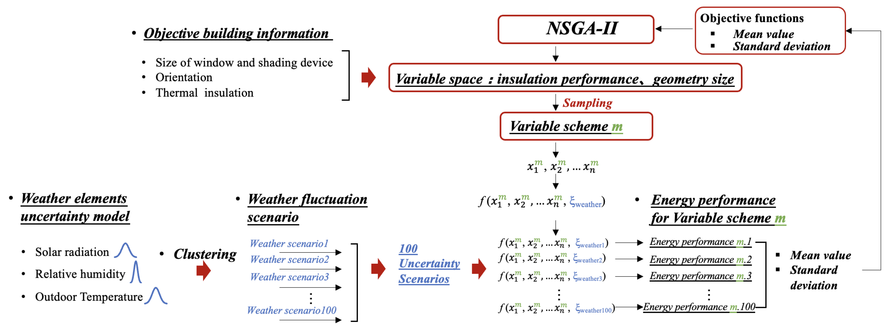
To account for the uncertainty fluctuations in weather conditions, during the optimization process, the robust optimization framework consists of three parts. First, probability distribution models are established for weather elements to describe uncertainties, and then the probability distribution model is sampled to establish weather uncertainty scenarios for the subsequent optimization process. Finally, building variables and uncertainty scenarios are input into the optimizer for robust optimization of building energy consumption performance.

Neural networks were used to construct distribution models of weather uncertainty fluctuations for subsequent optimization sampling, as described in Section 2.1. As this study focuses on the optimization of annual energy consumption fluctuations, the neural network produces a probabilistic model of the present weather elements instead of predicting the future in the context of the accumulation of forecast errors.

Sampling based on the aforementioned probability model was necessary to evaluate each building scheme in the optimization stage. However, multitarget optimization based on sampling usually leads to an unaffordable computational load. Moreover, traditional sampling methods are disadvantageous owing to their randomness. Thus, this study proposes the use of clustering algorithms instead of traditional sampling methods, as described in Section 2.2.

In the robust optimization stage, NSGA II was used as the optimizer to realize optimization. The optimization objectives are defined as the average energy consumption and the standard deviation of energy consumption of each building scheme in the face of various weather conditions from clustering to simultaneously optimize the stability of the average energy consumption and energy consumption performance in the face of weather fluctuations, as described in Section 2.3.

2.1. Uncertainty of Weather Conditions

The uncertainty of weather conditions is generated based on two neural networks. The dual-stage attention-based recurrent neural network (DARNN) [15] is used to predict the value of weather elements with weather elements as features, and the importance of weather elements to the air-conditioning load is explained through the prediction process based on the characteristic of attention mechanism. During the training process of the Bayesian recurrent neural network (Bayesian-RNN) [16], the weights and bias are established as a normal distribution based on the training set to realize the establishment of a normal distribution model of the forecast target. Therefore, weather elements are taken as prediction targets to establish their uncertainty models.

2.1.1. Dataset for Neural Networks

This section describes the two datasets used to generate the probabilistic model of weather uncertainty: a dataset of weather conditions and a dataset of building energy consumption. For the DARNN, due to the importance of calculating weather elements for computing air-conditioning energy consumption, the dataset is composed of weather data as a feature and the air-conditioning energy consumption as a label. For the Bayesian-RNN, the dataset only contains weather data, and, based on the importance calculation results from the DARNN, non-important weather elements are used as features, while important weather elements are used as labels.

The climate of Toyama Prefecture is characterized by cold and heavy snow in winter and heat and humidity in summer; it is a typical rainy and snowy area in Japan.

The weather condition dataset comes from the meteorology of Toyama Prefecture collected by the Japan Meteorological Agency [17], which is the hourly measurement data from 2019 and 2020, including elements of sea level pressure (hPa), station pressure (hPa), precipitation (mm), outdoor temperature (°C), global horizontal radiation (MJ/m${}^2$), dew temperature (°C), vapor pressure (hPa), relative humidity (%), wind speed (m/s), and cloud cover.

The dataset of building air-conditioning energy consumption is the annual energy consumption calculated based on the weather data for 2019 and 2020 using EnergyPlus [18]. This is in reference to the simulation settings in Section 2.

Furthermore, the dataset summary of the two neural networks is presented in

Table 1. Summary of training and testing datasets for neural networks.

	Training Data	Test Data
DARNN	2019/01–12 weather data and energy consumption	2020/07 and 12 energy consumption
Bayesian-RNN	2019/01–12 weather data	2020/01–12 weather data (solar radiation, relative humidity, outdoor temperature)

.

2.1.2. Importance Interpretation of Weather Elements

In this study, the dual-stage attention mechanism of the DARNN is employed to calculate the importance of weather elements for air-conditioning energy consumption. The main function of the attention mechanism [19] is to introduce the neural network to calculate the contribution weight of the encoder to the decoder. An ordinary attention usually requires three values, namely the query tensor Q, the key tensor K, and the value tensor V, as shown in Equation (1). The attention score is calculated as the importance of the input value to the prediction target, as shown in Equation (2).

$$\begin{array}{cc}\hfill & Q=W_{q}Q\hfill \\ \hfill & K=W_{k}K\hfill \\ \hfill & V=W_{v}V\hfill \end{array}$$

(1)

where $W_q$, $W_k$, $W_v$ means weights matrix.

$$\begin{array}{c}A=K^{T}Q\\ A^{\prime }=softmax\left(A\right)\end{array}$$

(2)

The DARNN consists of two parts: the encoder and the decoder. Both stages use the attention mechanism and involve several steps, including calculating attention scores, computing attention weights, updating inputs or calculating CoVe (contextualized vector), and computing hidden states. Therefore, in the calculation process of the attention score and weight, the important results for the weather elements are obtained. The specific description and adoption of rationality for the importance interpretation of the DARNN were proven in a previous study by the author of [20]. The details of hyperparameters are shown in

Table 2. Hyperparameter of DARNN.

Hyperparameter	Encoder	Decoder
Learning rate	0.001	0.001
Batch size	64	64
Hidden size	128	256
Num_layers	2	2
Sequence length	24	24

.

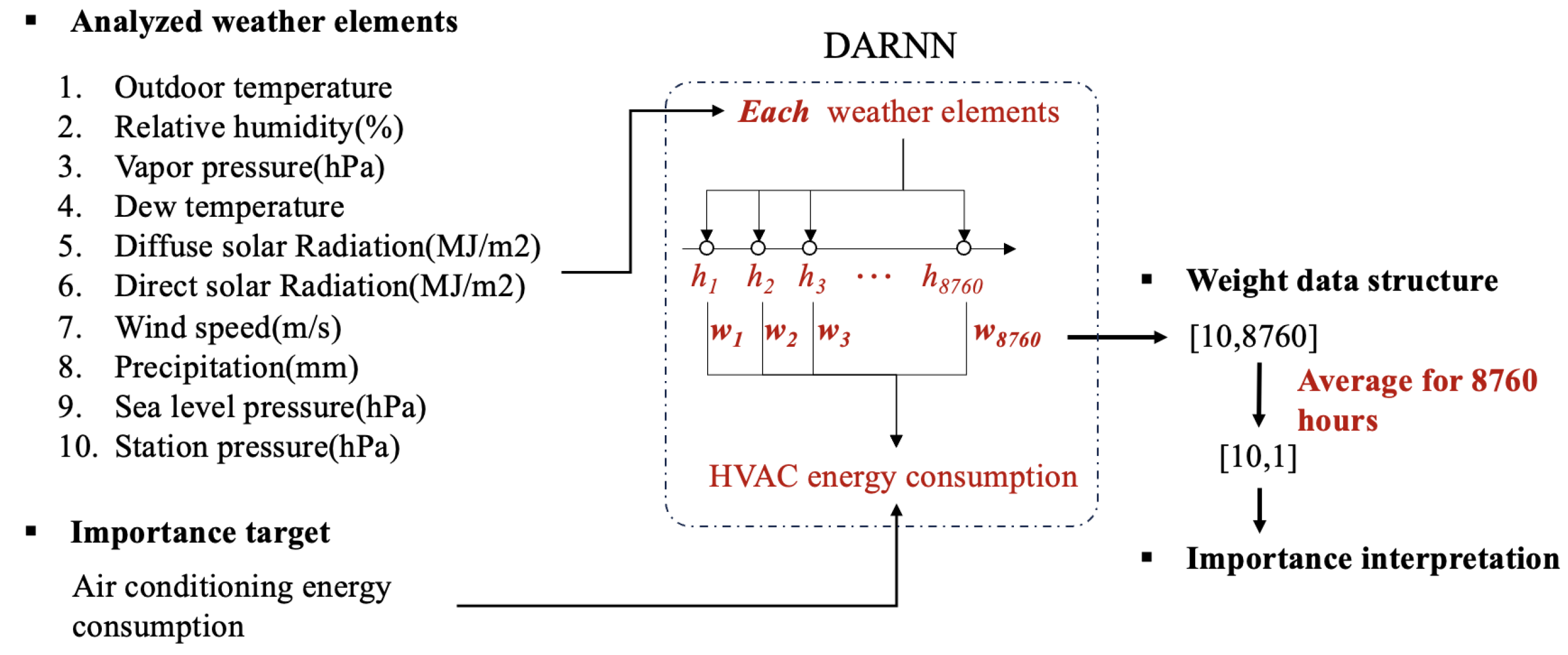
Figure 1 provides an overview of the process of using the DARNN to predict the air-conditioning energy consumption based on weather elements. The attention mechanism in the neural network calculates the weights for each weather element with respect to the target prediction. Since a total of 10 weather elements are considered, each with a time span of one year (8760 h), the resulting weight data structure is [10, 8760]. To facilitate statistical analysis, the weight data structure is transformed into [10, 1] by taking the average along the time dimension, serving as the final outcome of importance interpretation.

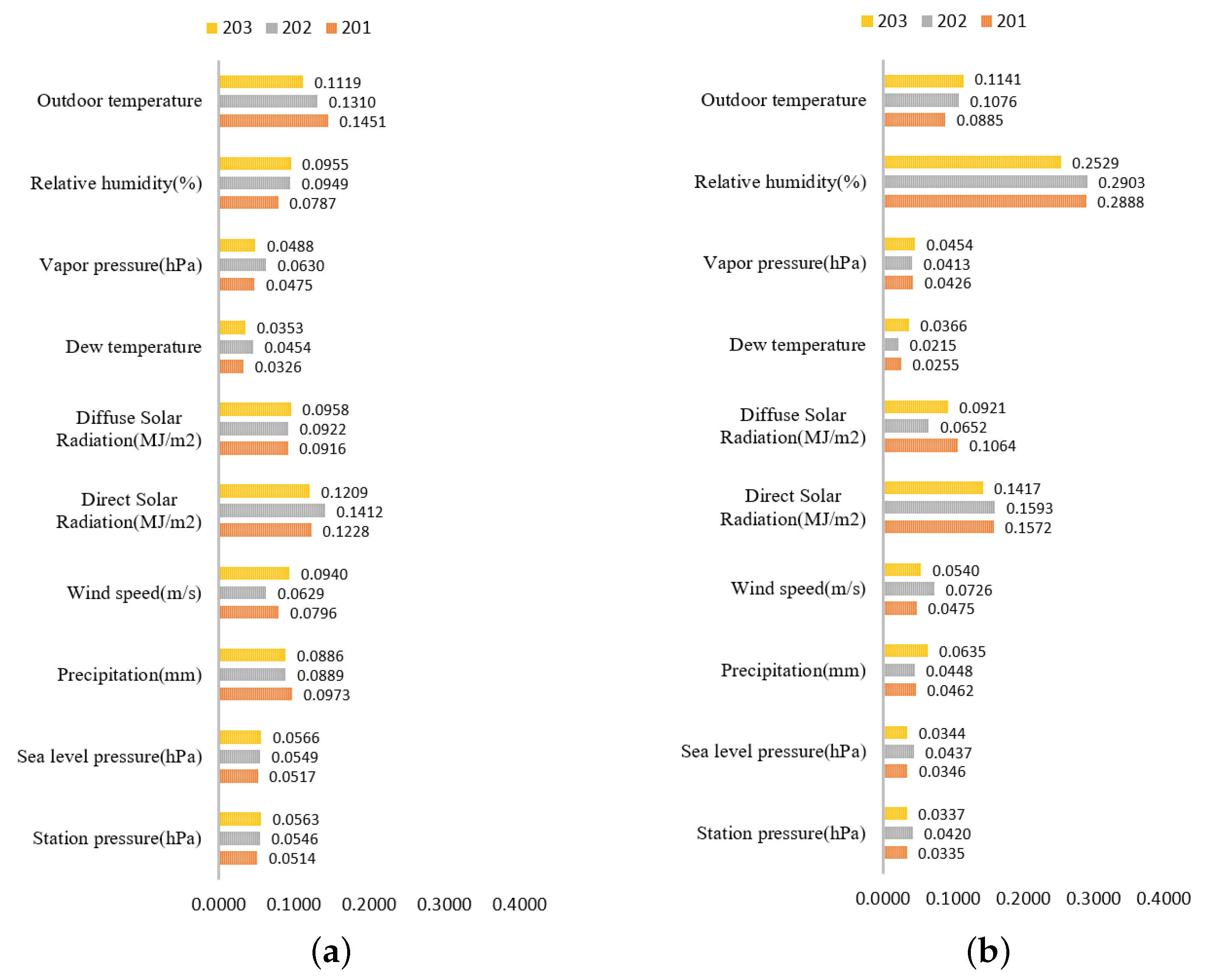
Taking three units on the middle floor of the building as representatives, namely, units 201, 202, and 203, and considering the importance of weather elements to the air-conditioning energy consumption in winter and summer, the importance interpretation results of the DARNN are shown in Figure 2. The 2019 dataset was used as the training set for the DARNN, and the July and December 2020 datasets were used as the test set. The results show that in both winter (December) and summer (August), the three most important factors were solar radiation, outdoor temperature, and relative humidity.

2.1.3. Uncertainty Modeling for Weather Elements

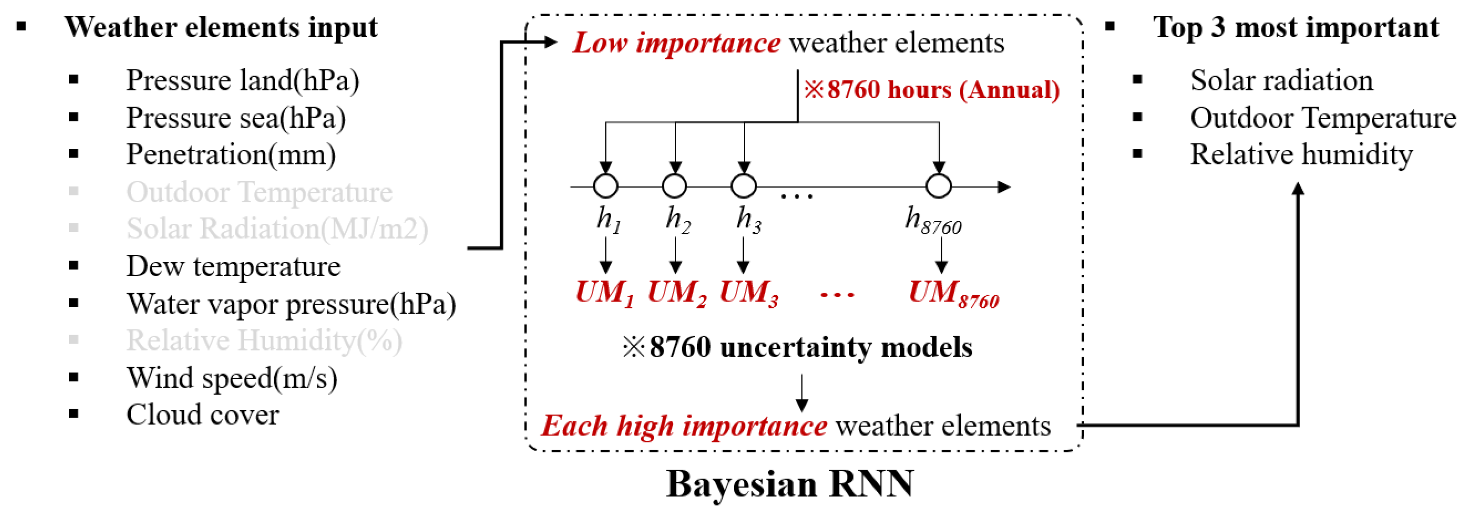
Based on the importance interpretation results, solar radiation, relative humidity, and outdoor temperature were used as uncertainty modeling objects. As there are latent correlations between weather elements, weather elements other than those mentioned above are used as input values for the Bayesian-RNN, and the outputs are the uncertainty models of the object weather elements, as shown in Figure 3, and the details of the hyperparameters are shown in Table 3. The result of uncertainty modeling was that 8760 normal distribution models were established for each element, that is, one normal distribution model at each hour of the year, to reflect the change in weather elements over time. The predictive accuracy and underlying principles of the Bayesian-RNN for weather uncertainty have been validated in the paper [20].

Figure 3. Framework of uncertainty modeling.

Figure 3. Framework of uncertainty modeling.

Where UM${}_n$ means uncertainty model.

Table 3. Hyperparameter of Bayesian-RNN.

Hyperparameter	Value
Learning rate	0.0001
Batch size	256
Hidden size	128
Num_layers	2 (BayesianLSTM layter, Linear layer)
Sequence length	24

Table 3. Hyperparameter of Bayesian-RNN.

Hyperparameter	Value
Learning rate	0.0001
Batch size	256
Hidden size	128
Num_layers	2 (BayesianLSTM layter, Linear layer)
Sequence length	24

To verify the reliability of the generated uncertainty model for three weather elements, this study sampled 3000 sets of data based on the normal distribution model of each hour and compared the mean value of the sampled data with the measurement data using the mean average percentage error (MAPE) as an indicator during winter (December) and summer (August), as shown in

Table 4. MAPE of uncertainty models for three weather elements.

	Winter (December)	Summer (August)
Outdoor temperature	9.50%	2.60%
Relative humidity	3.90%	4.20%
Solar radiation	13.00%	9.10%

.

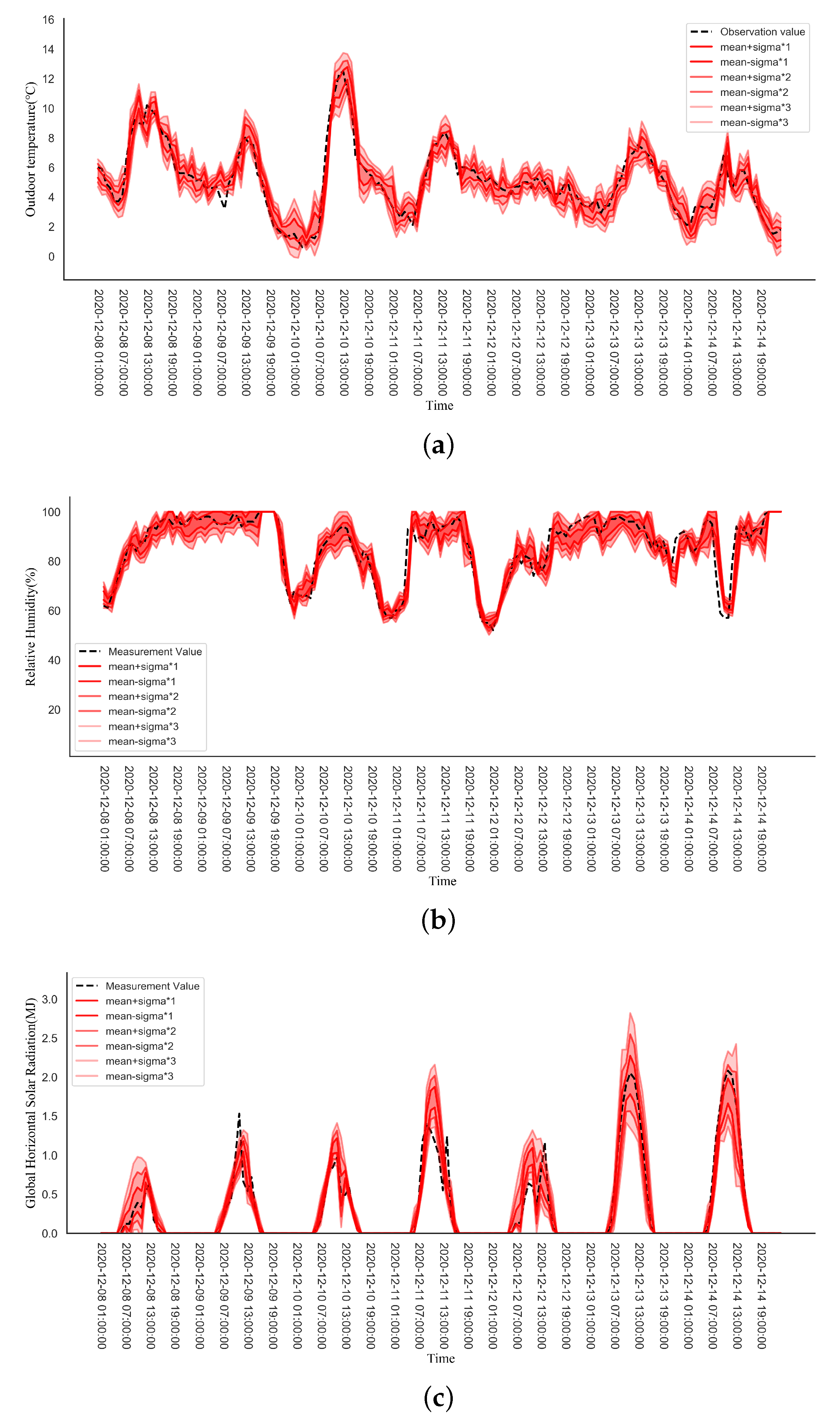
Taking the second week of December as an example, the line chart describes the uncertainty modeling results of the three weather elements, and the different red concentrations in the chart represent the mean plus or minus n times (n = 1, 2, 3) standard deviation, as shown in Figure 4.

2.2. Sampling by Clustering Algorithm

Sampling based on the uncertainty model described above is required to account for uncertainty in the subsequent optimization process. However, traditional sampling methods, such as the Monte Carlo sampling method, usually have difficulty ensuring the representativeness of the sampling results in the sample space when extracting a small number of sample results. Although increasing the number of samples can solve this problem, the calculation load of the subsequent process increases significantly. Thus, this study used the k-means algorithm [21] to obtain the cluster center as the final sampling result. Although the clustering algorithm is a type of classification technique, its clustering principle ensures that the representativeness of the clustering is centered in the entire sample space; i.e., the clustering centers are included in the sampling space and evenly distributed. Thus, the cluster centers are used as the sampling results.

2.2.1. Comparison between Clustering Algorithm and Traditional Sampling Methods

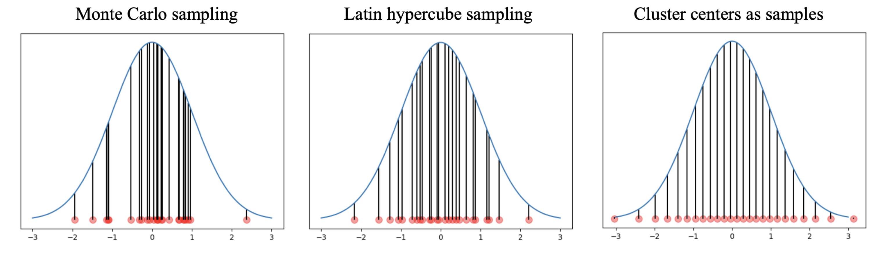
The Monte Carlo and Latin hypercube samplings are commonly used traditional sampling methods. However, due to the reliance on randomness in the sampling process, there are instances where the representativeness of the sampling results cannot be guaranteed. In this study, these two methods are used as benchmarks for comparing the sampling effectiveness of clustering algorithms. As the sampling objects in this study are multiple normal distributions, to compare the representativeness of the sampling results in the sample space between the clustering algorithm and the traditional sampling method with a small number of samples, the standard normal distribution with a mean of 0 and a standard deviation of 1 was sampled 25 times using the Monte Carlo method and the Latin hypercube method. In addition, for the same normal distribution, 100,000 samples were first randomly selected, and, thereafter, the samples were clustered using the k-means algorithm to obtain 25 cluster centers as 25 samples, as shown in Figure 5.

The results show that the sampling results of both the Monte Carlo and Latin hypercube sampling methods have varying degrees of sample concentration, which leads to a lack of representativeness for some normal distributions, especially at the edges. In contrast, the clustering centers as the sampling results effectively solve the above problem, which is uniformly distributed in the normal distribution space based on probability, and the edges are effectively sampled.

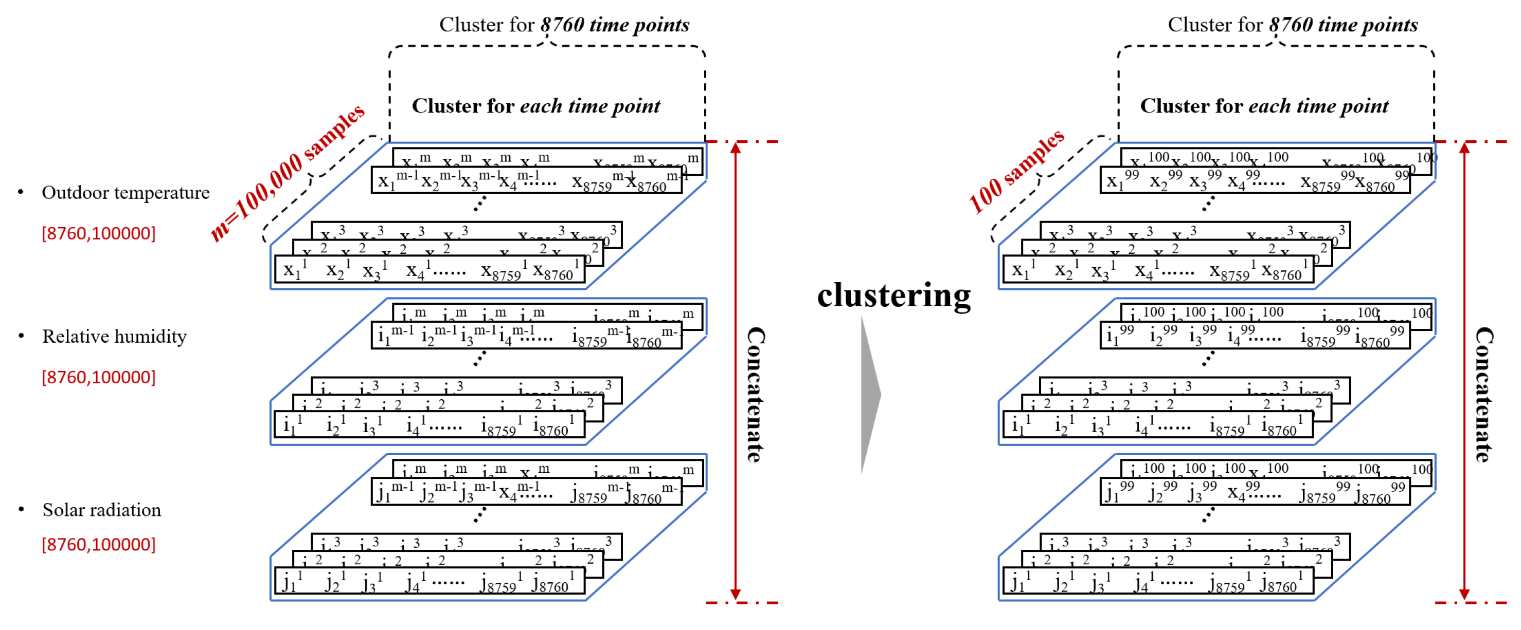
2.2.2. Clustering for Establishment of Uncertainty Scenarios for Weather Elements

Each weather element was sampled 100,000 times based on the normal distribution at each hour; thus, the sampling data results with the structure [8760, 100,000] were obtained. As there are three weather elements, the final data structure obtained through the sampling process is [3, 8760, 100,000]. The dimension of the number of samples was clustered to obtain 100 cluster centers due to which the data structure became [3, 8760, 100], as shown in Figure 6. Thus, there were 100 clustering centers as samples at each hour of the three weather elements.

2.3. Robust Optimization

The proposed robust optimization framework in this study differs from traditional optimization approaches in that it introduces uncertainty into the optimization process to realize that the results of each scheme are range values. The mean value and standard deviation of the range are used as the optimization objective functions. The inputs, outputs, and optimization flow of the robust optimization framework are described in this section.

The input side of robust optimization contains two components, variables, and uncertainty scenarios, both of which affect the building energy consumption, as described in Section 2.3.1.

Two optimization objectives are included: the average value and the standard deviation of building air-conditioning consumption for each building scheme in the face of various weather uncertainty scenarios to represent the average performance and fluctuation, as described in Section 2.3.2.

Section 2.3.3 describes the optimizer used in this study during the optimization process and the order in which the variables and uncertainties participate in the calculation of the optimization objectives.

2.3.1. Variables and Uncertainty of Robust Optimization

The optimization variables considered in this study are defined as building elements that can be determined by engineers and designers during the design phase. The variables came from three fields, the geometric information of windows and shading devices, building orientation, and thermal insulation performance, a total of 25 elements.

Table 5. Characterization of optimization variables.

NO.	Optimization Variables	Range/Value	Accuracy
X1	South window height [m]	[1.7, 2.2]	0.05
X2	South window width [m]	[1.0, 5.8]	0.05
X3	East window height [m]	[0.5, 2.0]	0.05
X4	East window width [m]	[0.9, 5.5]	0.05
X5	West window height [m]	[0.5, 2.0]	0.05
X6	West window width [m]	[0.9, 5.5]	0.05
X7	South shading device width [m]	[0.1, 3.0]	0.01
X8	Building orientation [°]	[−90, 90]	0.1
X9	External wall thermal insulation [-]	G2, G1, H25, H4
X10	Internal wall thermal insulation [-]	G2, G1, H25, H4
X11–X19	South window thermal insulation [-]	G2, G1, H25, H4
X20–X22	East window thermal insulation [-]	G2, G1, H25, H4
X23–X25	West window thermal insulation [-]	G2, G1, H25, H4

shows the range of variation in each element in the case building, and more detailed building information will be introduced in Section 3. These variables are discrete variables, and the value accuracy of each variable is indicated by “Accuracy” in the table. In addition, X9 through X25 are variables of thermal insulation performance, and the range of values is the four thermal insulation performance standards mentioned in Section 3.3, which do not involve value accuracy.

The clustering results in Section 2.2 are used as inputs for the robust optimization of weather uncertainty scenarios. During the optimization process, the optimizer randomly generates building schemes based on variables and, thereafter, uses simulation software to calculate the energy consumption performance of each scheme under various weather uncertainty scenarios.

2.3.2. Objectives of Robust Optimization

Building energy performance is affected by both building variables and weather uncertainties, as shown in Equation (3), so the energy consumption result of each building scheme generated from variable space is a dataset rather than a fixed value.

$$\mathrm{Building}\mathrm{energy}\mathrm{performance}=f\left(x_1^m,x_2^m,\dots x_{25}^m,{\xi }_{\mathrm{weather}}\right)$$

(3)

where x denotes the optimization variables, $x^m$ denotes the mth set of building schemes selected from the variable space, $x_{1\dots 25}$ denotes each variable in the mth building scheme (such as the building orientation and window size), and $\xi$ indicates the weather uncertainty scenarios generated in Section 3.2.

To ensure the robustness of the optimization results, the optimization objective was divided into two parts: the average value of the results dataset was used as the average performance evaluation index in the face of uncertainty scenarios, and the standard deviation was the evaluation index of the fluctuation range, as shown in Equations (4) and (5).

$$\mathrm{Objective}\mathrm{function}\mathrm{Avg}=\mathrm{Avg}.\left(\begin{array}{c}f\left(x_1^m,x_2^m,\dots x_n^m,{\xi }_{\mathrm{weather}1}\right)\\ f\left(x_1^m,x_2^m,\dots x_n^m,{\xi }_{\mathrm{weather}2}\right)\\ ⋮\\ f\left(x_1^m,x_2^m,\dots x_n^m,{\xi }_{\mathrm{weather}j}\right)\end{array}\right)$$

(4)

$$\mathrm{Objective}\mathrm{function}\mathrm{Std}\mathrm{Dev}=StdDev.\left(\begin{array}{c}f\left(x_1^m,x_2^m,\dots x_n^m,{\xi }_{\mathrm{weather}1}\right)\\ f\left(x_1^m,x_2^m,\dots x_n^m,{\xi }_{\mathrm{weather}2}\right)\\ ⋮\\ f\left(x_1^m,x_2^m,\dots x_n^m,{\xi }_{\mathrm{weather}j}\right)\end{array}\right)$$

(5)

where ${\xi }_{weather1\dots j}$ represents multiweather uncertainty scenarios.

Thus, considering that there are two air-conditioned rooms in each unit, namely, the LDK and bedroom, a situation in which the optimization is difficult to converge because of too many optimization objectives when each household is optimized individually has been avoided. Four optimization objectives are defined in terms of air-conditioning energy consumption in buildings:

• The average of the total energy consumption in the LDK room facing uncertainty scenarios.
• The standard deviation of the total energy consumption in the LDK room facing uncertainty scenarios.
• The average of the total energy consumption in the bedroom facing uncertainty scenarios.
• The standard deviation of the total energy consumption in the bedroom facing uncertainty scenarios.

2.3.3. Robust Optimization Flow

NSGA-II [22] was used as the optimizer; its configuration is shown in

Table 6. Configurations of NSGA-II.

Settings and Operator	Method/Value
Max generation	100
Population size	40
Offspring size	10
Sampling	Lartin hypercube
Selection	Tournament
Mutation	Polynomial Mutation (0.1)
Crossover	Simulated Binary Crossover (0.5)

. In the optimization process, a set of variable values is extracted by the optimizer from the variable space to generate a design scheme, and the air-conditioning energy consumption of the scheme is calculated under various uncertainty scenarios based on EnergyPlus. The mean and standard deviation of the energy performance of each design scheme were returned to the optimizer to calculate the fitness, and the above process was repeated, as shown in Figure 7.

Compared with traditional optimization results, the optimization flow proposed in this study produces an optimal energy consumption distribution probability model rather than an optimal fixed energy consumption value. In the design stage, it can more comprehensively describe the fluctuation of building energy consumption in the face of weather uncertainty and help decision-makers make more accurate decisions.

3. Case Study and Simulation Settings

3.1. Geometry of Typical Residential Building

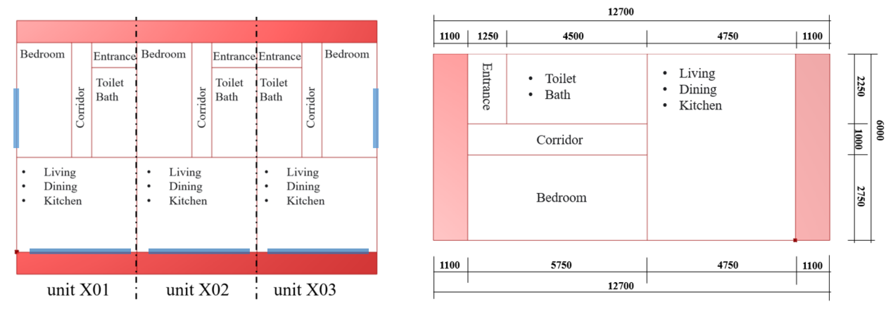
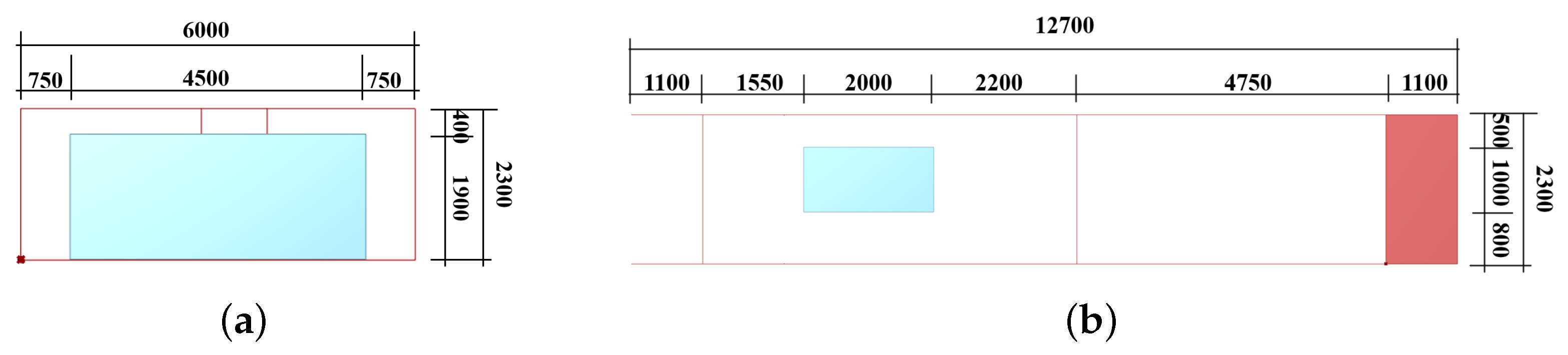
In this study, an LDK south-facing three-story MUH with three units on each floor has been considered. One LDK (living room, dining, and kitchen), bedroom, toilet, entrance with a corridor in each unit, plan of each floor, and size of each unit are shown in Figure 8. All units have exterior windows on the south wall of the LDK and on the bedroom walls of the east- and west-side units; the facade size of the unit is shown in Figure 9, with the west unit as an example.

3.2. Simulation Settings

In this study, the mathematical modeling of weather uncertainties, described in Section 2, and the resulting fluctuations in the energy consumption results were focused on during the design phase, and ideal fixed values were used for other simulation settings. The details of the fixed simulation settings are listed in

Table 7. Simulation settings.

Air-Conditioning Room	LDK Bedroom
Cooling period	July-September
Heating period	December-March
Cooling/Heating Setpoint	27 °C (28 °C during night)/20 °C
Family Stucture	The couple(two people)
Infiltration rate	0.5 ACH (Energy recovery efficiency 70%)

(refers to [23]). Only the LDK and bedroom were air-conditioned rooms, and the family composition was envisaged as a couple. Assuming that the infiltration frequency was 0.5/h and the enthalpy efficiency of the total heat exchanger was 70%, the ventilation frequency was set to 0.15 times.

3.3. Thermal Insulation Performance

Four thermal insulation performance standards were considered in this study: the Japan 1992 energy-saving standard (H4), the Japan 2013 energy-saving standard (H25), the HEAT20 G1 housing exodermis insulation standard (G1), and the HEAT20 G2 housing exodermis insulation standard (G2) [24]. These four thermal insulation performance standards also represent the thermal insulation performance of different grades of building envelopes in Japan and serve as a benchmark for comparing the optimization results of this study. The U values set for each thermal insulation standard for buildings in the seven climate zones of Japan are listed in

Table 8. Thermal insulation performance standard of H4.

	Area 1	Area 2	Area 3	Area 4	Area 5	Area 6	Area 7
External wall (W/m${}^2$·K)	0.9	0.9	2.4	2.7	3	3	3.2
External ceiling (W/m${}^2$·K)	0.42	0.42	1.05	1.12	1.55	1.55	2.3
Window (W/m${}^2$·K)	2.91	2.91	2.91	2.91	4.65	4.65	4.65
External floor (W/m${}^2$·K)	0.9	0.9	2.0	2.1	2.9	2.9	4
Internal wall (W/m${}^2$·K)	3.04	3.04	3.04	3.04	3.04	3.04	3.04
Internal ceiling/floor (W/m${}^2$·K)	2.79	2.79	2.79	2.79	2.79	2.79	2.79

,

Table 9. Thermal insulation performance standard of H25.

	Area 1	Area 2	Area 3	Area 4	Area 5	Area 6	Area 7
External wall (W/m${}^2$·K)	0.7	0.7	0.9	0.9	1.3	1.3	1.3
External ceiling (W/m${}^2$·K)	0.27	0.27	0.35	0.35	0.35	0.35	0.35
Window (W/m${}^2$·K)	2.33	2.33	2.33	2.33	4.65	4.65	4.65
External floor (W/m${}^2$·K)	0.65	0.65	0.8	0.8	1	1	1
Internal wall (W/m${}^2$·K)	2.333	2.333	2.333	2.333	2.333	2.333	2.333
Internal ceiling/floor (W/m${}^2$·K)	2.079	2.079	2.079	2.079	2.079	2.079	2.079

,

Table 10. Thermal insulation performance standard of G1.

	Area 1	Area 2	Area 3	Area 4	Area 5	Area 6	Area 7
External wall (W/m${}^2$·K)	0.65	0.65	0.7	0.75	0.75	0.98	0.98
External ceiling (W/m${}^2$·K)	0.23	0.23	0.25	0.25	0.25	0.3	0.3
Window (W/m${}^2$·K)	1.6	1.6	1.9	1.9	1.9	2.33	2.33
External floor (W/m${}^2$·K)	0.54	0.54	0.6	0.6	0.6	0.75	0.75
Internal wall (W/m${}^2$·K)	1.406	1.406	2.333	2.333	2.333	2.333	2.333
Internal ceiling/floor (W/m${}^2$·K)	2.079	2.079	2.079	2.079	2.079	2.079	2.079

and

Table 11. Thermal insulation performance standard of G2.

	Area 1	Area 2	Area 3	Area 4	Area 5	Area 6	Area 7
External wall (W/m${}^2$·K)	0.5	0.5	0.5	0.35	0.35	0.7	0.7
External ceiling (W/m${}^2$·K)	0.24	0.24	0.24	0.19	0.19	0.24	0.24
Window (W/m${}^2$·K)	1.3	1.3	1.3	1.3	1.3	1.9	1.9
External floor (W/m${}^2$·K)	0.5	0.5	0.5	0.26	0.26	0.58	0.58
Internal wall (W/m${}^2$·K)	1.153	1.153	1.153	2.333	2.333	2.333	2.333
Internal ceiling/floor (W/m${}^2$·K)	1.609	1.609	1.609	2.079	2.079	2.079	2.079

. The building in question in Toyama Prefecture is located in the fifth climate zone. Thus, the energy consumption of the building, along with the thermal insulation performance of the fifth climate zone, was used as a benchmark for the optimization results.

4. Results

4.1. Building Information after Optimization

Through optimization, a series of optimal solutions were selected as examples to illustrate the optimization results.

Before optimization, the thermal insulation performance of the fifth zone of the four thermal insulation standards described in Section 3 was used in the case study building. The optimal thermal insulation performance for each part of the building is listed in

Table 12. Thermal insulation of wall after optimization.

	Thermal Transmittance (W/m${}^2$·K)	Thermal Insulation Standard and Climate Area
External wall	0.35	G2 5th zone
Roof	0.19	G2 5th zone
Floor	0.26	G2 5th zone
Internal floor/ceiling	2.709	G2 5th zone
Internal wall	1.153	G2 3th zone

. As the excessive thermal insulation performance of the external wall leads to an additional cooling load, the thermal insulation of the external wall of the optimization result is the fifth area of the G2 standard. However, the optimization results emphasize the importance of the thermal insulation performance of internal walls to reduce the heating and cooling caused by the temperature difference between adjacent rooms or units due to the difference in unit location and ratio to exterior walls. The thermal insulation performance of the third area, which was selected as the thermal insulation of the internal walls, was superior to that of the fifth area.

The optimal window sizes are listed in

Table 13. Size of window after optimization.

	Height (m)	Width (m)
South window (LDK)	1.75	1.97
West window (Bedroom)	0.64	0.9
East window (Bedroom)	0.67	2.34

. Compared to the original situation, the south window area becomes 45.3%, the west window area becomes 54%, and the east window area becomes 73.5%. As the thermal insulation performance of each window was optimized independently, the optimization results for the thermal insulation performance of the window are shown in

Table 14. Thermal insulation of south window after optimization.

Thermal Transmittance (W/m${}^2$·K)
	Unit No.	×01	×02	×03
South window	10×	1.3	1.3	1.6
	20×	1.3	1.9	1.3
	30×	1.3	1.9	1.3

,

Table 15. Thermal insulation of east window after optimization.

Thermal Transmittance (W/m${}^2$·K)
	103	203	303
East window	2.33	1.9	1.3

and

Table 16. Thermal insulation of west window after optimization.

Thermal Transmittance (W/m${}^2$·K)
	101	201	301
West window	1.3	1.3	1.6

. Compared with the original thermal insulation performance of 1.3 W/m${}^2$·K for all windows, some windows in the optimization results remained unchanged, and some windows declined to a certain extent.

In addition, the building orientation was optimized from south to 18.5${}^{\circ }$ southwest, and the depth of the southern shading devices was optimized from 1.1 m to 1.53 m.

4.2. Comparison of Energy Consumption before and after Robust Optimization

This section presents the improvement in the robustness of the building energy performance before and after optimization when considering weather uncertainty scenarios. The optimal scheme selected from the optimization results is the most effective for robust optimization. For the convenience of statistical analysis and visualization of optimization results for multiple objectives, the average energy consumption of the LDK and the bedroom are combined into the average energy consumption of the entire building, while the standard deviations of the LDK and bedroom are merged into the standard deviation of the overall energy consumption of the entire building.

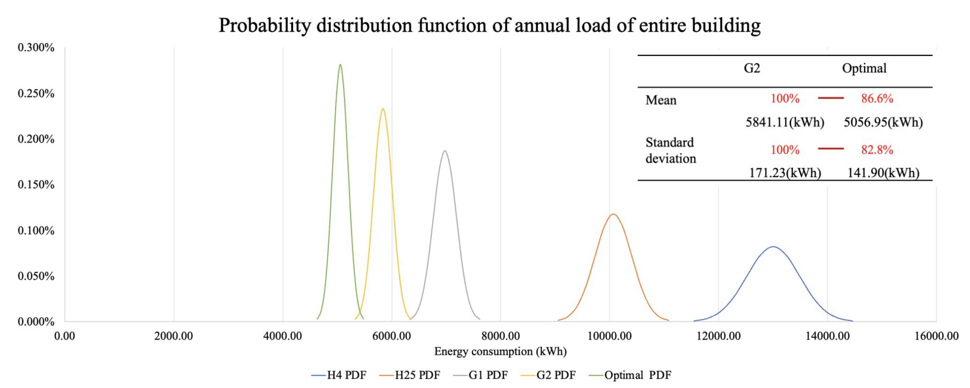
One hundred weather uncertainty scenarios were generated as described in Section 2.2.2; thus, there were 100 energy performance results for each design scheme. Figure 10 shows the air-conditioning energy consumption results of an entire building for thermal insulation standards H4, H25, G1, and G2 (5th climate zone) and the optimal scheme, i.e., the probability distribution function (PDF) curve generated based on the mean and standard deviation of 100 results. For the four thermal insulation standards on the display, G2 had the ideal mean and standard deviation, that is, the lowest mean and smallest standard deviation.

Compared with the thermal insulation standard of G2, the thermal insulation performance of the external wall in the optimal scheme of this study almost no change. However, the thermal insulation performance of the internal wall is improved, and the building geometry information (windows and shading device size, building orientation) is adjusted.

Usually, due to the influence of location and floor, there is a significant difference in the indoor environment among different units, which leads to heat transfer between adjacent units or rooms except for the outdoor environment. When considering the uncertainty of weather conditions, the heat transfer between adjacent units becomes even more complex, exacerbating fluctuations in energy consumption for units. The optimization results reduce the heat transfer between adjacent units by improving the insulation performance of the inner wall, thereby improving the average energy consumption performance and reducing the fluctuation of building energy consumption. In addition, by increasing the depth of shading objects, reducing the size of windows, and adjusting the orientation of buildings, the impact of solar radiation on buildings is effectively reduced. Therefore, even in the face of the same uncertainty of solar radiation, the optimization results have a more stable performance of energy consumption.

For the optimal scheme, the average energy consumption decreased by 13.4% compared with that of G2, and the standard deviation decreased by approximately 17.2%. In other words, in the face of uncertainty, the optimal scheme proposed in this study has lower average energy consumption results and a more stable energy consumption performance than most energy-saving standards in Japan at the current stage.

The optimization results verified that the robust optimization framework proposed in this study can effectively optimize the energy performance stability and average energy consumption of the scheme under uncertainty, thereby alleviating the gap between simulation and measurement values, and ensuring a good performance of the building during the actual use stage. At present, the majority of environmental performance evaluation systems, such as LEED [25], primarily rely on referencing the actual operational performance when assessing the energy consumption performance level of buildings, which emphasizes the importance of building energy performance in actual use. The results of this study can assist decision-makers in designing high-performance buildings that have a practical significance in actual usage, rather than solely relying on fixed simulation results.

5. Conclusions

This study combines a weather uncertainty scenario modeling method using deep learning and a highly representative sampling method using a clustering algorithm and proposes a robust optimization framework to achieve the optimization of building energy performance considering uncertainty. The optimization framework is based on the high-precision reproduction of weather element uncertainty in the simulation stage to achieve the modeling of fluctuations in air-conditioning energy consumption and improve the evaluation indices to the mean and standard deviation to ensure the ability to evaluate building energy fluctuations during the simulation stage.

The weather uncertainty scenario modeling method establishes the uncertainty fluctuations of solar radiation, relative humidity, and temperature as normal distributions for each hour of the year. The reliability of this method is demonstrated by calculating the mean absolute percentage error (MAPE) between the mean values of the normal distribution and the measurement values, which ranges from 3% to 13%.

Compared to traditional sampling methods, using the cluster center of a clustering algorithm as sampling results leads to a more uniform sample results distribution, which results in better representativeness of the overall sampling space. Moreover, for a normal distribution, the clustering algorithm does not overlook regions with lower probabilities.

Furthermore, taking the mean value and standard deviation of energy fluctuation as the optimization objectives, the optimization results show that in the face of weather uncertainty, the average energy consumption of buildings has decreased by 13.4%, and the standard deviation of energy consumption fluctuations has decreased by 17.2%. The goals of low average energy consumption and low energy fluctuation of the building were achieved, namely, the risk from uncertainty fluctuation was controlled by robust optimization.

The scientific contribution of this study is to validate the feasibility of utilizing deep learning to establish a normal distribution model for certain meteorological elements, proposing and demonstrating the feasibility and advantages of using cluster centers as sampling points and providing other researchers with a sampling alternative with low random interference. In addition, the feasibility of combining a clustering algorithm, deep learning, and robust optimization to achieve optimization considering uncertainty is also demonstrated by the uncertainty modeling results and optimization results of this study. This demonstrates that further optimization of building solutions under the premise of considering uncertainty is necessary even in the context of the current high insulation performance standards.

In the robust optimization process of this study, the standard deviation is selected as one of the optimization objectives, which effectively reduces the fluctuation range. However, there are obvious conservative phenomena in the optimization results. After optimization, although the maximum energy consumption in the fluctuation range has been significantly reduced, the minimum energy consumption value has also become larger, that is, the minimum energy consumption result has worsened. Therefore, as a future research direction, it is necessary to consider new objective functions to address the conservatism issue.

References

- Ritchie, H.; Roser, M. Urbanization. Our World in Data. 2018. Available online: https://ourworldindata.org/urbanization (accessed on 31 March 2023).
- Saidur, R.; Masjuki, H.H.; Jamaluddin, M. An application of energy and exergy analysis in residential sector of Malaysia. Energy Policy 2007, 35, 1050–1063. [Google Scholar] [CrossRef]
- National Association of Home Builders Discusses Economics and Housing Policy. 2020 Multifamily Completion Data: Property Size. Available online: https://eyeonhousing.org/2021/08/2020-multifamily-completion-data-property-size/ (accessed on 8 June 2023).
- BC Housing. 2018 BC Residential Building Statistics and Trends Report; BC Housing: Vancouver, BC, Canada, 2018; p. 61.
- Statistics Bureau, Ministry of Internal Affairs and Communications. 2018 Housing and Land Statistics Survey. Available online: https://www.stat.go.jp/data/jyutaku/2018/pdf/g_gaiyou.pdf (accessed on 28 May 2023).
- Wu, W.; Skye, H.M. Residential net-zero energy buildings: Review and perspective. Renew. Sustain. Energy Rev. 2021, 142, 110859. [Google Scholar]
- De Wilde, P. The gap between predicted and measured energy performance of buildings: A framework for investigation. Autom. Constr. 2014, 41, 40–49. [Google Scholar] [CrossRef]
- Shi, X.; Si, B.; Zhao, J.; Tian, Z.; Wang, C.; Jin, X.; Zhou, X. Magnitude, causes, and solutions of the performance gap of buildings: A review. Sustainability 2019, 11, 937. [Google Scholar] [CrossRef] [Green Version]
- Bhandari, M.; Shrestha, S.; New, J. Evaluation of weather datasets for building energy simulation. Energy Build. 2012, 49, 109–118. [Google Scholar] [CrossRef]
- Sun, Y.; Gu, L.; Wu, C.J.; Augenbroe, G. Exploring HVAC system sizing under uncertainty. Energy Build. 2014, 81, 243–252. [Google Scholar] [CrossRef]
- Wang, L.; Mathew, P.; Pang, X. Uncertainties in energy consumption introduced by building operations and weather for a medium-size office building. Energy Build. 2012, 53, 152–158. [Google Scholar] [CrossRef] [Green Version]
- Sun, Y.; Heo, Y.; Tan, M.; Xie, H.; Jeff Wu, C.; Augenbroe, G. Uncertainty quantification of microclimate variables in building energy models. J. Build. Perform. Simul. 2014, 7, 17–32. [Google Scholar] [CrossRef]
- Luo, Z.; Lu, Y.; Cang, Y.; Yang, L. Study on dual-objective optimization method of life cycle energy consumption and economy of office building based on HypE genetic algorithm. Energy Build. 2022, 256, 111749. [Google Scholar] [CrossRef]
- Imran; Iqbal, N.; Kim, D.H. IoT Task Management Mechanism Based on Predictive Optimization for Efficient Energy Consumption in Smart Residential Buildings. Energy Build. 2022, 257, 111762. [Google Scholar] [CrossRef]
- Qin, Y.; Song, D.; Chen, H.; Cheng, W.; Jiang, G.; Cottrell, G. A dual-stage attention-based recurrent neural network for time series prediction. arXiv 2017, arXiv:1704.02971. [Google Scholar]
- Blundell, C.; Cornebise, J.; Kavukcuoglu, K.; Wierstra, D. Weight uncertainty in neural networks. In Proceedings of the 32nd International Conference on Machine Learning, Lille, France, 6–11 July 2015; Volume 2, pp. 1613–1622. [Google Scholar]
- Japan Meterological Agency. Search Past Weather Data, Toyama Prefecture Toyama. 2021. Available online: https://www.data.jma.go.jp/obd/stats/etrn/index.php?prec_no=55&block_no=47607&year=2021&month=1&day=1&view= (accessed on 9 March 2020).
- National Renewable Energy Laboratory. EnergyPlus. 2021. Available online: https://energyplus.net/ (accessed on 18 April 2022).
- Bahdanau, D.; Cho, K.; Bengio, Y. Neural machine translation by jointly learning to align and translate. arXiv 2014, arXiv:1409.0473. [Google Scholar]
- Wang, J.; Mae, M.; Taniguchi, K. Uncertainty modeling method of weather elements based on deep learning for robust solar energy generation of building. Energy Build. 2022, 266, 112115. [Google Scholar] [CrossRef]
- MacQueen, J. Some methods for classification and analysis of multivariate observations. In Proceedings of the Fifth Berkeley Symposium on Mathematical Statistics and Probability, Oakland, CA, USA, 1 January 1967; Volume 1, pp. 281–297. [Google Scholar]
- Deb, K.; Pratap, A.; Agarwal, S.; Meyarivan, T. A fast and elitist multiobjective genetic algorithm: NSGA-II. IEEE Trans. Evol. Comput. 2002, 6, 182–197. [Google Scholar] [CrossRef] [Green Version]
- Institute for Built Environment and Carbon Neutral for SDGs. Explanation of Energy Consumption Calculation Method in the Criteria of Judgment of Housing Business Builder. 2012. Available online: http://www.heat20.jp/grade/index.html (accessed on 31 March 2023).
- Insulation Technology Development Committee for Housing with an Eye on 2020, H. Investigation Committee of Hyper Enhanced Insulation and Advanced Technique for 2020 Houses Design Guide Plus. 2020, pp. 124–125. Available online: https://www.ibec.or.jp/ee_standard/build_standard.html (accessed on 31 March 2023).
- U.S. Green Building Council. LEED Rating System. 2023. Available online: https://www.usgbc.org/leed (accessed on 9 June 2023).
Figure 1.
Framework of importance interpretation of weather elements.
Figure 2.
Importance ranking of weather elements to energy consumption. (a) Importance ranking of weather elements to energy consumption in winter; (b) importance ranking of weather elements to energy consumption in summer.
Figure 4.
Description of the prediction distribution for three weather elements. (a) Description of the prediction distribution of outdoor tmperature in winter; (b) Description of the prediction distribution of relative humidity in winter; (c) Description of the prediction distribution of solar radiation in winter.
Figure 5.
Comparison of clustering results with traditional sampling methods.
Figure 6.
Date structure of clustering result.