Experimental Behavior and Modelling of Steel Bolted T-Stub Connections

Abstract

The paper comprehensively investigates the tension performance of Q355 steel T-stubs, whose nonlinear mechanical behavior is modelled by spring-slider elements. First, tension tests were conducted on seven specimens to explore the tension performance of Q355 steel T-stubs. T-stub connections were discussed in terms of their tension characteristics. Second, a numerical simulation was performed to analyze the stress distribution of T-stub components during deformation. Finally, on the basis of the tension characteristics of the T-stub connections, we constructed the constitutive model’s density function. The constitutive model’s force–displacement relationship was derived mathematically. A method for determining parameters was also developed. With the proposed model, the entire tensile behavior of T-stub connections can be described accurately while reducing the degrees of freedom at the contact interfaces, resulting in more efficient computing. Four parameters are defined physically in the model, and their values can be determined directly by macroscopic experiments.

1. Introduction

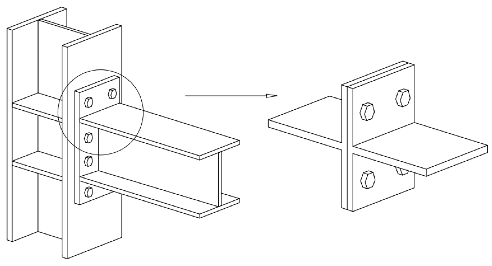
Following the component method provided in Eurocode 3 (EC3) [1], multiple components can be assembled to model steel structural beam-to-column bolted joints [2]. The accuracy of the connection model depends on the accuracy of the stiffness, resistance and ductility of the individual components. One of the components is the T-stub model, which is located in the tension zone of the joint as bolted T-shaped sections (Figure 1). It is used to evaluate the behavior of tensile components that may provide joint ductility due to their high deformation capacity (such as the column flange in bending, the endplate in bending and the bolts in tension). The mechanical behavior of a T-stub is complex because it contains multiple parts that undergo various deformations. Therefore, it is essential to understand the force–displacement curves of axially loaded bolted T-stubs to analyze the moment–rotation responses of semi-rigid bolted joints [3], mainly when using the component method.

Apart from experimental testing, two modelling options are practical for estimating the axially loaded bolted T-stub response: finite element and analytical models.

A finite element model can be used to calculate force–displacement curves for bolted T-stubs. The most accurate results are usually obtained using a three-dimensional finite element method (FEM) model because mechanical and geometric nonlinearities, contact and slip phenomena, residual stresses and bolt preload effects are taken into account. Reinosa [4] developed an advanced 3D finite element (FE) model of a representative T-stub to characterize its deformation response and boundary characteristics related to preloading. The strength and initial stiffness of bolted connections were validated by Wang [5] with T-stub FE models. An FE model of T-stubs subjected to quasi-static tension was developed by Faralli [6]. Deformation maps were shown to reveal the plastic deformation and ultimate failure of T-stubs having a single bolt row. Anwar [7] conducted a parametric study by using a 3D FE model to determine ultimate strength and deformation capacity based on bolt distances and endplate thicknesses. Saleem [8] employed a 3D FE model of notched steel specimens to identify wrinkles leading to the formation of cracks and the deformation capacity, providing a reference for 3D modelling of T-shaped parts.

Solid elements are typically used in the above models, which results in more nodes and larger calculation scales. Using complex 3D finite element models in practical design is still not feasible, and parametric analysis with such models is time-consuming. Therefore, some 2D FE models are proposed. It is expected that 2D FE models will reduce computational scale while ensuring accuracy.

Shell elements were used by Gebbeken [9] to simulate the T-stub’s cross-section, where the thickness of the shell elements corresponds to the bolt diameter and T-stub width. Coelho [10] proposed a 2D FE model based on the prying model of EC3. Francavilla et. al. [11] described a simplified 2D FE model for describing T-stub behavior, which is run on the SAP2000 computer program and can estimate the plastic deformation capacity of bolted joints’ components. FE models in 2D are more efficient than 3D models. As the bolt nut interacts with the T-stub flange, effective width is commonly used to calculate the effect, but this obvious simplification reduces the calculations’ accuracy. As Bursi [12] and Virdi [13] reported, a lack of consideration of 3D behavior may increase the stiffness of 2D models. In addition, most two-dimensional finite element models rely on empirical algorithms based on EC3 to calculate and determine their parameters, making them less accurate. Reinosa [14] combined the analytical component method and the numerical finite element method (FEM) to predict the T-stub’s initial stiffness and deformation capacity. T-stub plates were modelled using four-node quadrangle shell elements, and rotations perpendicular to the elements were included in a complete 3D formulation.

Typically, analytical models use simple mathematical expressions for calculating the response, which offers ease of use but reduces reliability. Analytical models for predicting initial stiffness and plastic resistance have been developed, resulting in design specifications. In this case, EC3 [1] provides design rules for calculating initial stiffness and plastic resistance based on elastic [15,16] and pure plastic theories [17]. However, the approach in EC3 neglects the influence of strain-hardening and nonlinear geometric effects. Subsequently, some theoretical approaches have been proposed to improve the analytical models in EC3. Initially, Piluso [18] attempted to analytically predict the plastic deformation capacity of bolted T-stubs. Mofid [19] decomposed the T-stub assembly into two plates with different or the same boundary conditions and obtained the stiffness of the two plates by the plate and shell mechanics method, respectively. The initial stiffness of the T-stub assembly is obtained after the two plates are superimposed. In this method, the flange deformation in the width direction is considered, but determining the boundary conditions of plates is difficult. According to Loureiro [20], an equivalent model was designed for hand calculations to predict the axial stiffness of the T-stub. T-stub response is calculated analytically based on the flanges and bolts of a beam assembly. Yuan [21] proposed new methods for determining the initial stiffness and plastic resistance of stainless-steel T-stubs, substituting the material yield strength with 3.0% proof strength in the revised formulae. This method is still proposed within the framework of design methods in EC3 and is an extension of the Demonceau model [22]. Piluso [23] and Francavilla [24] developed analytical models of T-stubs based on the assumption of beam yield line mode. Because geometric nonlinearity was not considered in the models, displacements of T-stubs with large deformations are often underestimated. The connection of T-stubs was studied by matrix structural analysis assuming linear and elastic materials and small displacements developed by Reinosa [4]. Francavilla [11] simplified the EC3 model by simplifying the connection between the screw and the lower bolt as directional support, the flange plate as directional support at the web, and the contact between the flange plate and the bottom plate as multiple spring connections. The calculation method for the bearing capacity of the T-stub is obtained. By simplifying the bolt into a spring and the flange plate into a rod with simple support at both ends, Aniello [25] proposed a simplified T-stub model and provided a formula for calculating bearing capacity. This model is an equivalent continuous beam model [15,26], which considers the deformation co-ordination of bolts and flanges, and avoids assuming unreasonable boundary conditions for plates and flanges. However, it is only possible to estimate the initial tensile stiffness and ultimate bearing capacity of T-stubs, not the nonlinear force–displacement relationship during tension.

Scholars have studied the mechanical performance of T-stub components under factors such as prying force and bolt bending moment in recent years. Hantouche [27] simulated the relationship between bolt internal force and external load under different contact forms by placing wedges and flat pads between T-shaped parts and the bottom plate, and proposed a method for calculating the prying force-to-bolt internal force ratio. Subsequently, Hantouche [28] improved the model by assuming that the outer flange plate was articulated to support the bottom plate, that the bolts were simplified as springs, and that the inner flange plate was connected to the web by a fixed-end support with a torsion spring. The displacement balance equation for the model was proposed. Yang [29] developed an improved model to estimate the initial axial tensile stiffness and the ultimate tensile load of T-stubs, including the influence of prying action. Anwar [7] studied the influence of bolt spacing and end plate thickness on the ultimate bearing capacity and deformation capacity of T-stubs. Bao [30] focused on the influence of the bolt bending moment and did not need to calculate the prying force. Instead, he proposed a new model and calculation method for T-stubs using the bending moment stiffness distribution method.

The above models can describe the nonlinear tensioning of T-stubs; however, some limitations apply. First, some models require improvement in terms of accuracy. Taking the model proposed by EC3 as an example, the model overestimates the initial tensile stiffness of T-stubs, and it has errors in describing the force–displacement relationship when T-stubs undergo nonlinear deformation. Second, analysis models provide methods for calculating the initial tensile stiffness and ultimate bearing capacity of T-stubs. However, they cannot describe the force–displacement relationship of the T-stubs in the whole deformation process. Third, the finite element model can describe the nonlinear mechanical behavior of T-stubs, but it is usually based on the traditional contact algorithm. The calculation scale is large, and the calculation efficiency is low. Therefore, it is necessary to propose a new mechanical model of T-stubs to describe the nonlinear force–displacement relationship.

The objective of this study is to develop an accurate representation of the nonlinear tensile behavior of T-stubs using a constitutive model. The tensile tests of T-stubs are carried out in Section 2. The failure modes of T-stubs are summarized, and the force–displacement characteristic curves are derived. In addition, a direct numerical simulation of T-stubs was also performed to obtain the stress distribution characteristics during the tension process and to identify the critical stress states at each of the three stages of the force–displacement curve. Section 3 presents a constitutive model based on the segmented nonlinear characteristics of the force–displacement relationship. Analytical expressions for the proposed model and the identification method for the model parameters were described. Section 4 provides the force–displacement curves characterized by the proposed model and compares them with experimental and EC3 curves.

2. The Behavior of the T-Stub under an Axial Tensile Load

2.1. Experiments

2.1.1. Material Characterization

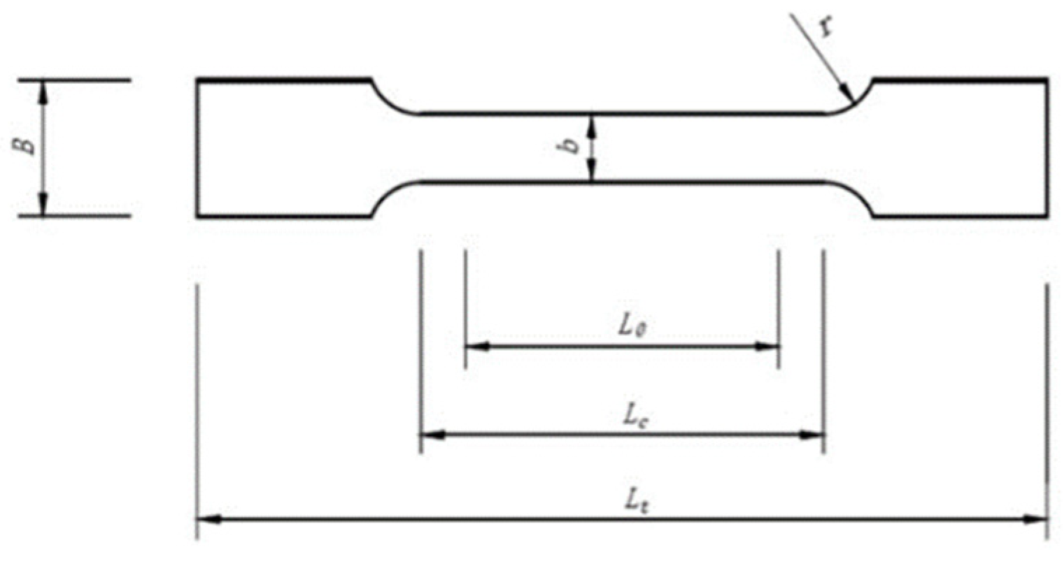
Uniaxial tensile tests were conducted to characterize the mechanical properties of 8 mm and 12 mm Q355 steel. The specimen size was determined by considering the clamping end of the test equipment and the extension gauge distance following the relevant provisions of the national standard GB/T2281-2010 [31]. The section size of the specimen is shown in Figure 2 and

Table 1. Specimen geometry size.

Specimen	$\mathit{t}\mathbf{/}\mathbf{\left(}\mathbf{mm}\mathbf{\right)}$	${\mathit{L}}_0\mathbf{/}\mathbf{\left(}\mathbf{mm}\mathbf{\right)}$	${\mathit{L}}_{\mathit{C}}\mathbf{/}\mathbf{\left(}\mathbf{mm}\mathbf{\right)}$	${\mathit{L}}_{\mathit{t}}\mathbf{/}\mathbf{\left(}\mathbf{mm}\mathbf{\right)}$	$\mathit{B}\mathbf{/}\mathbf{\left(}\mathbf{mm}\mathbf{\right)}$	$\mathit{b}\mathbf{/}\mathbf{\left(}\mathbf{mm}\mathbf{\right)}$	$\mathit{r}\mathbf{/}\mathbf{\left(}\mathbf{mm}\mathbf{\right)}$
C-8-1	8	80	102	238	50	15	18
C-8-2	8	80	102	238	50	15	18
C-8-3	8	80	102	238	50	15	18
C-12-1	12	98	124	256	50	15	18
C-12-2	12	98	124	256	50	15	18
C-12-3	12	98	124	256	50	15	18

Notes: $t$—Thickness of specimen, $L_0$—Original scale of specimen, $L_C$—Length of parallel section of the specimen, $L_t$—Length of specimen, $B$—Width of clamping end of specimen, $b$—Width of parallel section of specimen, $r$—Radius of transition arc.

.

The mechanical property parameters of the material are listed in

Table 2. Tensile test results of Q355 steel.

Specimen	Thickness	Yield Strength ${\mathit{f}}_{\mathit{y}} \left(\mathbf{MPa}\right)$	Yield Strain ${\mathit{\epsilon }}_{\mathit{y}}$	Modulus of Elas-ticity  $\mathit{E} \left(\mathbf{MPa}\right)$	Ultimate Strength ${\mathit{f}}_{\mathit{u}} \left(\mathbf{MPa}\right)$	Ultimate Strain ${\mathit{\epsilon }}_{\mathit{u}}$
C8-1	8	444.2	0.00197	189,789	592.6	0.142
C8-2	8	432.5	0.00194	190,243	586.4	0.134
C8-3	8	439.7	0.00199	191,877	589.3	0.156
C12-1	12	427.1	0.00177	201,898	559.5	0.095
C12-2	12	425.6	0.00179	203,270	556.4	0.076
C12-3	12	415.5	0.00179	202,425	557.1	0.083
average value	-	431.6	0.00188	196,583	595.5	0.11

. A scatter in necking strain was observed as a result of statistical variation in the mechanical properties of the materials tested. The average value of each parameter can be used as the parameter value in subsequent numerical simulations.

2.1.2. Geometric Characteristics of the Specimen

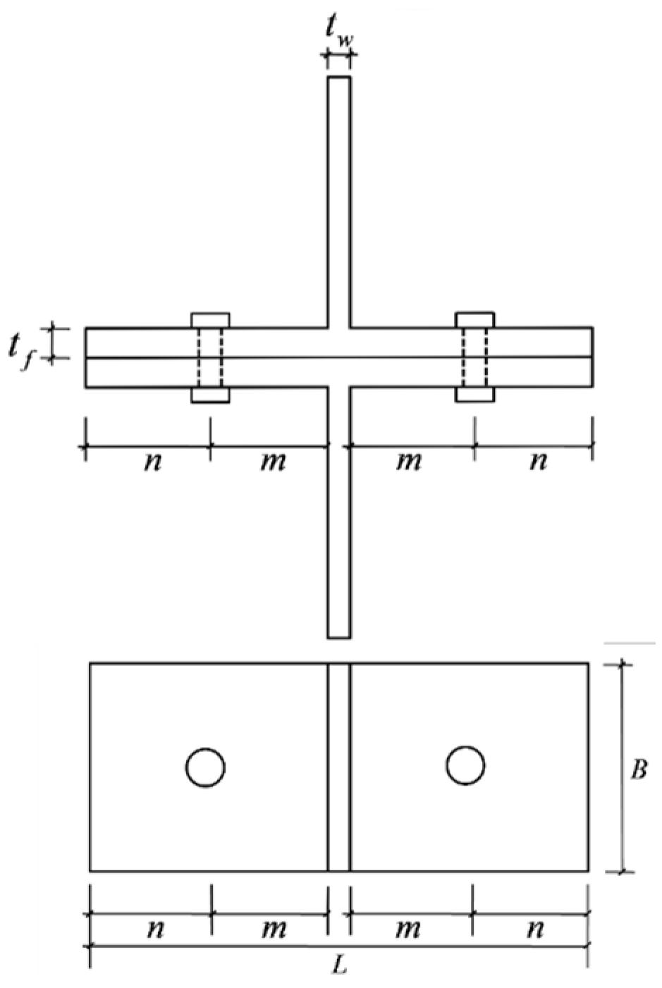
The tested T-stubs were made of two welded plates, the flange and the web, which were joined together by a continuous fillet weld, as shown in Figure 3. Two grade 10.9 bolts connect the flanges of the T-pieces. The geometric parameters of the specimens were designed considering the influence of three factors: flange plate thickness, bolt diameter, and the distance from screw hole to edge. Among them, the end plate thickness and bolt diameter sizes were selected from the typical sizes in engineering. The distance from the screw hole to edge $n$ should comply with the engineering construction requirements in the specification JGJ82-2011 [32]. The margin coefficient $s$ should meet the construction requirements of EC3 [1], which is $s\le 1.25$. The geometric parameters of the specimen are shown in Figure 3 and

Table 3. Size and preload force of T-stub.

Specimen	${\mathit{t}}_{\mathit{f}} \left(\mathbf{mm}\right)$	${\mathit{t}}_{\mathit{w}} \left(\mathbf{mm}\right)$	$\mathit{n} \left(\mathbf{mm}\right)$	$\mathit{m} \left(\mathbf{mm}\right)$	$\mathit{s}$	$\mathit{L} \left(\mathbf{mm}\right)$	$\mathit{B} \left(\mathbf{mm}\right)$	$\mathit{d} \left(\mathbf{mm}\right)$	$\mathit{P} \left(\mathbf{kN}\right)$
D14	14	12	60	100	0.6	332	80	18	110
D16	16	12	60	100	0.6	332	80	18	110
D18	18	12	60	100	0.6	332	80	18	110
S90	16	12	70	90	0.78	332	80	18	110
S80	16	12	80	80	1.0	332	80	18	110
M20	16	12	60	100	0.6	332	80	22	150
M24	16	12	60	100	0.6	332	80	26	225

Notes: $P$—Bolt preload, $s=n/m$.

. In addition, the bolt preload value is determined according to the design value in the specification [32], as listed in Table 3.

It is polished so that the horizontal plane of the flange plate is perpendicular to the facade web. Before applying the preload, ensure the upper and lower T-shaped parts are in close contact without any gaps. The specimen is shown in Figure 4.

2.1.3. Test Procedure and Instrumentation

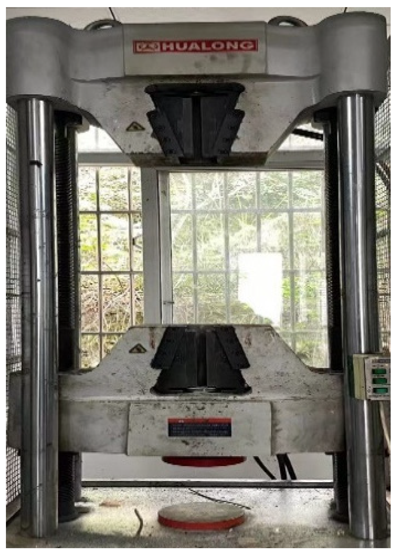
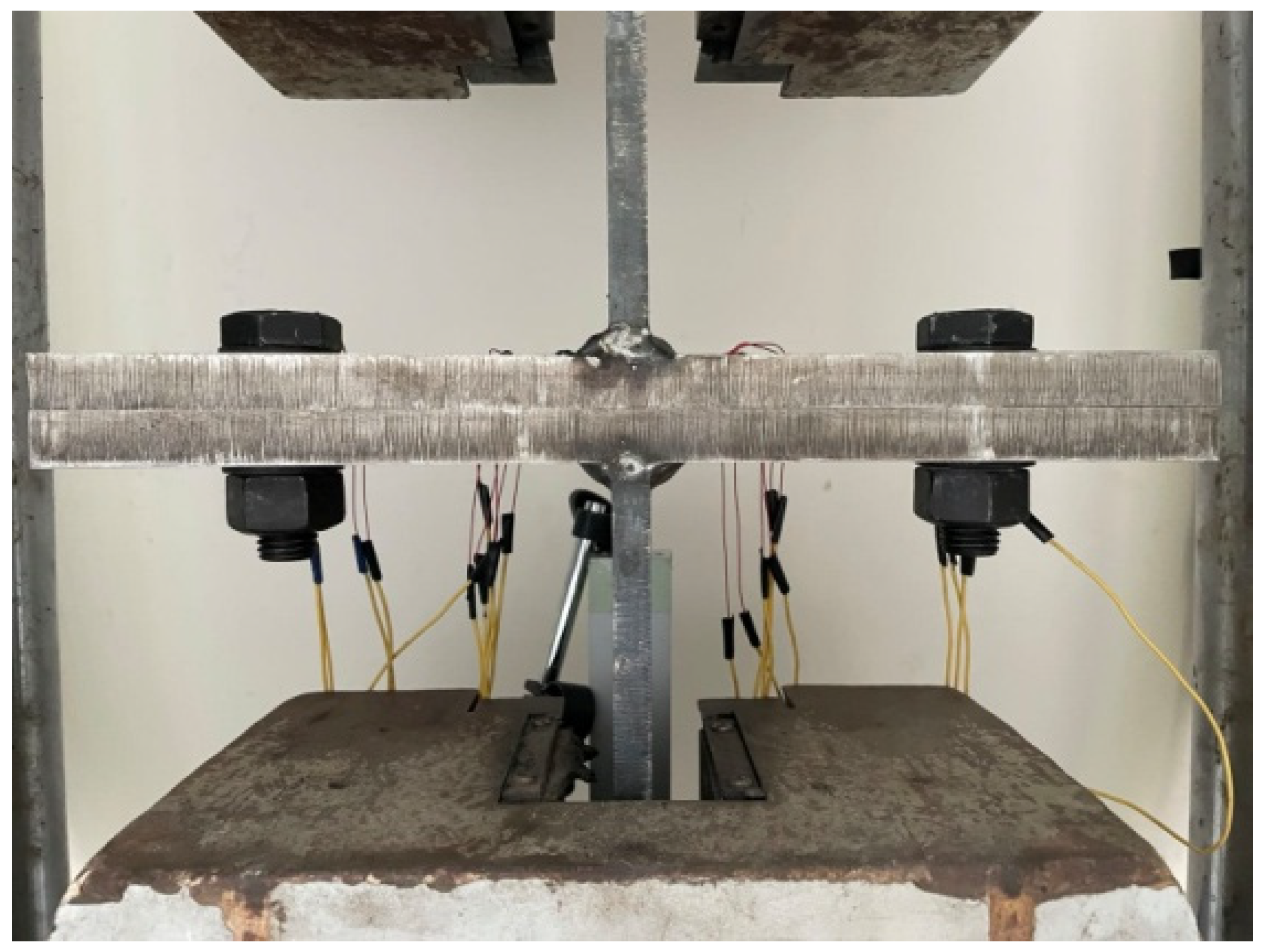
A Hualong universal testing machine was used to test bolted T-stubs under displacement control at 0.05 mm/s (see Figure 5 load capacity +/600 kN, stroke 300 mm), where a machine load cell and displacement transducer were used to measure overall deformation. Figure 6 shows that an axial load was applied to the clamped web.

2.1.4. Experimental Results

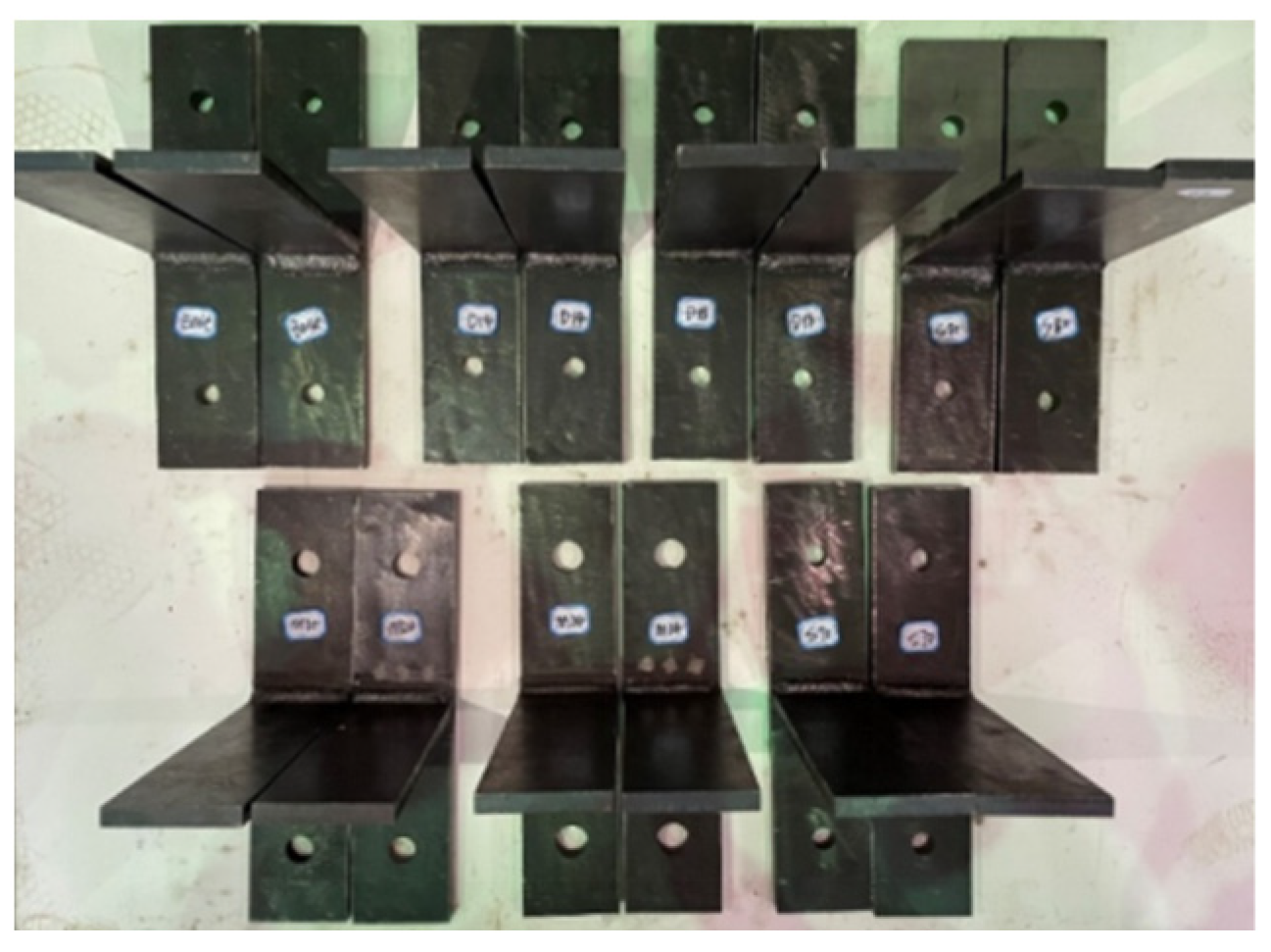
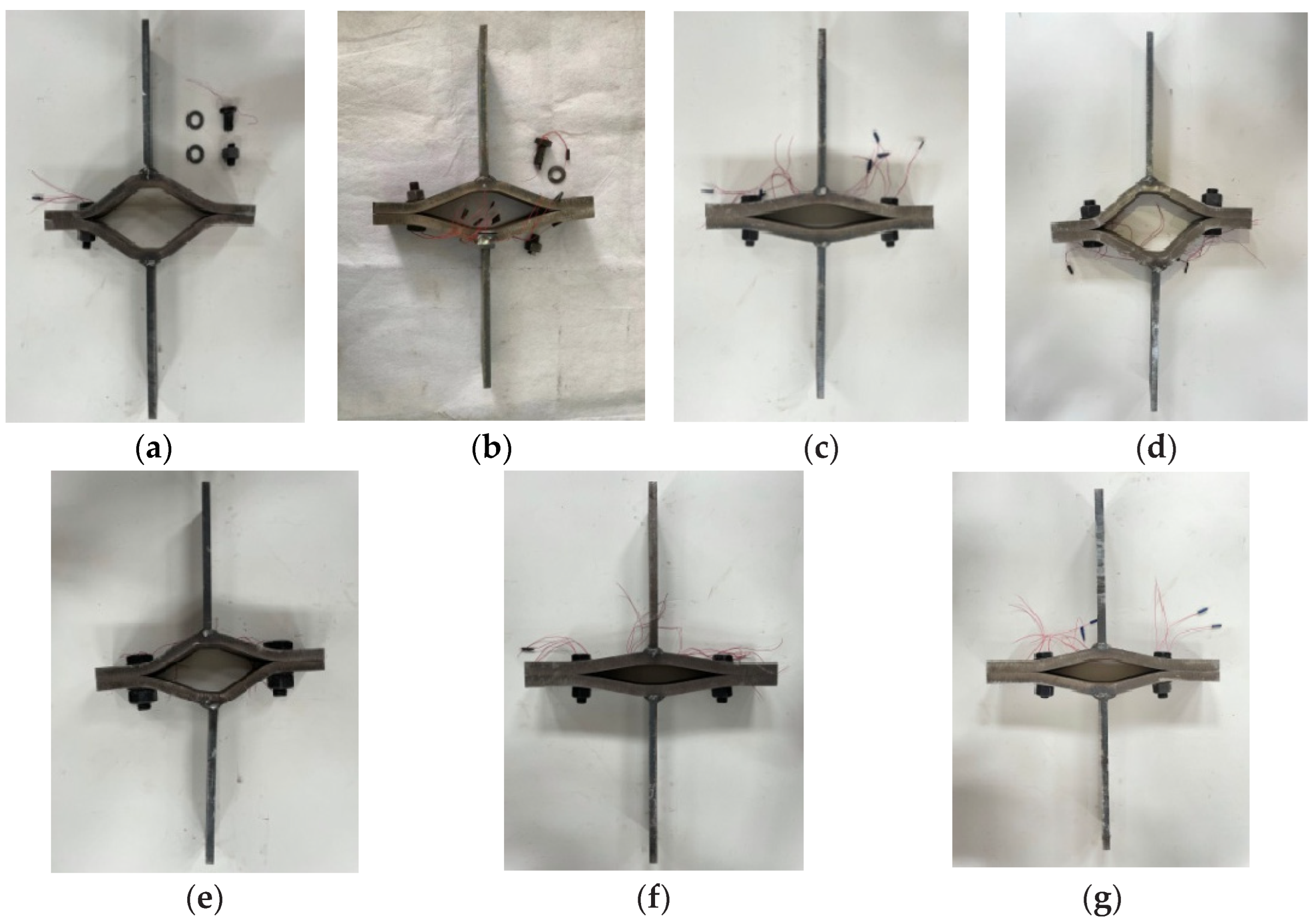
The selected T-stubs will either develop a Type-1 failure mechanism (plate yield) or a Type-2 failure mechanism (plate yield in combination with bolt failure in tension), as described in EC3 Part 1.8 [1]. Figure 7 shows the post-test T-stub specimens which all failed in either a Type-1 or Type-2 manner.

Figure 7. Post-test (failed) specimens—see Table 4 for the classification of their failure mode. (a) D14, (b) D16, (c) D18, (d) M20, (e) M24, (f) S70, (g) S80.

Figure 7. Post-test (failed) specimens—see Table 4 for the classification of their failure mode. (a) D14, (b) D16, (c) D18, (d) M20, (e) M24, (f) S70, (g) S80.

Taking M20 as an example, Type-1 damage occurs. The flange plates of T-shaped pieces were in close contact at the beginning of loading. Due to the increased load, there was a gap between the flange plates, and bending deformation occurred to the bolt rod. A plastic hinge or seam toe crack appears when the connection between the flange plate and the web fails. In specimen D16, a Type-2 failure occurred. The upper and lower flange plates of the T-shaped piece are in close contact during initial loading. When the load increases, the flange plates bend, and the gap widens rapidly. Plastic hinge or weld toe cracks appear between the flange plate and web at the time of failure, and the bolt is broken.

Table 4. Failure modes for test specimens.

Plate yielding (Type-1)	D18 M20 M24 S70 S80
Plate yielding together with bolt failure (Type-2)	D14 D16

Table 4. Failure modes for test specimens.

Plate yielding (Type-1)	D18 M20 M24 S70 S80
Plate yielding together with bolt failure (Type-2)	D14 D16

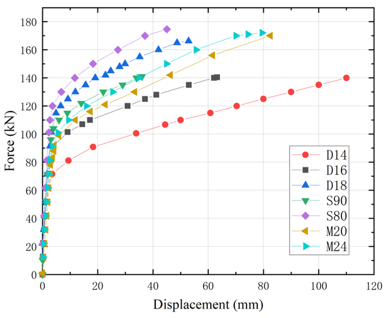
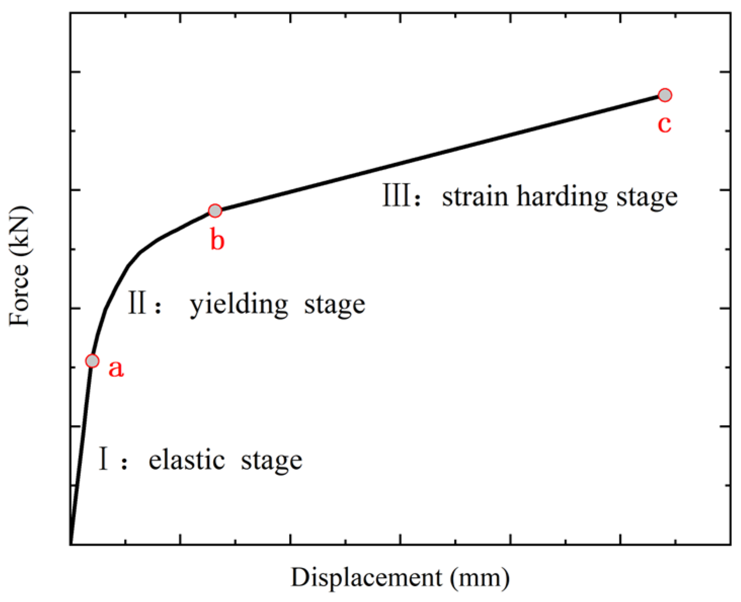
The force–displacement curves and mechanical properties of T-stubs can be obtained, as shown in Figure 8 and

Table 5. Mechanical properties parameters of test T-type specimens.

Specimen	Yield Load (kN)	Yield Displacement (mm)	Ultimate Load (kN)	Ultimate Displacement (mm)	Initial Tensile Stiffness (kPa)
D14	71	2.1	140	110	30,809
D16	91	3.9	141	62	32,105
D18	110	3.2	166	52	34,375
S90	98	2.9	141	36	33,793
S80	102	2.3	174	45	44,347
M20	92	4.2	170	83	21,749
M24	101	5.6	172	79	18,035

. Based on the experimental phenomena and the force–displacement curves, it can be demonstrated that the load–displacement curves of the T-stub are segmented nonlinear. Depending on the geometry of the T-stub, the slope of its force–displacement curve varies. Their processes, however, are similar. It is shown in Figure 8 that the first stage in the process is elastic deformation, where the force–displacement curve is linear. There was no obvious deformation in the flange plates, which were in close contact with one another. A gap appears between the flange plates as the load increases. At this point, the T-stubs enter stage two: the yield stage, where the force–displacement curve becomes nonlinear. During this stage, the flange plate gap slowly increases, and then evident bending occurs until the local area of the specimen yields. With increasing loads, the yielding area of the T-stub expands, resulting in the gap between upper and lower T-shaped flange plates increasing rapidly. The third stage is the strain-hardening stage. After yielding, the T-stubs still retain residual stiffness, and the force–displacement curve is almost linear until they reach tensile capacity, which is represented by point c in Figure 9.

2.2. Three-Dimensional Nonlinear Finite Element Analysis

2.2.1. Finite Element Model

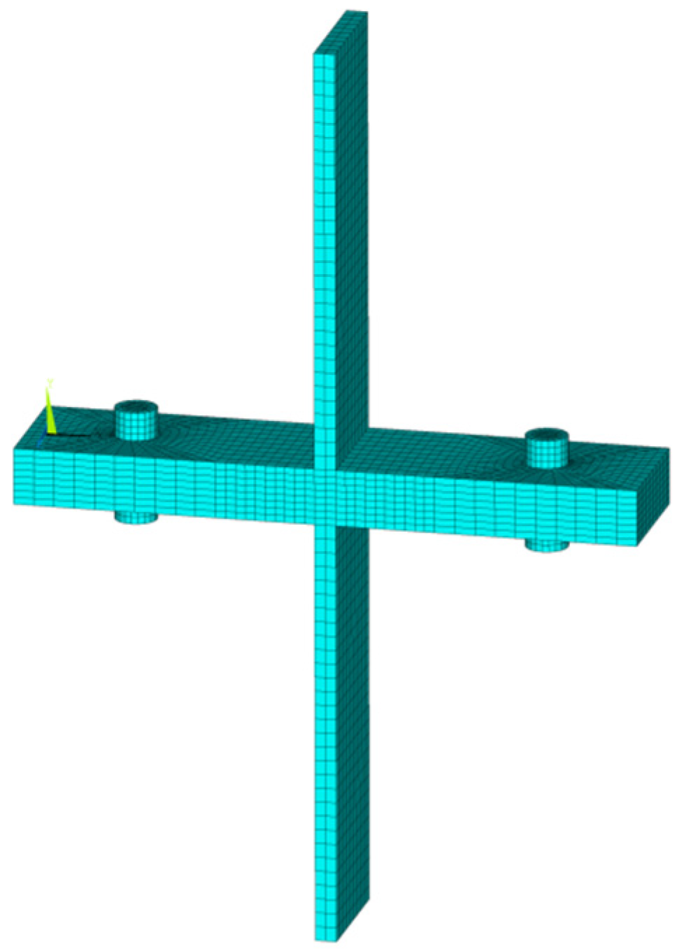
Finite element simulations of T-stub specimens were conducted using ANSYS software to clarify stress distribution characteristics throughout the loading process (Figure 10). Based on the test results, it was assumed that the specimen would not fracture at the welds, so the flange and web of the T-stubs were modelled directly as a whole in the numerical model.

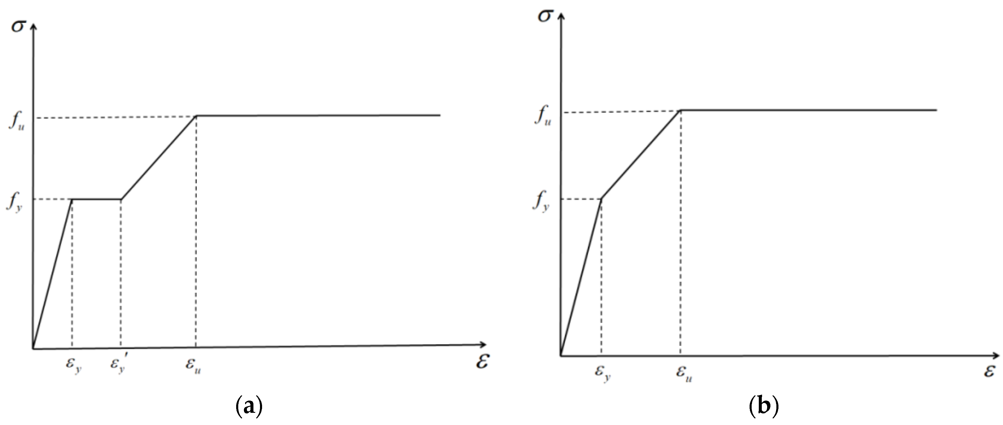
The SOLID45 elements were used to simulate the T-stubs. In this study, the materials were considered to be isotropic and assumed to be an ideal four- or three-linear elastoplastic model. Figure 11a illustrates the stress–strain relationship of Q355 steel as a four-line follow-up strengthening model, whereas Figure 11b illustrates the stress–strain relationship of 10.9 high-strength bolt as a three-line follow-up strengthening model. The value of material parameters of Q355 steel is based on the tensile test results of Q355 steel in Section 2.1, as shown in

Table 6. Mechanical property parameters of steel material Q355.

Yield Strength ${\mathit{f}}_{\mathit{y}} \left(\mathbf{M}\mathbf{P}\mathbf{a}\right)$	Yield Strain ${\mathit{\epsilon }}_{\mathit{y}}$	Elasticity Modulus E $\left(\mathbf{M}\mathbf{P}\mathbf{a}\right)$	Strain ${\mathit{\epsilon }}_{\mathit{y}}^{\prime }$	Ultimate Strength ${\mathit{f}}_{\mathit{u}} \left(\mathbf{M}\mathbf{P}\mathbf{a}\right)$	Ultimate Strain ${\mathit{\epsilon }}_{\mathit{u}}$
431.6	0.00188	196,583	0.015	595.5	0.11

. According to the product quality guarantee, the material parameters for 10.9 s high-strength bolt were set as shown in

Table 7. Mechanical properties of high-strength bolt 10.9 s.

Yield Strength ${\mathit{f}}_{\mathit{y}} \left(\mathbf{M}\mathbf{P}\mathbf{a}\right)$	Yield Strain ${\mathit{\epsilon }}_{\mathit{y}}$	Elasticity Modulus $\mathit{E} \left(\mathbf{M}\mathbf{P}\mathbf{a}\right)$	Ultimate Strength ${\mathit{f}}_{\mathit{u}} \left(\mathbf{M}\mathbf{P}\mathbf{a}\right)$	Ultimate Strain ${\mathit{\epsilon }}_{\mathit{u}}$
995	0.00483	206,004	1160	0.136

. Furthermore, Poisson’s ratio was 0.3, and the von Mises yield criterion was applied.

There are contact pairs between the nuts and the flange plates and between the upper and lower flanges. CONTA174 and TARGE170 elements were used for the contact and target elements, respectively. A contact surface can be separated along its normal direction and can slide relative to another along its tangent direction. In addition, the friction coefficient of the contact surface was set at 0.44. A pretightening force was applied through PRETS179, and the preload value was the same as in the test, as shown in Table 3.

The lower T-stub web was set as a fixed constraint, while the upper T-stub web applied a displacement load. The displacement load value refers to the ultimate displacement obtained by the test, as listed in Table 3. Two load steps were applied to the T-stubs. In the first step, preload was applied to the bolt, and slight deformation static analysis was used; in the second step, displacement load was applied to the T-stub web, and large deformation static analysis was used.

2.2.2. Analysis of Finite Element Model Results

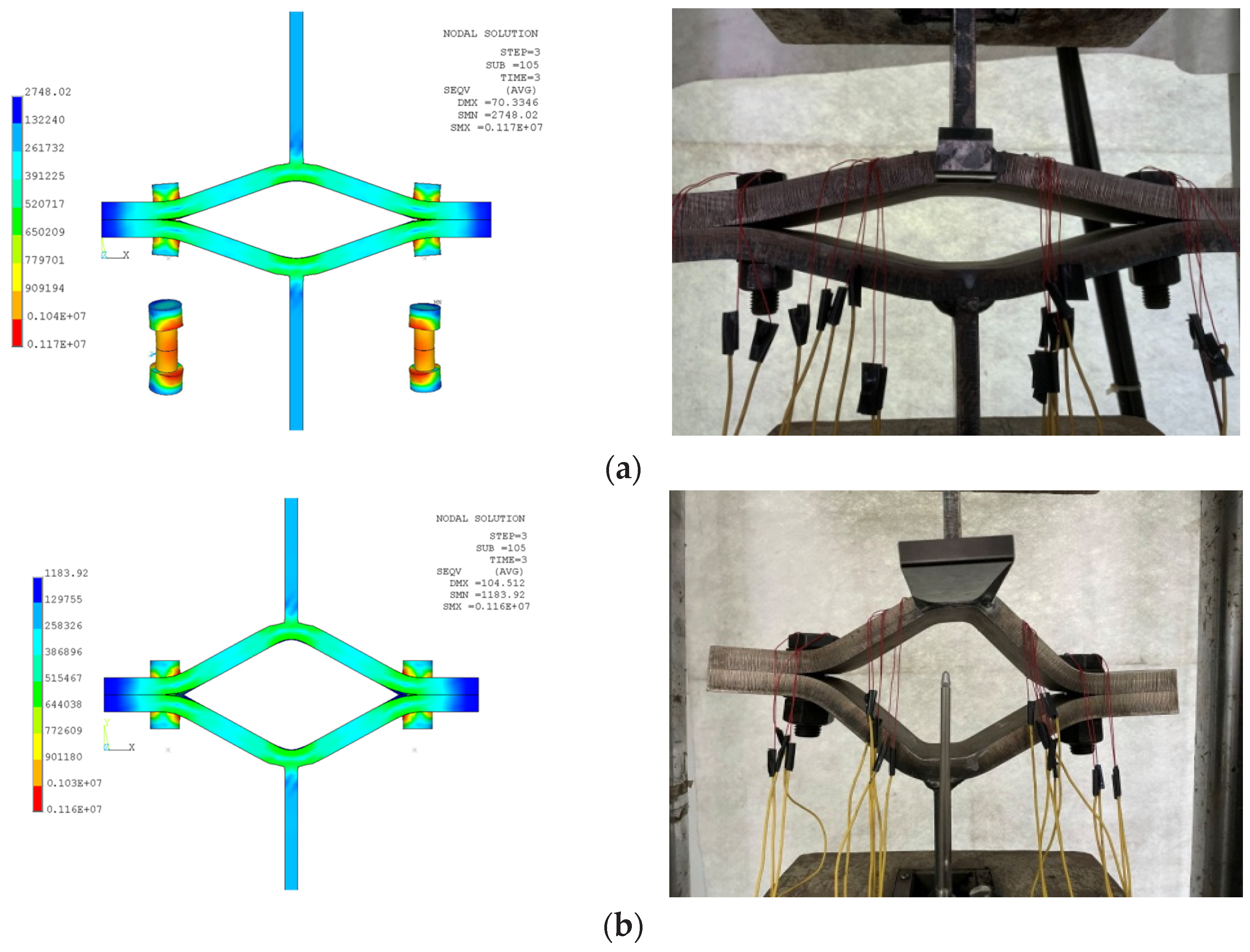
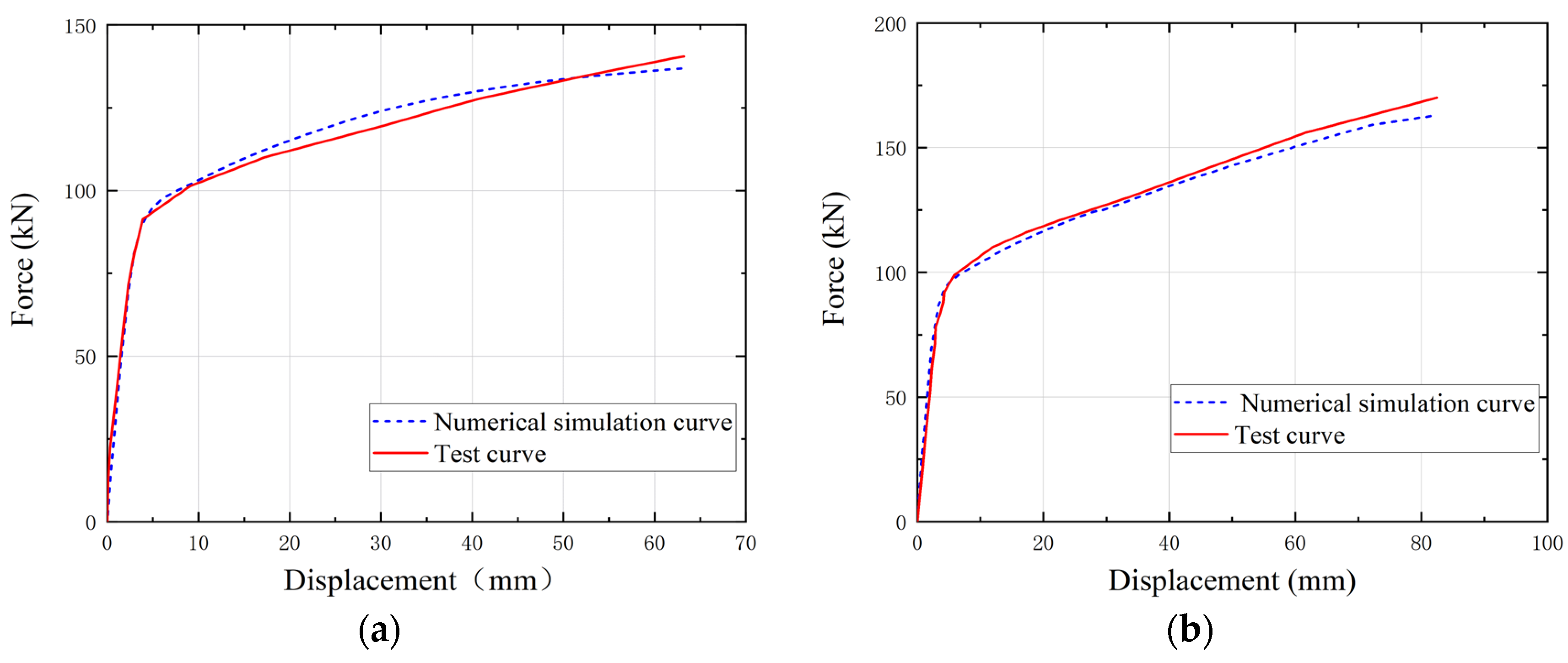
Taking specimens D16 and M20 as examples to illustrate the simulation results, a comparison of the simulated T-stub deformation with the experimental phenomenon is shown in Figure 12. The simulation results indicate that the flange plate of the D16 and M20 specimens exhibits significant bending deformation, and the plastic hinge appears at the connection part between the web and the flange plate. Additionally, the bolts in the D16 specimen showed obvious bending deformation, reaching ultimate strength in some areas, and the bolts failed. Simulated specimens deform essentially the same way as test specimens in the limit state. The force–displacement curves of T-stubs obtained by numerical simulation also agree with those obtained by experiment, as shown in Figure 13.

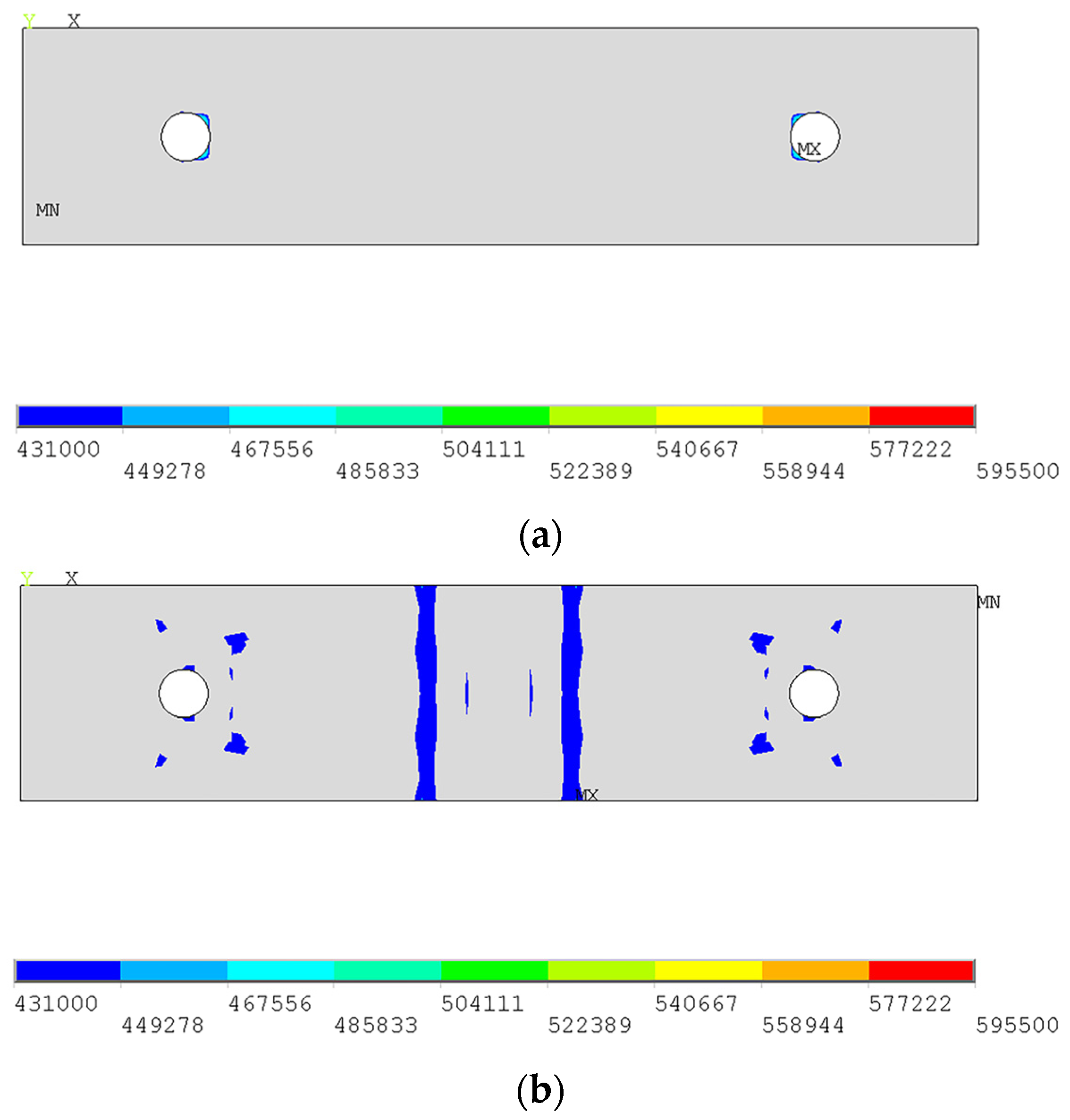
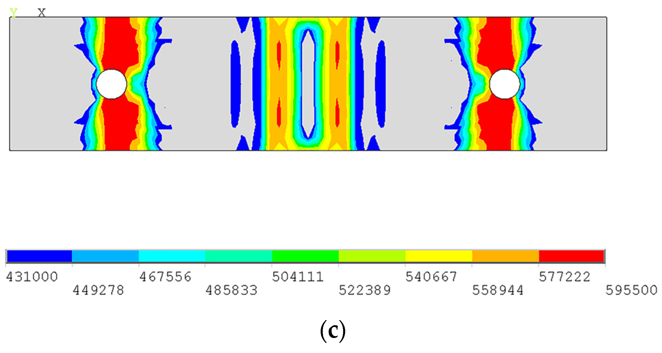
Based on the numerical simulation results, it is evident that the stress distribution of T-stubs exhibits three key states. In the first state, the area around the screw hole yields, as shown in Figure 14a. With increasing load, the second state occurs: the joint between the flange plate and web yields, and the yield area is connected along the width of the flange plate, as shown in Figure 14b. The third state is the limit state. Flange plates have obvious plastic deformations. The material at the connection part between the flange plate and web and the area around the bolt hole has yielded and reached the ultimate tensile strength, as shown in Figure 14c. The critical states of the above three stress distributions correspond to points a, b, and c on the force–displacement curve shown in Figure 9.

3. Mechanical Model of T-Stubs

3.1. The Constitutive Relation

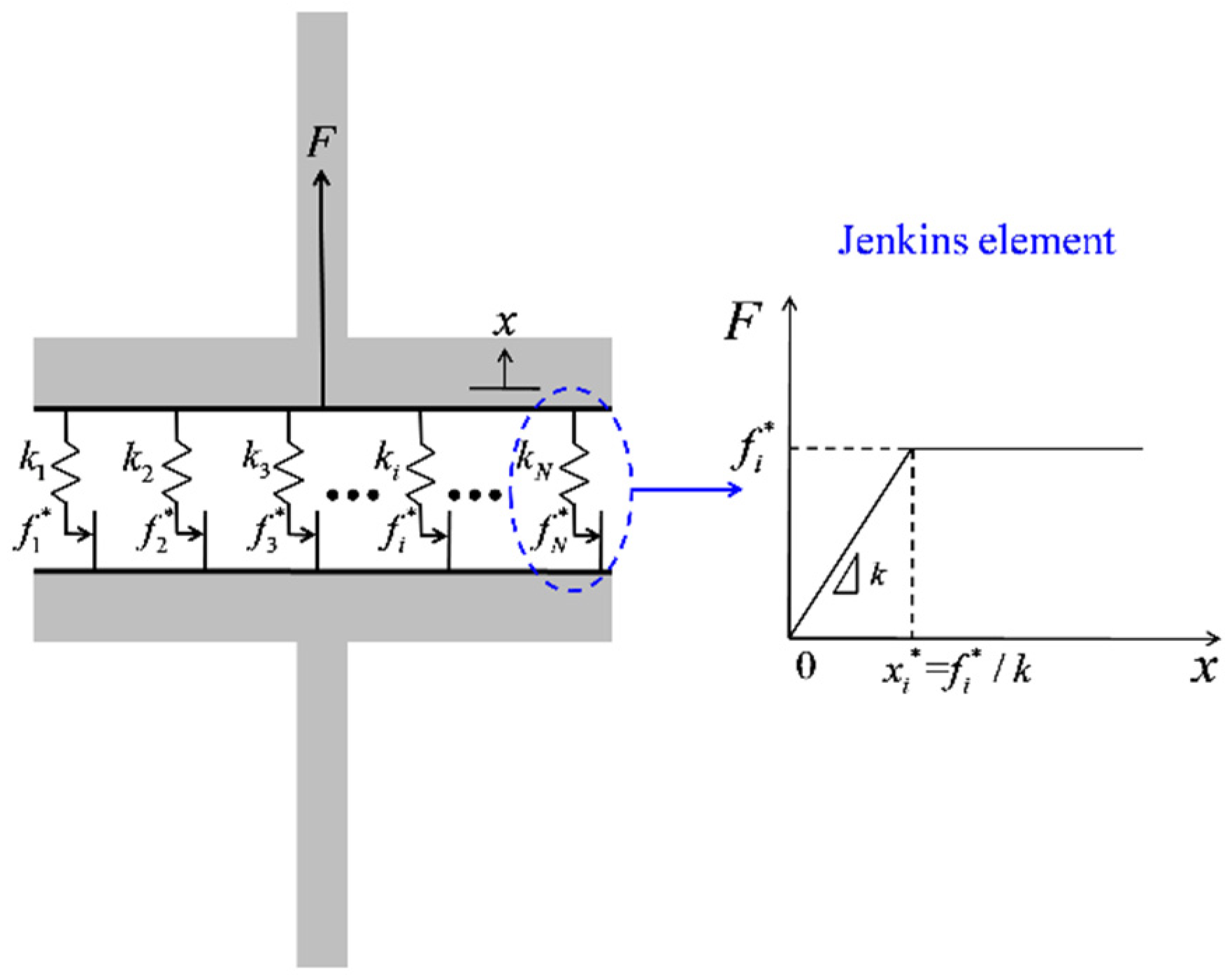
Based on the behavior characteristics of T-stubs under tension, the Iwan model [33] is adopted to establish the mechanical model of T-stubs. The model is composed of a series of Jenkins elements connected in parallel, and each Jenkins element is formed of a spring and a slider in succession, as shown in Figure 15. The force of each Jenkins element can be expressed as follows [33]:

$$f_i=f_i(x)=\left\{\begin{array}{l}{k}_{i}x 0<x\le x_i^{*}\\ k_i{x}_i^{*} x>x_i^{*}\end{array}\right.$$

(1)

In the model, $k_i$ represents the stiffness of the spring, $x$ represents the displacement, the Jenkins element’s yielding displacement is described by $x_i^{*}$, and the Jenkins element’s yielding force, $k_i{x}_i^{*}$, is represented by the symbol $f_i^{*}$.

A parallel–series model is formed by connecting Jenkins elements in parallel. A natural connection can be viewed as an idealized connection, where the Iwan model is applied to the contact interfaces between upper and lower T-stubs, as shown in Figure 15. It is worth noting that the Iwan model here represents the force–displacement relationship of the T-stubs under tension rather than the conventional representation of the tangential slip of the interface.

The force–displacement relationship of the model can be expressed as follows [33]:

$$F=F(x)={\displaystyle \sum _{i=1}^n{f}_i+}{\displaystyle \sum _{j=n+1}^N{k}_{j}x}$$

(2)

where $N$ is the total number of Jenkins elements, $x$ is the monotonically increasing displacement, $n$ represents the number of yielding elements. Thus, the first and second parts of Equation (2) represent the summation of the forces on the yielded and remain elastic Jenkins elements, respectively.

When $\mathrm{N}\to \infty$, the distribution function $\phi \left(f\right)$ can be used to express the yielding force $f_i^{*}$ of the Jenkins element. Assuming that $k_i$ is identical and expressed as $k$. Then Equation (2) can be rewritten as [34]:

$$F(x)={\displaystyle {\int }_0^{kx}f\cdot \phi (f)\mathrm{d}f+{\displaystyle {\int }_{kx}^{\infty }kx\cdot \phi (f)}}\mathrm{d}f$$

(3)

Equation (3) can be double differentiated to determine the distribution function $\phi f$, as shown below:

$$\phi (f)={\left.-\frac{1}{k^2}\frac{{\partial }^{2}F(x)}{\partial x^2}\right|}_{f=kx}$$

(4)

The unknown parameter $k$ is removed from the Equation (4) by variable substitution:

$$\rho (\lambda )=\frac{f}{k}, \lambda =k^2\phi (f)$$

(5)

As a result, the Iwan model can be expressed as follows:

$$F(x)={\displaystyle {\int }_0^x\lambda \rho (\lambda )}\mathrm{d}\lambda +{\displaystyle {\int }_x^{\infty }x\rho (\lambda )}\mathrm{d}\lambda$$

(6)

Using the nonlinear characteristics of the T-stub’s force–displacement curve, a uniform density function [35] is proposed in this study that assumes the stiffness in the strain-hardening stage of the T-stub’s tension to be linear. In other words, it can be expressed as follows:

$$\rho (\lambda )=\left\{\begin{array}{l}R[H(\lambda -{\lambda }_1)-H(\lambda -{\lambda }_2)]+K_{\infty }\delta (\lambda -{\lambda }_{\infty }),\begin{array}{ccc}& & \lambda >0\end{array}\\ 0,\begin{array}{ccc}& & \lambda =0\end{array}\end{array}\right.$$

(7)

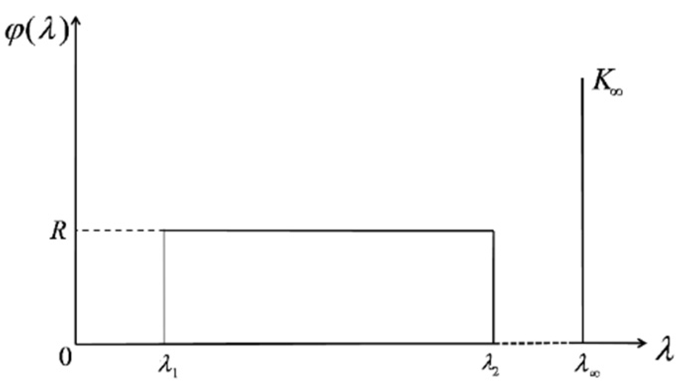
where $H\left(\lambda \right)$ is the Heaviside step function, and $\delta \left(\lambda \right)$ is the Dirac delta function. Using the displacement dimensions, ${\lambda }_1$ and ${\lambda }_2$ represent the initiation positions of yielding and strain-hardening, respectively. The yielding force distribution is described by parameter $R$. $K_{\infty }$ is the residual tensional stiffness after yielding of the T-stub. To ensure a constant $K_{\infty }$ throughout the strain-hardening process, ${\lambda }_{\infty }$ is defined as a point on the $\lambda$-axis sufficiently distant from ${\lambda }_2$, and will not be discussed. Figure 16 illustrates the density function $\phi \left(\lambda \right)$ graphically.

3.2. Backbone Equation

In the Iwan model, the backbone curve represents the force–displacement relationship under monotonic external loads. Substituting Equation (7) into Equation (6) yields the following:

If $0\le \theta <{\lambda }_1$,

$$\begin{array}{ll}F(x)& ={\displaystyle {\int }_{{\lambda }_1}^{{\lambda }_2}xR}\mathrm{d}\lambda +{\displaystyle {\int }_{{\lambda }_2}^{\infty }x{K}_{\infty }\delta (\lambda -{\lambda }_2)}\mathrm{d}\lambda \\ & =\left[R({\lambda }_2-{\lambda }_1)+K_{\infty }\right]x\end{array}$$

(8)

If ${\lambda }_1\le x<{\lambda }_2$,

$$\begin{array}{ll}F(x)& ={\displaystyle {\int }_{{\lambda }_1}^x\lambda R}\mathrm{d}\lambda +{\displaystyle {\int }_x^{{\lambda }_2}xR}\mathrm{d}\lambda +{\displaystyle {\int }_{{\lambda }_2}^{\infty }x{K}_{\infty }\delta (\lambda -{\lambda }_2)}\mathrm{d}\lambda \\ & =(R{\lambda }_2+K_{\infty })x-\frac{R({\lambda }_1^2+x^2)}{2}\end{array}$$

(9)

If $x\ge {\lambda }_2$,

$$\begin{array}{ll}F(x)& ={\displaystyle {\int }_{{\lambda }_1}^{{\lambda }_2}\lambda R}\mathrm{d}\lambda +{\displaystyle {\int }_{{\lambda }_2}^{\infty }x{K}_{\infty }\delta (\lambda -{\lambda }_2)}\mathrm{d}\lambda \\ & =\frac{R({\lambda }_2^2-{\lambda }_1^2)}{2}+K_{\infty }x\end{array}$$

(10)

Equations (8)–(10) can be combined to form the backbone equations of the model:

$$F(x)=\left\{\begin{array}{l}\left[R({\lambda }_2-{\lambda }_1)+K_{\infty }\right]x, 0\le x<{\lambda }_1\\ (R{\lambda }_2+K_{\infty })x-\frac{R({\lambda }_1^2+x^2)}{2}, {\lambda }_1\le x<{\lambda }_2\\ \frac{R({\lambda }_2^2-{\lambda }_1^2)}{2}+K_{\infty }x, x\ge {\lambda }_2\end{array}\right.$$

(11)

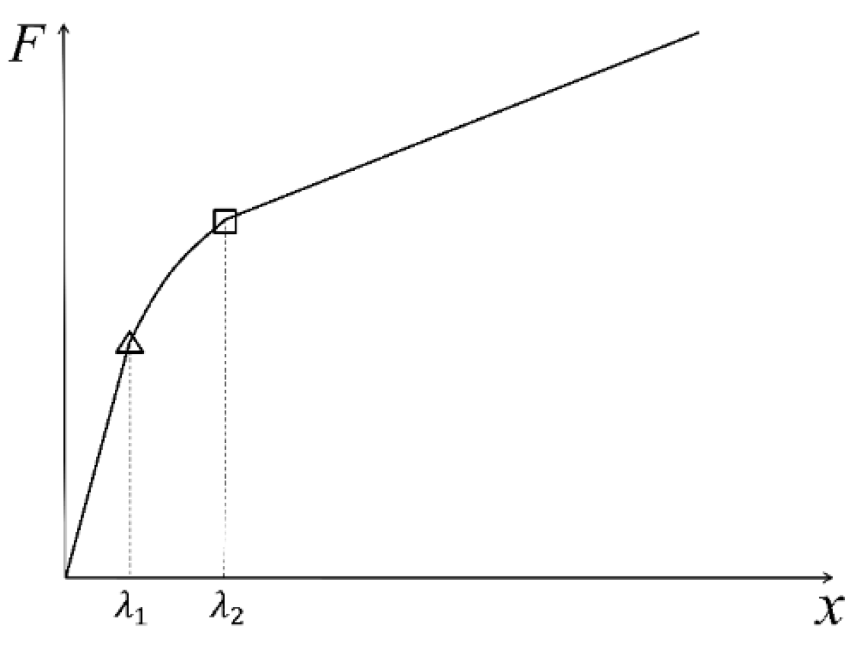
Figure 17 shows the backbone curve according to Equation (11), where the symbols △ and □ denote the initial positions of the yielding and strain-hardening phases, respectively. None of the Jenkins elements yields, the Iwan model shows the behavior of a linear spring before yielding, and the force–displacement graph is linear based on the first part of Equation (11). Several Jenkins elements begin to fail as the curve becomes nonlinear in the second part of Figure 17. In the third part, all the Jenkins elements yield during the strain-hardening stage, leaving only one spring element as a residual stiffness. Therefore, the model behaves as a linear spring when the force–displacement relationship becomes linear again.

The tensional stiffness function can be calculated by differentiating Equation (11) for displacement $x$ as follows:

$$K(x)=\left\{\begin{array}{l}R({\lambda }_2-{\lambda }_1)+K_{\infty }, 0\le x<{\lambda }_1\\ R({\lambda }_2-x)+K_{\infty }, {\lambda }_1\le x<{\lambda }_2\\ K_{\infty }, x\ge {\lambda }_2\end{array}\right.$$

(12)

Equation (12) shows that the model’s tensile stiffness is constant across the elastic range. As the T-stub connection yields, the model’s tensile stiffness decreases linearly. During the strain-hardening stage, the model’s tensile stiffness becomes constant again.

3.3. Parameter Identification of the Model

The constitutive model of T-stubs contains three parameters, which are: the displacement at the beginning of the yielding phase ${\lambda }_1$, the displacement at the beginning of the strain-hardening phase ${\lambda }_2$, and the residual stiffness of the model $K_{\infty }$. ${\lambda }_1$ and ${\lambda }_2$ are identified by referring to the definition in Section 2, which correspond to the displacements of states a and b in Figure 9, respectively.

$K_{\infty }$ is the slope of the strain-hardening section of the force–displacement curve of T-stubs, which can be determined according to the following equation:

$$K_{\infty }=\frac{F_u-F_{{\lambda }_2}}{{\lambda }_u-{\lambda }_2}$$

(13)

where $F_u$ and ${\lambda }_u$ represent the ultimate load and ultimate displacement of T-stubs, respectively. $F_{{\lambda }_2}$ denotes the force corresponding to the initiation position of the strain-hardening stage ${\lambda }_2$ on the force–displacement curve.

In addition, the parameter $R$ describes each Jenkins element’s yielding force distribution. The yielding force $F_{\mathrm{s}}$ of the T-stubs can be obtained using Equation (14):

$$F_s=F({\lambda }_2)=\frac{{\lambda }_2^2-{\lambda }_1^2}{2}R+K_{\infty }{\lambda }_2$$

(14)

Accordingly, Equation (14) can be solved in order to determine the parameter $R$.

4. Model Validation

Table 8. Parameter identification results of the specimens.

Specimen	${\mathit{\lambda }}_1 \left(\mathbf{m}\right)$	${\mathit{\lambda }}_2 \left(\mathbf{m}\right)$	${\mathit{K}}_{\mathit{\infty }} (\mathbf{kN}/\mathbf{m})$	$\mathit{R} \left({\mathbf{kN}/\mathbf{m}}^2\right)$	${\mathit{F}}_{{\mathit{\lambda }}_2} \left(\mathbf{kN}\right)$
D16	0.0015	0.0057	797.7	5,969,109	94.8
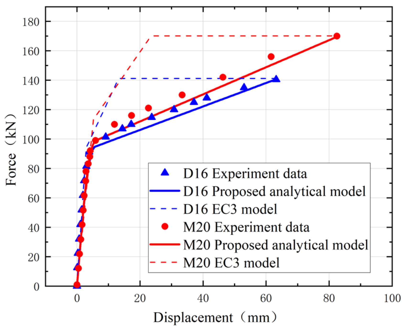
M20	0.0015	0.0059	920.9	5,747,346	99

shows the results of the parameter identification method used on specimens D16 and M20. The comparisons of the force–displacement curves for D16 and M20 T-stubs obtained from the proposed analytical model and EC3 model with the test results are shown in Figure 18.

It can be seen from Figure 18 that the EC3 model curves corresponded closely with the test findings during the elastic deformation stage. However, the slope of the EC3 model curves was significantly larger than the test data when T-stubs entered the nonlinear deformation stage. The slope of the EC3 model curves became zero after yielding, indicating that the EC3 model cannot characterize the residual tensile stiffness of the T-stubs, which is inconsistent with the test result. In the yielding and strain-hardening stages, the EC3 model curves lay above the test curves. In contrast, the proposed analytical model curves agree better with the test curves in the initial elastic, nonlinear yielding and strain-hardening phases compared to the EC3 model curves.

5. Conclusions

In this study, tensile tests of T-stubs with different geometric sizes were carried out. Based on the test data and experimental phenomena, the force–displacement characteristic curves of T-stubs were obtained. The characteristic curves show that the force–displacement curves of T-stubs can be divided into the elastic stage, nonlinear yield stage and linear strain-hardening stage.

In addition, a four-parameter constitutive model based on a uniform distribution has been proposed to describe the nonlinear tension characteristics of T-stubs. Model parameters have a clear physical meaning, and their values can be determined from the experimental and numerical simulation results. It has been found that the model suggested in this study is more applicable than the EC3 model and may be utilized to accurately represent the force–displacement relationship of T-stubs under tension.

It is difficult to obtain the force–displacement relationship of T-stubs when modelling the rotation of semi-rigid joints using the component method. Calculations with traditional FEM or analytical methods are either inefficient or inaccurate. In this study, a model is presented to describe the force–displacement relationship more conveniently. In future research, the T-stub constitutive model can be applied to characterize the rotational behavior and energy dissipation properties of semi-rigid joints.

References

- Eurocode 3: Design of Steel Structures–Part 1–8: Design of Joints; European Committee for Standardization: Brussels, Belgium, 2005.
- Li, X.; Tao, L.; Liu, M. Force Transfer Mechanism and Component-Based Model of Cast-Steel-Stiffened Circular-Tube-Column Frames for Progressive Collapse Analysis. Buildings 2022, 12, 1049. [Google Scholar] [CrossRef]
- Piluso, V.; Faella, C.; Rizzano, G. Structural Semi-Rigid Connections: Theory, Design and Software; CRC Press: Boca Raton, FL, USA, 2000. [Google Scholar]
- Reinosa, J.; Loureiro, A.; Gutierrez, R.; Lopez, M. Analytical frame approach for the axial stiffness prediction of preloaded T-stubs. J. Constr. Steel Res. 2013, 90, 156–163. [Google Scholar] [CrossRef]
- Wang, Z.; Tizani, W.; Wang, Q. Strength and initial stiffness of a blind-bolt connection based on the T-stub model. Eng. Struct. 2010, 32, 2505–2517. [Google Scholar] [CrossRef]
- Faralli, A.; Tan, P.; McShane, G.; Wrobel, P. Deformation maps for bolted T-stubs. J. Struct. Eng. 2020, 146, 04020045. [Google Scholar] [CrossRef]
- Anwar, G.A.; Dinu, F.; Ahmed, M. Numerical study on ultimate deformation and resistance capacity of bolted T-stub connection. Int. J. Steel Struct. 2019, 19, 970–977. [Google Scholar] [CrossRef]
- Saleem, A.; Tamura, H.; Katsuchi, H. Change in Surface Topography of Structural Steel under Cyclic Plastic Deformation. In FFW 2021: Proceedings of the 9th International Conference on Fracture, Fatigue and Wear; Springer: Berlin/Heidelberg, Germany, 2022; pp. 175–193. [Google Scholar]
- Gebbeken, N.; Rothert, H.; Binder, B. On the numerical analysis of endplate connections. J. Constr. Steel Res. 1994, 30, 177–196. [Google Scholar] [CrossRef]
- Coelho, A.M.G.; da Silva, L.S.; Bijlaard, F.S. Characterization of the nonlinear behaviour of single bolted T-Stub connections. In Proceedings of the Connections in Steel Structures V, Amsterdam, The Netherlands, 3–4 June 2004; pp. 53–64. [Google Scholar]
- Francavilla, A.B.; Latour, M.; Piluso, V.; Rizzano, G. Simplified finite element analysis of bolted T-stub connection components. Eng. Struct. 2015, 100, 656–664. [Google Scholar] [CrossRef]
- Bursi, O.S.; Jaspart, J.-P. Basic issues in the finite element simulation of extended end plate connections. Comput. Struct. 1998, 69, 361–382. [Google Scholar] [CrossRef]
- Virdi, K. Numerical Simulation of semi-rigid connections by the Finite Element Method. Report of working Group 6 Numerical, Simulation COST C1, Brussels Luxembourg. 1999. [Google Scholar]
- Gödrich, L.; Wald, F.; Kabeláč, J.; Kuříková, M. Design finite element model of a bolted T-stub connection component. J. Constr. Steel Res. 2019, 157, 198–206. [Google Scholar] [CrossRef]
- Yee, Y.L.; Melchers, R.E. Moment-rotation curves for bolted connections. J. Struct. Eng. 1986, 112, 615–635. [Google Scholar] [CrossRef]
- Jaspart, J.P. Etude de la Semi-Rigidité des Noeuds Poutre-Colonne et son Influence sur la Résistance et la Stabilité des Ossatures en Acier. Ph.D. Thesis, Université de Liége, Liège, Belgium, 1991. [Google Scholar]
- Zoetemeijer, P. A design method for the tension side of statically loaded, bolted beam-to-column connections. HERON 1974, 1974, 20. [Google Scholar]
- Faella, C.; Piluso, V.; Rizzano, G. Plastic deformation capacity of bolted T.-stubs. In Proc. Int. Workshop and Seminar on Behaviour of Steel Struct. in Seismic Areas, STESSA’97; 1997; Volume 10, pp. 572–581. [Google Scholar]
- Mofid, M.; Asl, M.G.; McCabe, S. On the analytical model of beam-to-column semi-rigid connections, using plate theory. Thin-Walled Struct. 2001, 39, 307–325. [Google Scholar] [CrossRef]
- Loureiro, A.; Gutiérrez, R.; Reinosa, J.; Moreno, A. Axial stiffness prediction of non-preloaded T-stubs: An analytical frame approach. J. Constr. Steel Res. 2010, 66, 1516–1522. [Google Scholar] [CrossRef]
- Yuan, H.; Gao, J.; Theofanous, M.; Yang, L.; Schafer, B. Initial stiffness and plastic resistance of bolted stainless steel T-stubs in tension. J. Constr. Steel Res. 2020, 173, 106239. [Google Scholar] [CrossRef]
- Demonceau, J.-F.; Weynand, K.; Jaspart, J.-P.; Müller, C. Application of Eurocode 3 to steel connections with four bolts per horizontal row. In SDSS Rio 2010 Stability and Ductility of Steel Structures; 2010; Available online: https://orbi.uliege.be/handle/2268/56726 (accessed on 16 January 2023).
- Piluso, V.; Faella, C.; Rizzano, G. Ultimate behavior of bolted T-stubs. I: Theoretical model. J. Struct. Eng. 2001, 127, 686–693. [Google Scholar] [CrossRef]
- Francavilla, A.B.; Latour, M.; Piluso, V.; Rizzano, G. Bolted T-stubs: A refined model for flange and bolt fracture modes. Steel Compos. Struct 2016, 20, 267–293. [Google Scholar] [CrossRef]
- D’Aniello, M.; Cassiano, D.; Landolfo, R. Monotonic and cyclic inelastic tensile response of European preloadable gr10.9 bolt assemblies. J. Constr. Steel Res. 2016, 124, 77–90. [Google Scholar] [CrossRef]
- Li, G.; Shi, W.; Wang, J. Design of Steel Frames with Semi-Rigid Connections; China Architecture and Building Press: Beijing, China, 2009. [Google Scholar]
- Hantouche, E.G.; Kukreti, A.R.; Rassati, G.A. Investigation of secondary prying in thick built-up T-stub connections using nonlinear finite element modeling. Eng. Struct. 2012, 36, 113–122. [Google Scholar] [CrossRef]
- Hantouche, E.G.; Kukreti, A.R.; Rassati, G.A.; Swanson, J.A. Modified stiffness model for thick flange in built-up T-stub connections. J. Constr. Steel Res. 2013, 81, 76–85. [Google Scholar] [CrossRef]
- Yang, J.-G.; Kim, H.-K.; Park, J.-H.; Back, M.-C. Analytical models for the initial axial tensile stiffness and ultimate tensile load of a T-stub, including the effects of prying action. Int. J. Steel Struct. 2013, 13, 341–352. [Google Scholar] [CrossRef]
- Bao, W.; Jiang, J.; Yu, Z.; Zhou, X. Mechanical behavior of high-strength bolts in T-stubs based on moment distribution. Eng. Struct. 2019, 196, 109334. [Google Scholar] [CrossRef]
- GB/T 228.1–2010; Metallic Materials—Tensile Testing—Part 1: Method of Test at Room Temperature. Standardization Administration of China: Beijing, China, 2010; p. 72.
- JGJ82–2011; Technical Specifacation for High Strength Bolt Connections of Steel Structures. China Architecture and Building Press: Beijing, China, 2011; 9, 14.
- Iwan, W.D. On a Class of Model for the Yielding Behavior of Continuous and Composite System. J. Appl. Mech. 1967, 34, 612–617. [Google Scholar] [CrossRef]
- Li, Y.; Hao, Z. A six-parameter Iwan model and its application. Mech. Syst. Signal Process. 2015, 68, 354–365. [Google Scholar] [CrossRef]
- Song, Y.; Hartwigsen, C.J.; Mcfarland, D.M.; Vakakis, A.F.; Bergman, L.A. Simulation of dynamics of beam structures with bolted joints using adjusted Iwan beam elements. J. Sound Vib. 2004, 1–2, 249–276. [Google Scholar] [CrossRef]
Figure 1.
Diagram of the T-stub.
Figure 2.
Tensile specimen.
Figure 3.
Tension test specimen.
Figure 4.
Schematic diagram of the T-stub.
Figure 5.
Schematic diagram of test instrumentation.
Figure 6.
Setup for tensile testing.
Figure 8.
Force–displacement test curves for T-stubs.
Figure 9.
A typical force–displacement curve behavior of a T-stub.
Figure 10.
T-stub finite element model.
Figure 11.
Material Model. (a) Material model of Q355 steel, (b) Material model of high-strength bolt.
Figure 12.
Comparison of specimens D16 and M20 simulation and test deformation. (a) Specimen D16, (b) Specimen M20.
Figure 13.
Comparison of the test curve and the numerical simulation curve. (a) Specimen D16, (b) Specimen M20.
Figure 14.
Stress distribution. (a) The first critical stress state, (b) The second critical stress state, (c) The limit state.
Figure 15.
Schematic diagram of mechanical model of T-stubs.
Figure 16.
Distribution function.
Figure 17.
Backbone curve of the constitutive model.
Figure 18.
Comparisons of force–displacement curves.