
Optimization for the Model Predictive Control of Building HVAC System and Experimental Verification


1
School of Civil Engineering, Changzhou Vocational Institute of Engineering, Changzhou 213164, China
2
Zhifang Engineering Design Co., Ltd., Nanjing 210014, China
*
Author to whom correspondence should be addressed.
Buildings 2022, 12(10), 1602; https://doi.org/10.3390/buildings12101602
Submission received: 30 August 2022
/
Revised: 29 September 2022
/
Accepted: 30 September 2022
/
Published: 4 October 2022
(This article belongs to the Special Issue Application of Emerging Technologies to Improve Construction Performance)
Abstract
:This article presents an optimized prediction model of building dynamic HVAC system load, which simplifies the input parameters of the model while meeting the accuracy requirements of the prediction results. The model was established using the open-source Modelica-based building library, and the linear aggregation method was used to establish the model. A reduced-order model was developed, and the accuracy of the simplified and reduced-order models was verified. A control strategy was constructed using the indoor mean radiant temperature (MRT) aggregated from a simplified prediction model of HVAC system load as the target feedback parameter, and its feasibility was verified experimentally. It was found that the MRT adopted by the new control strategy can reflect the changes in outdoor air temperature and load in a timely manner; moreover, using this as a control parameter can significantly reduce the influence of load changes to maintain a stable indoor temperature. The control system is further simplified by the predictive model, which improves the engineering practicability by maintaining the control accuracy.
1. Introduction
In recent years, building energy consumption has increased. In China, building energy consumption accounts for approximately 30% of total social energy consumption [1]. The heating, ventilation, and air conditioning (HVAC) system is an important component in a building, and its energy consumption accounts for approximately 40–50% of a building’s total energy consumption [2,3]. Traditional HVAC systems and monitoring systems cannot make real-time adjustments of optimal control parameters to meet the needs dynamic indoor thermal environmental parameters, resulting in increased operating energy consumption of the air-conditioning system [4]. Nonuniform and unsteady environmental parameters also affect the stability of the indoor thermal environment, and are closely related to hidden dangers and the control of indoor safety production [5]. In addition, HVAC systems consist of many types of equipment, including chillers, cooling towers, and water pumps. The system structure is complex and has complex characteristics, such as nonlinearity, lag, and time variation. There is a coupled relationship between the chilled water circuit and the cooling water circuit, which makes the traditional control method difficult to design and debug; hence, the control effect is poor.
Many studies have shown that intelligent control methods with self-adaptive, self-learning, and self-coordination capabilities, can globally control complex HVAC systems and improve the performance and energy-saving effects of air-conditioning systems. Among them, model predictive control (MPC) is regarded as an effective method for achieving optimal control strategies based on the coupling and constraint conditions, as well as the dynamic characteristics of the building. This method can reduce the energy consumption of the system while ensuring a higher comfort level for personnel [6,7,8,9,10]. In order to realize real-time prediction of indoor environment distribution, computational fluid dynamics (CFD) can be used to meet the basic needs of indoor environment parameter prediction [11]. However, this method is generally limited by the number of grids and by computational cost, which makes it difficult for the prediction results to meet real-time requirements. Georges et al. [12] verified the validity of the transient region model for indoor thermal environmental prediction in combination with experimental studies; the results showed that air thermal stratification and transient wall temperature were both reliably predicted. Liu et al. [13] developed a fast fluid mechanics solver based on OpenFOAM, and verified the prediction performance of the solver for indoor airflow distribution. The results showed that the fast fluid mechanics method was able to predict the indoor transient airflow approximately 20 times faster than the traditional CFD method. However, the important effects of turbulence were ignored; hence, the prediction model still had significant error. Ren et al. [14,15] combined the dimensionality reduction linear model and indoor environment contribution rate prediction method to significantly improve the temperature field prediction efficiency; the prediction error was less than 10%. Ma et al. [16] developed a hierarchical MPC for a central chiller plant, which improved the efficiency by 19% compared to using a conventional controller in an experimental test. Široký et al. [17] developed an MPC model with weather prediction capabilities for radiant heating systems. MPC was used in a university building and achieved 15–28% in energy savings compared with a conventional heating curve strategy. Chen et al. [18] proposed an occupant-feedback-based MPC to optimize indoor thermal comfort, using a dynamic thermal sensation model. The MPC consumed 25% less energy than the common MPC, while maintaining thermal comfort in their chamber experiments. Yang et al. [8,19] developed a physics-based and machine-learning-based MPC system for system control in lecture theaters and offices. The MPC system achieved a 20–58% reduction in cooling energy consumption, with a significant improvement in indoor thermal comfort compared to reactive feedback control. Ascione et al. [20] developed an MPC to optimize indoor thermal comfort based on a genetic algorithm, which significantly reduced the duration of thermal discomfort. Castilla et al. [21] developed a nonlinear MPC for a bioclimatic building to optimize the thermal comfort of occupants. The nonlinear MPC was shown to be capable of maintaining indoor thermal comfort in the presence of disturbances.
Currently, there are three main methods for HVAC load prediction: (1) The air-conditioning load indicators of different types of buildings are used to estimate the air-conditioning loads. This is the most commonly used method in engineering applications. However, the prediction results of this method are usually larger than the actual demand, and cannot reflect the spatiotemporal characteristics of regional air-conditioning loads [22,23]. (2) Establishing a statistical model for load prediction of HVAC systems is also a common method [24]. However, the physical meaning of the dynamic prediction method of building load based on statistics is not obvious. At the same time, a large amount of data needs to be investigated, and the audit department generally tracks total energy consumption; therefore, it is difficult to obtain hourly air-conditioning data. Thus, it is difficult to reflect the dynamic characteristics of the air-conditioning load. (3) Another widely used method involves establishing a standard building model to simulate the hourly dynamic changes in various building loads throughout the year, and then predict the regional building load [25]. However, only a small part of the load characteristics of buildings and HVAC systems can be analyzed, and their dynamic characteristics cannot be reflected. Therefore, it is important to find an optimized prediction method that can not only ensure prediction accuracy, but also reduce the workload and computing time.
This paper proposes an optimization study based on a dynamic air-conditioning predictive model control. By establishing an equivalent envelope structure, heat gain calculation linearization, and preprocessing, the air-conditioning load prediction model of a single building based on the state-space method was simplified, and a linear time-invariant load simplification prediction model, that included only radiation temperature as an input parameter, was established. This prediction model can be applied to a simplified prediction of the dynamic air-conditioning load of various building types [26,27]. The time series of the random use behavior of building air conditioners was coupled with a simplified prediction model of the air conditioner load in individual buildings, and the dynamic load of air conditioners in different types of individual buildings was predicted. By coupling different types of building dynamic air-conditioning load parameters, the dynamic characteristics of the building’s overall air-conditioning system were obtained, and the temperature-related parameters and equations were aggregated as feedback parameters of the control system and verified experimentally.
2. Experimental Setup
The research object in this study was an office with a radiant air conditioning system and an independent fresh air system. The reason this office was chosen is because the response time required by the radiant air conditioner was longer, owing to the thermal inertia of the indoor thermal environment; hence, the advantages and disadvantages of the different control schemes could be compared.
Figure 1 shows the office floor plan. The office area was approximately 108 m2, and the ceiling height was 3 m. The east wall was an external wall with 60% window coverage, while the other three walls were all internal walls that were adjacent to corridors, warehouses, and other non-air-conditioned rooms. No insulation measures were applied to the floor. Table 1 lists the thermal performance parameters of the envelope structure. The radiant panel area accounted for 40% of the total ceiling area. The radiant unit used is shown in Figure 2, and the size of the panel was 440 mm × 2850 mm. The radiant plate was a metal plate, and the coil was a three-layer metal tube covered with polyethylene.
Figure 3 shows the layout of the measuring points in the six-sided office, and OMEGA’s T-type thermocouples are used for temperature measurement. A total of 25 temperature measuring points with a height of 1.1 m were used to test the horizontal temperature distribution. A temperature test rod was arranged in the center of the office to test the vertical temperature distribution. From 0 m, one measuring point was arranged every 0.5 m, for a total of 7 measuring points. There were also some other measuring points for testing the surface temperature of walls and other enclosures.
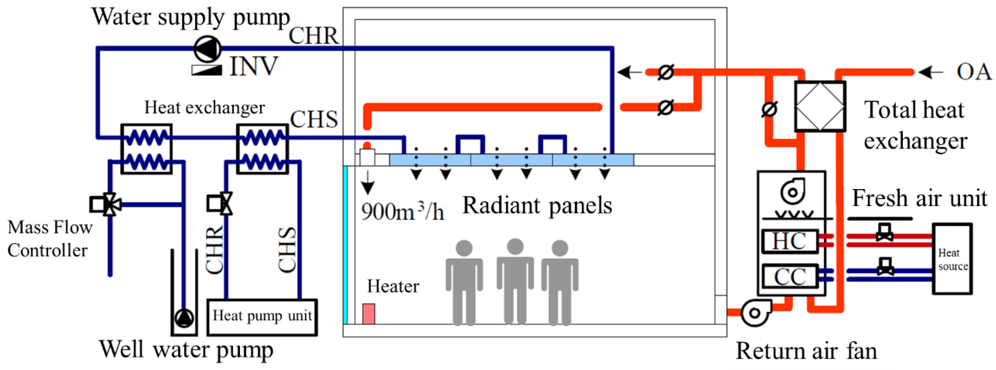
Figure 4 shows a schematic of the radiant air-conditioning system. The system included a radiant air conditioning system that handled the indoor sensible heat load, and a fresh air system that handled the indoor latent heat load. The cold and heat sources adopted a series system of a commonly used air source heat pump unit and well water, with a temperature that was maintained at 16 °C all year round as the cold water source; the cooling capacity of the unit was 20 kW. During cooling, the cold water source was preferentially used to cool the chilled water, and then sent to the coil of the radiation unit for cooling. When the cooling capacity was insufficient, the heat pump was switched on to supplement the cooling capacity. The water supply pump of the radiant panels was equipped with a flow controller, and the maximum flow rate was 35 L/min. The fresh air system consisted of a fresh air unit, total heat exchanger, and return fan. In the total heat exchanger, the indoor return air and fresh air were fully heat exchanged. On the one hand, the humidity of the fresh air could be adjusted; on the other hand, the fresh air could be precooled or preheated to reduce the energy consumption of the system. The return fan ran during the start-up phase of the system, and stopped after the indoor thermal environment became stable. At that time, fresh air entered the room from the tuyere on the enclosure structure, in order to keep the indoor air clean and the air pressure stable.
3. Establishment and Verification of Simplified Load Prediction Model for HVAC System
3.1. Mathematical Model
The mathematical model of the HVAC system load prediction included the load caused by the heat gain of the non-transparent building envelope, the load caused by the heat gain of the transparent building envelope, and the load caused by the infiltration heat gain. The convective heat gain was directly converted into the instantaneous load of the air conditioner, and the radiant heat gain was absorbed by the indoor wall, and gradually released to become the instantaneous cooling load. The air conditioning load calculation adopted the state–space method. The relevant assumptions made for the model were as follows: the solar heat gain entering the room through the glass was completely absorbed by the floor slab; the long-wave radiation heat gain varied with the change in the outer surface temperature of the envelope; the short-wave transmittance of the glass varied with the incident angle of the sun; and the thermal conductivity and convective heat transfer coefficient of the envelope were constant.
The current model presented hereafter was defined with typical assumptions used in common simulation tools. The model used one-dimensional component models of walls and windows. In this model, corresponding meshes, wall layers, and insulation position were specified. The components accounted for conductive heat transfers between inner computation nodes, convective heat transfers with the ambient air, and radiant heat transfers for the short-and long-wave radiation. As commonly used, the conductive and convective heat transfer coefficients were assumed to be constant, but the long-wave heat transfer coefficient was variable as a function of temperatures of concerned bodies. The window model included the solar transmittance calculation using variable transmittance rates as a function of the solar incident angle. In addition, the model considered heat loss through ventilation using a constant air change rate.
A model based on the shape characteristics of the laboratory was developed. For a laboratory with n different orientations (including walls and roofs in all directions), the corresponding model had to define 3n parameters related to the solar radiation. That is, each orientation included the amount of direct solar radiation per unit area , the amount of scattered radiation per unit area of the sky , and the cosine value of the incident angle of the sun cos i. The input parameters of the model included hourly outdoor air temperature Ta, hourly effective sky temperature Tsky, and hourly air conditioning load P. The equation of state of the mathematical model can be expressed as follows:
where C represents the material specific heat capacity and material density of each temperature node, which is a constant parameter, and matrices A and B include the heat transfer coefficients of the walls, windows, and other envelope structures. They also include parameters that vary with the temperature as a function of the nodal temperature. These were used to calculate the long-wave radiation heat gain matrices. B also includes time-varying parameters, such as the solar short-wave transmittance of the glass; represents the derivative with respect to time; T represents the temperature of each node (including walls, windows, floors, etc.); U represents the input parameters of the model (including outdoor air temperature, effective sky temperature, direct solar heat gain, sky scattered heat gain, and other external disturbances); Y represents the output parameter, which is the indoor air temperature in this model; and matrices J and D are constant and related to thermal parameters such as the thermal conductivity of the material [28].
3.2. Simplified Model (SM)
Since the order-reduction method used in the model can only be used for linear time-invariant systems, matrices A, B, C, D, and J in Equation (1) must be transformed into a constant time-invariant system [28]. The equation for calculating the long-wave radiation heat gain is as follows:
where ε represents the absorption rate of the outer wall, Fsky represents the angular coefficient of the wall-to-sky, represents the Stephen Boltzmann constant, and Ts represents the surface temperature of the outer wall. The nonlinear long-wave radiation heat gain calculation was linearly simplified, and the commonly used annual average effective sky temperature and annual average external wall surface temperature were used instead, so that was constant, which transformed matrices A(T) and B(T,t) into A and B(t).
When calculating the solar heat gain through the glass, the relationship between the solar shortwave transmittance and the angle of incidence of the sun relative to the normal to the glass was also nonlinear. In order to simplify the model, the heat gain from solar shortwave radiation per unit area was extracted and calculated separately in the preprocessing stage, and the solar heat gain through the glass was calculated separately using the transmittance that changes with the incident angle of the sun. The calculation equation is as follows:
where represents the weighted arithmetic mean of the insolation heat gain through all glass (W/m2), represents the time-varying direct radiation transmittance, represents the constant scattered radiation transmittance, represents the area facing each window facing i (m2), and and represent the direct and scattered radiation intensities (W/m2), respectively. was used as the input parameter for the model. In the model calculation, this parameter was multiplied by the total area of the window glass to obtain the total solar heat gain through the glass. It was assumed that the heat gain was absorbed by the floor slab. Through the above process, the model was transformed into a linear time-invariant system.
An equivalent envelope model was used to simplify the model further. By averaging the radiation intensities received by the walls and windows facing different directions in the model, the average radiation intensity of the wall and average radiation intensity of the window were obtained as input parameters for the simplified model. After this simplification, only one equivalent single wall and window could be used to simulate various complex architectural forms in the detailed model, significantly simplifying the input parameters for the model. The research behind describing complex and changeable architectural forms and simplifying models was included in the preprocessing process. Thus, the feedback parameters of the complex actual control process of the HVAC system were aggregated into equivalent single wall and window parameters.
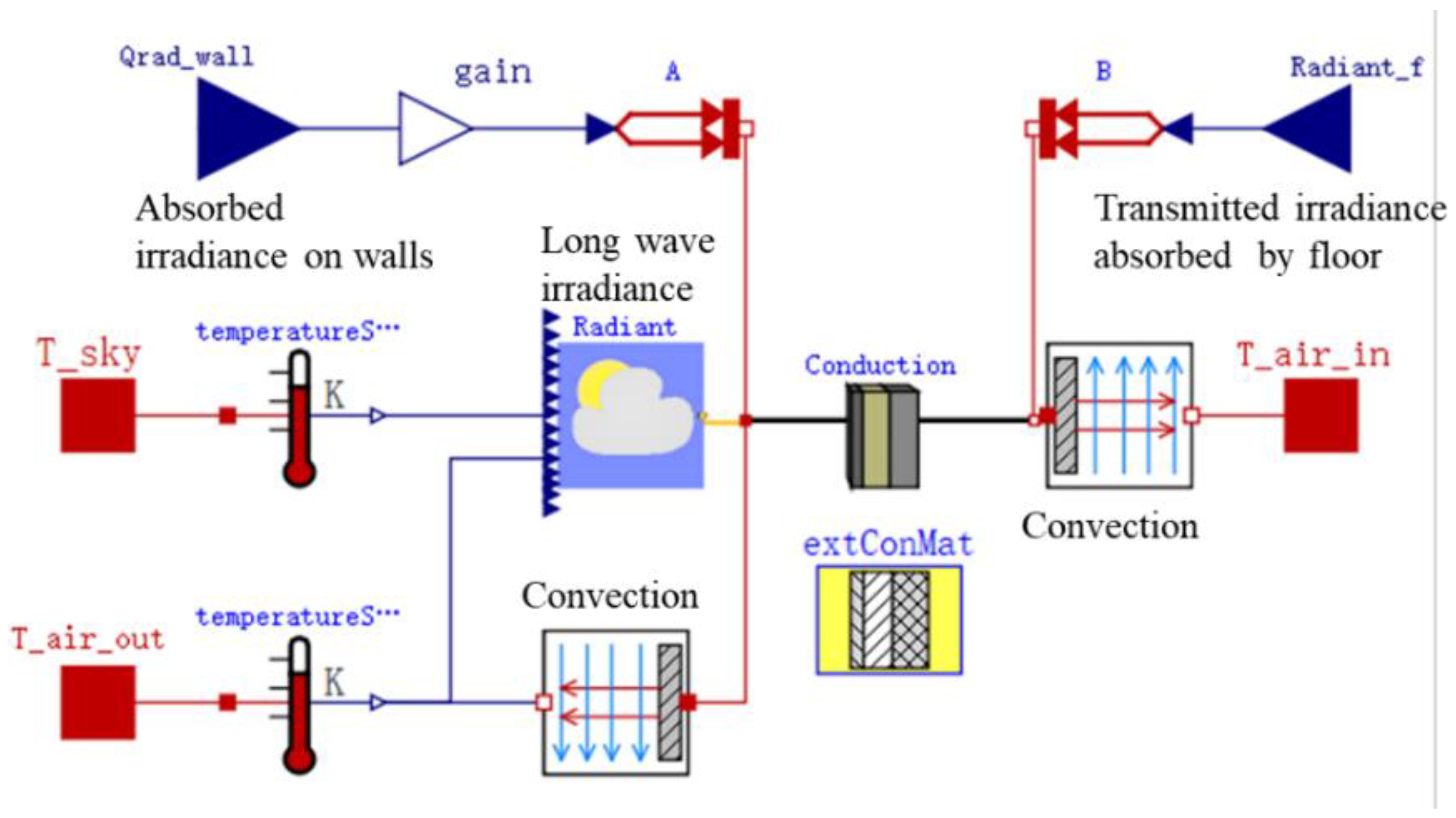
OpenModelica is an open-source Modelica-based modeling and simulation environment that is intended for industrial and academic applications [28]. It has the characteristics of parameterization, modularization, and graphics in Modelica language, so that system modules can be established independently, and quickly assembled. In this study, we used the building heat transfer module in the Buildings Library model library, and established a weather data reading module and building preprocessing module to build a simplified model for air conditioning system load forecasting. On this basis, a reduced-order model was established to improve model performance and calculation speed. We used this platform to establish a simplified numerical model, and to model the four main components of the wall, window, floor, and air. Figure 5 shows the wall as an example of a numerical model of the air-conditioning load caused by the heat gain of the wall. The heat gain on the outer surface of the wall includes long-wave radiation, solar radiation, convective heat exchange between the wall, atmosphere, and surrounding environment. These factors transfer outdoor heat to the inner surface of the wall through heat conduction; part of the heat is transferred to the indoor air in the form of convection, forming an instantaneous load, and the other part of the heat is in the form of long-wave radiation, assuming that it is completely absorbed by the floor.
We used basic building components under the OpenModelica platform to create wall, window, air, and floor modules. The air module considered the interior space of the entire building as a whole, separated from the outside world by walls and windows, and considered the heat storage capacity of the indoor air. Simultaneously, a ventilation rate parameter was introduced to consider the effects of air infiltration and natural ventilation. Finally, by assembling the modules, a simplified numerical model was obtained, as shown in Figure 6.
3.3. Reduced-Order Model (RM)
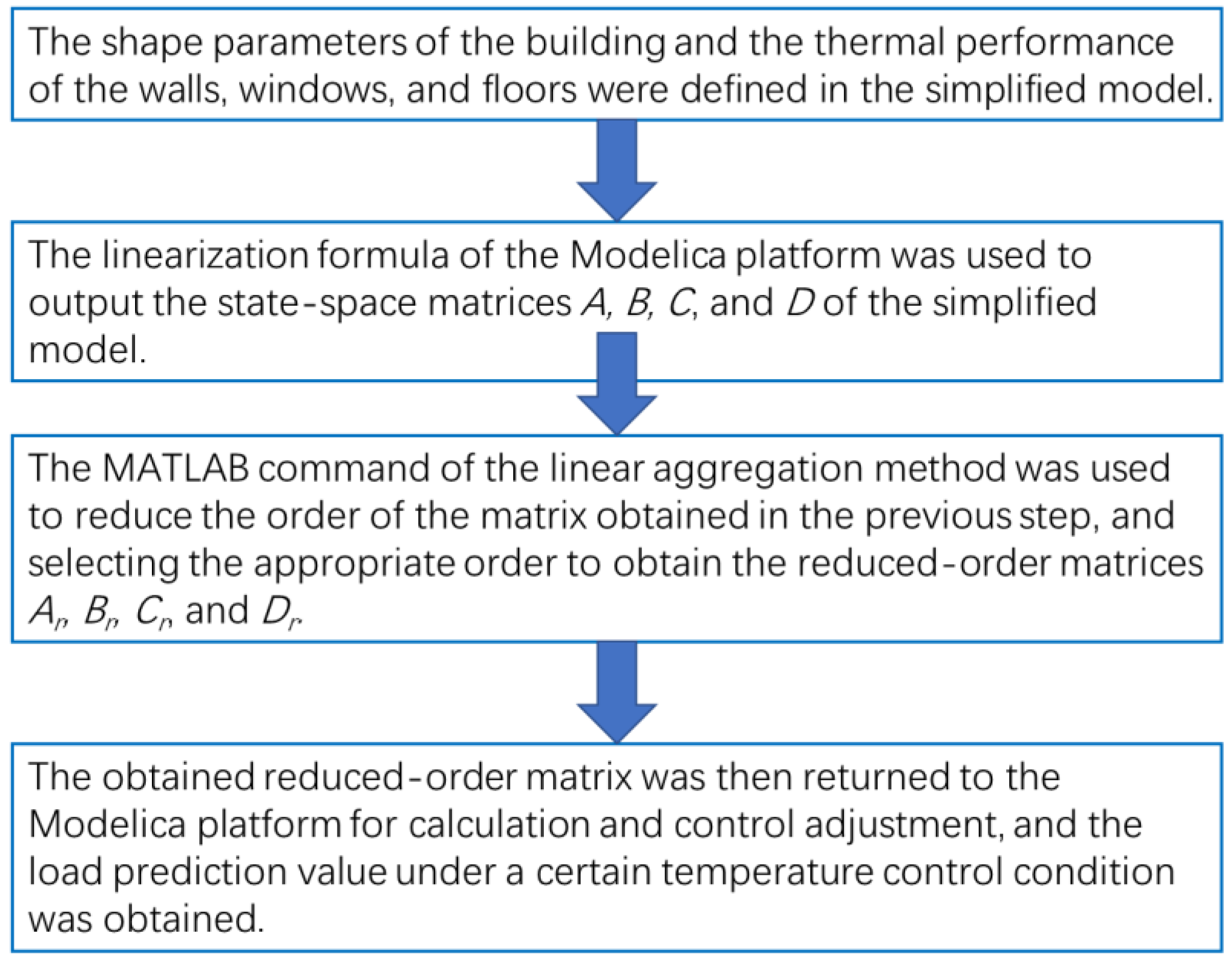
Based on the simplified model, a reduced-order model was established using the reduced-order method [29]. The order-reduction method uses mathematical means to transform the original model from high-order to low-order, from complex to simple, and to ensure that the simplified model output can approximate the mathematical processing of the original model output. If a high-order process can be approximated by a low-order model, using the low-order approximation model to design the control system can significantly simplify the calculation process and improve calculation speed [30]. In this study, the linear aggregation method was used for order reduction in a simplified model [31]. Aggregation combines the state variables of a system and uses a smaller set of state variables to describe the system model [32]. In a reduced-order model, making a reasonable choice of the reduced order is crucial to model simplification. In this study, MATLAB programming was used to realize the linear aggregation method.
Obtaining a reduced-order model from a numerically reduced model requires the following steps, as shown in Figure 7.
The real-time load obtained by the real-time indoor air temperature was realized using a proportional-integral-derivative (PID) controller. This process comprised three parts: measurement, comparison, and execution. The actual value of the controlled variable was measured, which in this study was the target feedback parameter of the simplified model, i.e., the indoor radiation temperature. It was compared with the expected value, and this deviation was used to correct the system response and perform regulatory control.
3.4. Model Validation
In general, it was difficult to determine the optimal reduction order of the reduced-order model, because this parameter is related to the frequency of excitation and type of building. In this study, the second, fourth, sixth, and tenth orders were selected as the comparison objects, and the calculation results were compared with the indoor temperature measured at No. 15 measuring point on 5 June. The results are shown in Figure 8. It can be seen that the errors between the calculated results of all reduced-order models and the experimental data were less than 3%, indicating high accuracy. The second-order model had some instability in the descending stage, whereas the curves of the sixth-order and tenth-order models almost overlapped. These results are further explained in Table 2. It can be seen that the accuracy of the second-order model was 99.9697%, the accuracy of the fourth-order model was 99.9981%, and the accuracy of the sixth-order model was 99.9996%, which is very close to 100%. Considering that this model was relatively simple, the second-order accuracy is usually less than 99.99% for a slightly more complex architectural model; thus, the fourth-order reduced-order model was selected for the calculation.
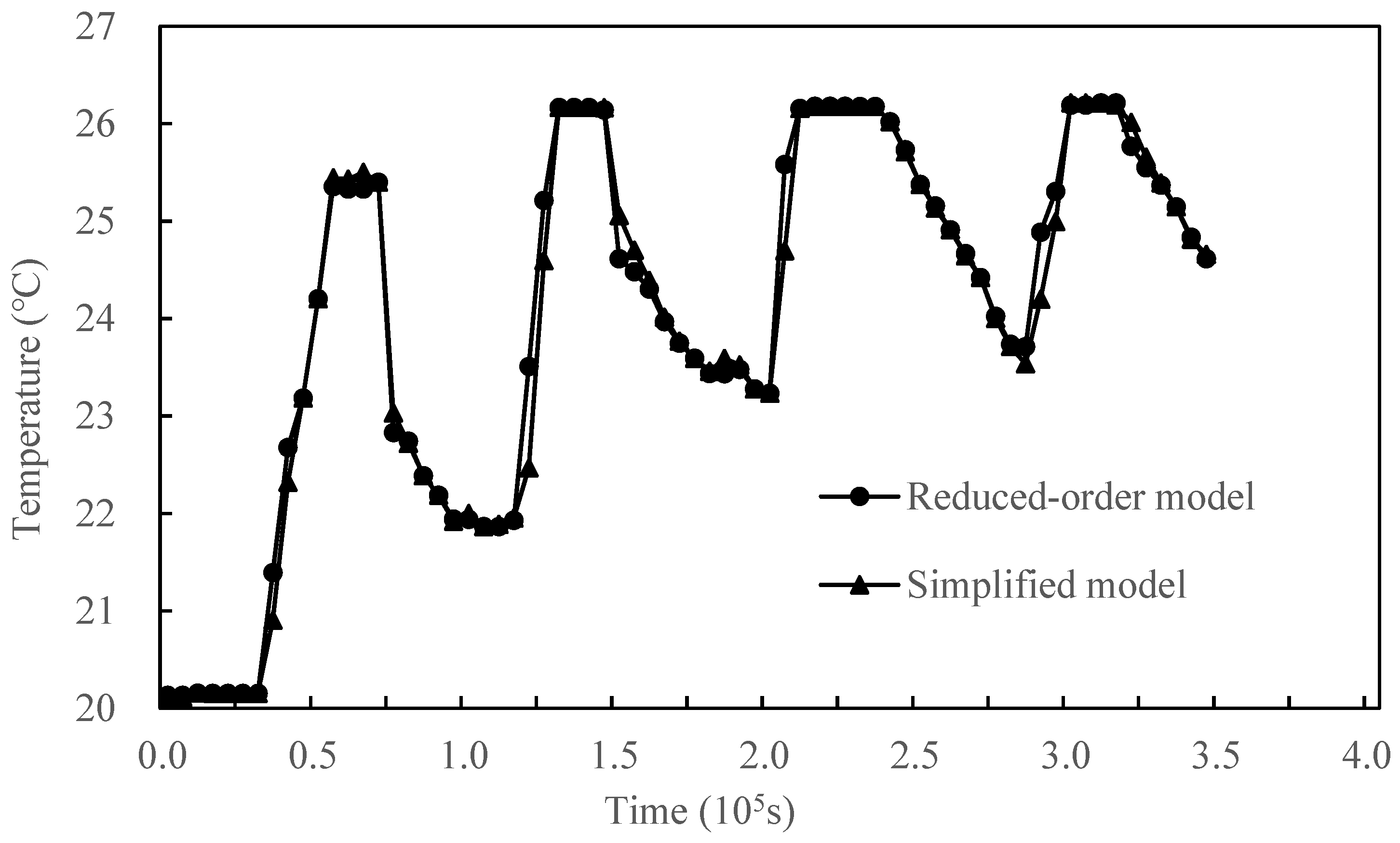
After determining the optimal order, the simplified model obtained in the previous section was used to verify the accuracy of the reduced-order model. Using the same meteorological preprocessing model, the reduced-order model was compared with the corresponding simplified model. Taking a set of tests as an example, the meteorological data for four days (1 June–4 June) were arbitrarily selected, and the indoor air temperature comparison chart shown in Figure 9 was obtained. The two curves are very close in the ascending stage, and the difference can be seen in the descending stage; the maximum temperature difference is only 0.33 °C. Figure 10 compares the load values predicted by the reduced-order and simplified models. It can be seen that the simulation results of the two models are very consistent. However, there is a large error in the initial stage because the initialization of the reduced-order model has no physical meaning, and there is no way to define the initial temperature. Equilibrium can only be gradually reached in the calculation.
4. Experimental Results and Discussion
4.1. Experimental Conditions
The target feedback parameter of the simplified model in this study was the mean indoor radiant temperature (MRT) [33]. For radiant air conditioning systems, the average radiant temperature has a faster response speed than the indoor air temperature. Radiant heat exchange accounts for 45% of the total heat exchange between the human body and the surrounding environment, and can better meet comfort requirements.
MRT can be obtained from the surface temperature of the indoor envelope structure. This method was adopted in this study. The calculation expression is as follows:
where represents the angle coefficient of surface i to surface j, and represents the surface temperature of surface j (°C).
This method did not require arranging the measurement points in the indoor personnel activity area. However, because of the large number of surfaces in an indoor envelope, it was necessary to arrange multiple measurement points for data collection. Therefore, the degree to which the determination of the envelope structure surface temperature could be simplified was crucial to the practicality of the system. Simplifying the MRT control system and reducing the number of sensors were important objectives of this study. The envelope structure surface temperature was measured using an Azbil TY7321B radiation temperature sensor with a range of 5–50 °C, and an accuracy of ±0.37 °C. In order to avoid affecting people walking indoors, the floor surface temperature was measured using thermocouples.
Figure 11 shows a schematic of the MRT control. The temperature and flow of the chilled water were fixed using the traditional constant-condition control method. MRT control monitors the temperature of the chilled water through the flow control valve on the cold and heat source side, or adjusts the flow rate of the chilled water through the frequency converter of the water pump to control the surface temperature of the radiant panel. In order to achieve the purpose of controlling the indoor MRT, control strategies can be divided into constant temperature and flow control strategies. The surface temperature of the radiant panel under the set MRT conditions was calculated by substituting the angle coefficient and temperature of each envelope structure into the radiant panel in Equation (4). Subsequently, based on the deviation between the current surface temperature of the radiant panel and the set value, the water temperature or flow rate of the radiant coil was controlled. The fresh air system adjusted the working conditions of the chilled water, and the humidifier sent air to the fresh air unit based on the set indoor humidity.
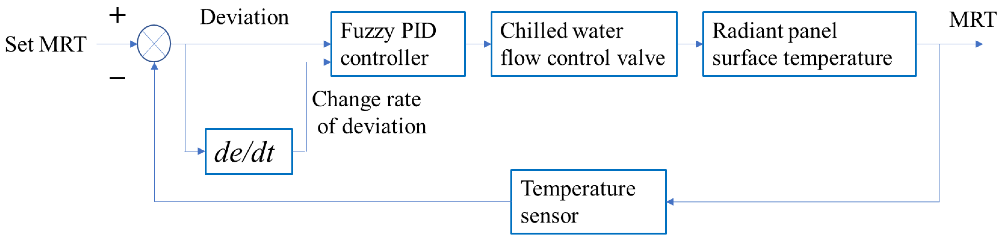
In the radiant air conditioner plus independent fresh air system as the controlled object, fuzzy PID (proportional-integral-derivative) control, which is common in HVAC systems [34,35], was used. The surface temperature of the radiant panel was controlled by adjusting the opening of the chilled water flow control valve, so that the MRT was consistent with the set value; the air supply volume was adjusted by controlling the fan inverter, so that the indoor fresh air volume and humidity were consistent with the set value. Taking the specific control process of the surface temperature of the radiant panel as an example, when the calculated MRT value deviated from the set value, the opening of the chilled water valve was controlled by changing the voltage, thereby adjusting the chilled water flow. The heat exchange between the radiant panel and the chilled water was changed to adjust the surface temperature of the radiant panel. The radiant heat exchange between the radiant panel and the indoor environment was changed to adjust the temperature of the air-conditioned room. The voltage adjustment range was 0–10 V, the linear corresponding temperature change range was 0–100 °C, and the frequency change range of the inverter was 0–50 Hz. The fuzzy PID control system is shown in Figure 12.
The experiment was carried out under the cooling conditions of an HVAC system, and the target MRT value was 26 °C. When using constant working condition control, the temperature of chilled water was fixed at 18 °C, and the flow rate was fixed at 35 L/min. When a constant flow control was used, the chilled water flow was fixed at 17.5 L/min. In order to prevent condensation on the radiant panel, the lower limit of the chilled water temperature was set to 14 °C. When using constant temperature control, the temperature of the chilled water was fixed at 16 °C, and the flow rate was varied between 0–35 L/min. The operating conditions of the three control methods were selected in the morning, with strong sunshine and high temperatures. In the afternoon, it was a cloudy day, and the temperature continued to decrease, causing significant changes in the air conditioning load.
4.2. Experimental Results and Discussion
Figure 13, Figure 14 and Figure 15 show the changes in the MRT, indoor temperature, and radiant panel surface temperature with time under different control methods. Figure 12 shows the change process for each temperature under constant working conditions. Before the start of the air conditioning system in the morning, as the outdoor air temperature gradually increased, both the indoor air temperature and the MRT increased to 31 °C. After the air conditioning system was started, the temperature of the radiant panel dropped rapidly, and the indoor air temperature and MRT gradually decreased and stabilized under the action of radiation and convection heat transfer. After 13:00, the outdoor temperature continued to increase to 30 °C, and the temperature difference with the highest temperature reached 4 °C. Since the chilled water flow and temperature remained unchanged, the cooling capacity provided by the air conditioning system was excessive, resulting in a continual decrease in the indoor air temperature and MRT. It can be seen that during the entire change process of the indoor air temperature and MRT, the indoor air temperature could also drop rapidly due to the forced convection of the mixed wind when the air conditioning system activated. However, after the indoor thermal environment stabilized, the load changed, the MRT continued to decrease, and the indoor temperature remained unchanged. When the outdoor temperature dropped significantly in the afternoon, the indoor temperature dropped from 27 °C to 26 °C between 13:00 and 18:00. The MRT decreased from 27 °C to 25 °C, and the magnitude and speed of the decline were greater than the indoor air temperature. This occurred mainly because the surface temperature of the east outer wall, which was in contact with the outdoor environment, was directly affected by the decrease in outdoor air temperature. Since the heat exchange with the outdoor environment was reduced, the surface temperature of the east outer wall decreased accordingly. Although constant operating condition control cannot maintain the indoor thermal environment when the air conditioning load changes significantly, the experimental results indicate that the MRT response to load changes was greater than the indoor air temperature under the same conditions. The air conditioning system can be adjusted in a timely manner for load changes using the MRT as a control parameter to feed back to the control system.
Figure 14 shows the variation process for each temperature under constant flow control. After the HVAC system was activated, the MRT and indoor air temperature gradually decreased and then stabilized. In the morning, the outdoor air temperature fluctuated to a certain extent, and the MRT responded and fed this back to the control system in order to control the indoor air temperature by adjusting the temperature of the chilled water. Although the indoor temperature also fluctuated, the amplitude was less than 0.5 °C. Between 13:00 and 14:00 in the afternoon, the outdoor temperature fluctuated rapidly, dropping by 2 °C within 10 min, and then rising by 2 °C within 10 min after being constant for approximately an hour. It can be seen that during this process, the MRT decreased significantly, and the corresponding increase in the temperature of the chilled water increased the temperature of the radiant panel. The indoor temperature also fluctuated, but the amplitude was controlled within 0.3 °C, which did not affect indoor comfort. Throughout the entire process, the indoor air temperature remained stable, with the fluctuation range being much smaller than that of the MRT and the surface temperature of the radiant panel.
Figure 15 shows the changing process for each temperature under the constant temperature control. The variation law of each temperature under this control method in the morning was similar to that under constant flow control; however, there was a large difference in the afternoon. In the afternoon, the outdoor temperature continued to decrease, and the indoor air conditioning load gradually decreased. The surface temperature of the radiant panel gradually decreased to 20 °C after the system was activated. After 14:00, it fluctuated between 21–23 °C as the outdoor temperature gradually decreased, and the affected MRT fluctuated between 25.5–26 °C. It can be seen that under constant temperature control, the system responded in a timely manner to changes in the air conditioning load; however, when the load was small, the system adjusted the board temperature by starting and stopping. In addition, similarly to the constant flow control condition, after 13:00 the MRT and surface temperature of the radiant panel fluctuated with time, but the variation in the indoor temperature was not large. It can be observed that the response speed of the indoor air temperature to the surface temperature of the radiant panel was slow. This helped to maintain thermal stability in the room; however, care must be taken to prevent excessive cooling of the radiant panels to cause condensation.
Figure 16 shows the horizontal distribution of MRT under constant flow control after the indoor thermal environment was stabilized. The MRT in the central area of the room was 26 °C, and near the enclosure it was 26.5–27.5 °C, with the highest at the east outer wall. It can be observed that the distribution and change in indoor air conditioning load had a significant influence on the MRT. If there are no measures implemented, such as thermal insulation treatment for the enclosure structure and for the east outer wall, which are greatly affected by the environment, special treatment needs to be taken when applying the MRT control method.
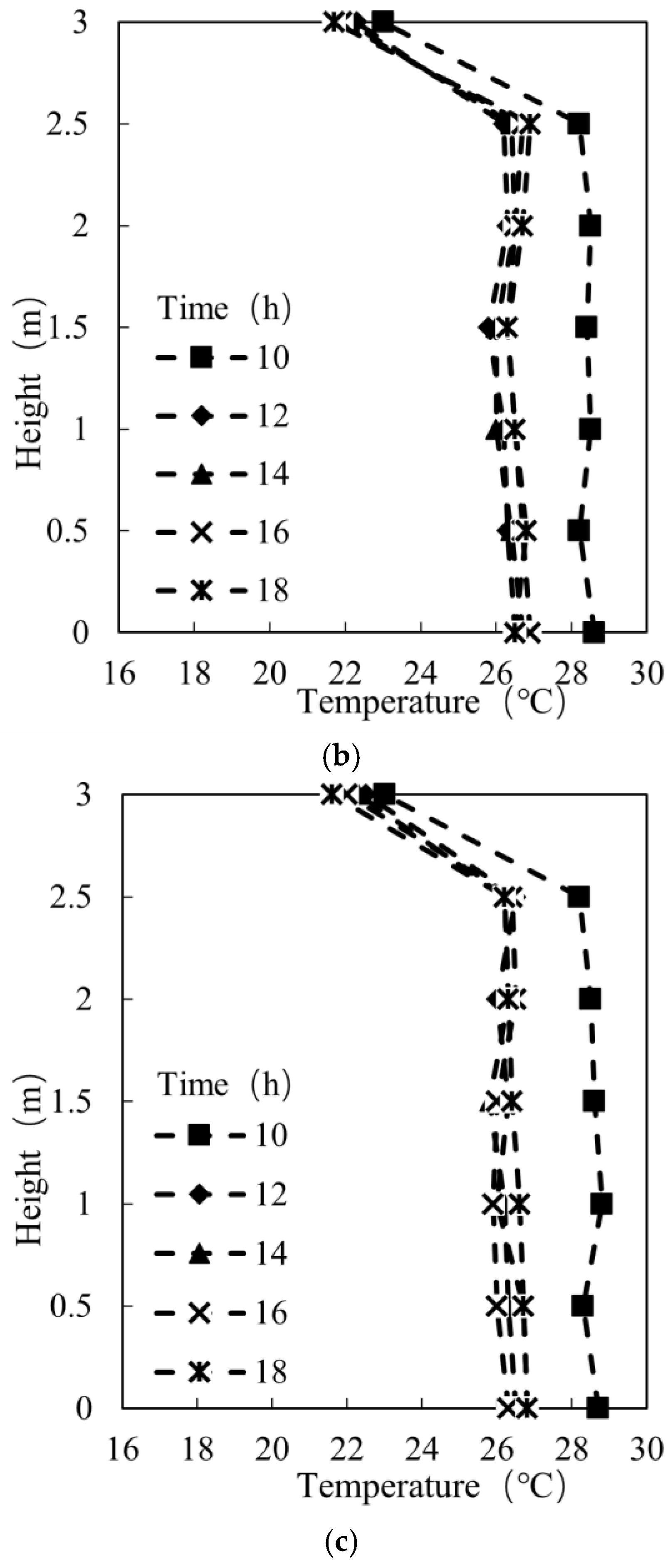
Figure 17 shows the temperature distribution in the vertical direction for the three control methods. It can be observed that the vertical temperature difference in the working area did not exceed 1 °C, and that the three control methods produced a uniform indoor thermal environment.
4.3. Simplified System Results and Discussion
From the experimental results in Section 4.2, it can be observed that controlling the indoor average radiation temperature as the target feedback parameter of the simplified model can maintain a stable indoor thermal environment and respond well to the distribution and changes in the air conditioning load. However, this control strategy requires the installation of sensors on the surfaces of each indoor enclosure to collect the surface temperature. The control system is complicated and costly; therefore, considerations can be made to simplify the system further. The specific method is to study the relationship between the surface temperature of each envelope and the indoor air temperature, and replace the measured data with the calculation results of the prediction model, thereby reducing the number of radiation temperature sensors.
Figure 18 shows the relationship between the indoor air temperature tair and the surface temperature of each envelope tw when the air conditioning system is activated in the summer. It can be seen that the relationship between the surface temperature and indoor air temperature of the east outer wall was not very obvious, owing to the influences of solar radiation and the outdoor environment. However, there was a good linear relationship between the surface temperature of the south inner wall, west inner wall, and north inner wall, with the indoor air temperature. From this, an approximate relationship between the indoor air temperature and inner surface temperature of the envelope was obtained, as follows:
where represents the inner surface temperature of the envelope (°C), and represents the indoor air temperature (°C).
Table 3 presents the coefficients of the surface temperature prediction models for the southern, western, and northern interior walls. It can be seen that the surface temperature of each inner wall was not much different from the indoor air temperature.
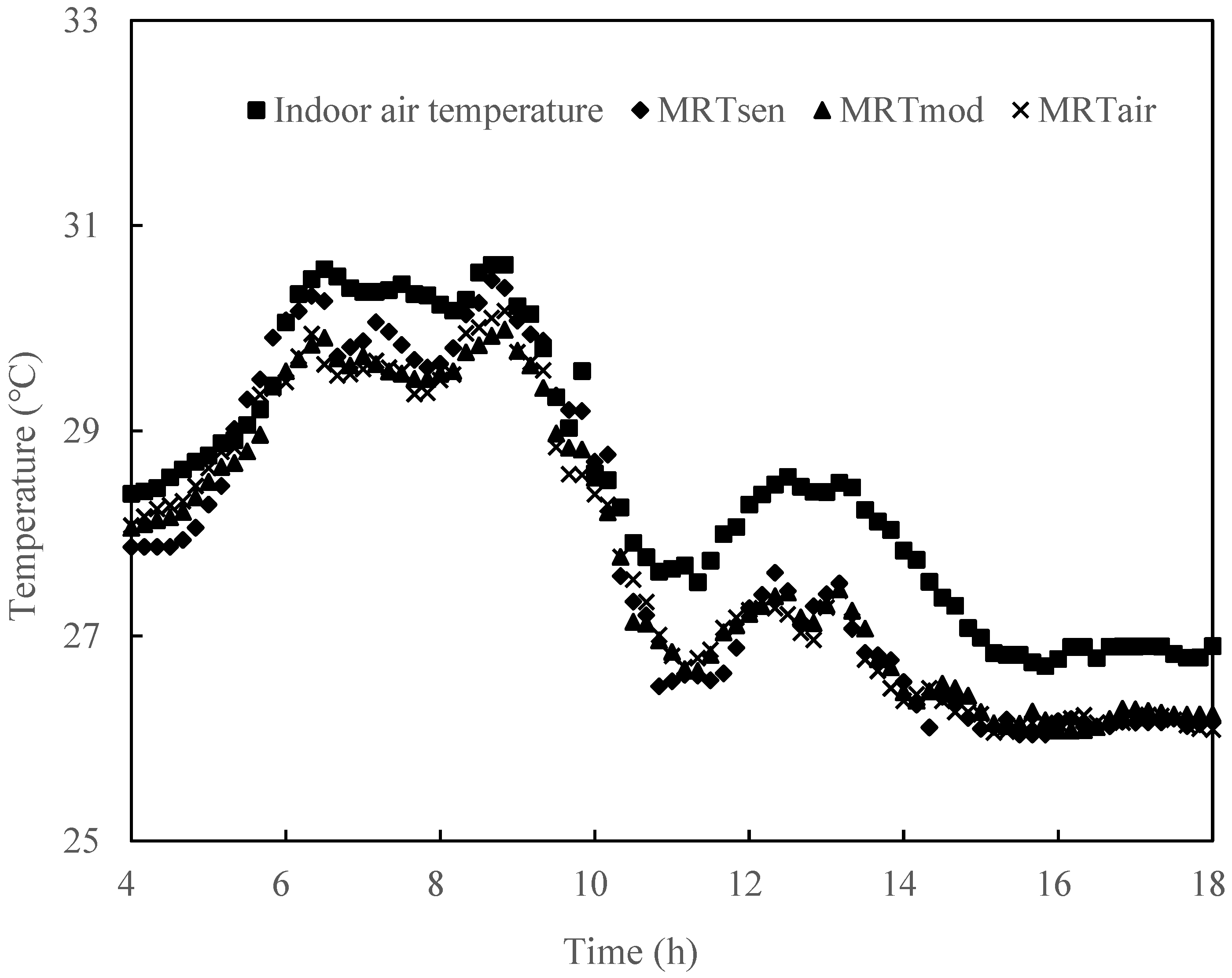
The angle coefficients of each enclosure structure where the feedback signal collection point was located were all less than 0.16. Therefore, when the surface temperature of the envelope structure is not significantly different from the indoor air temperature, it is assumed that the surface temperature of the envelope structure is equal to the indoor air temperature, and will not have a significant influence on the accuracy of the MRT prediction. Except for the surface temperature of the floor with a large angle coefficient, for the east outer wall that is greatly affected by solar radiation, and the surface temperature of the ceiling that is greatly affected by the air conditioning system, the MRT calculated by the prediction model for the surface temperature of other envelope structures was recorded as MRTmod. When the surface temperatures of other envelope structures were regarded as equal to the indoor air temperature, the MRT was recorded as MRTair. When all envelope surface temperatures were measured by sensors, the MRT was recorded as MRTsen. Figure 19 shows a comparison of the results obtained using the three MRT calculation methods. It can be seen that at 6:00, 9:00 and 11:00, the indoor air temperature varied greatly. MRTair failed to reflect the inertia of indoor air temperature change over time, which was 0.5 °C different from MRTsen. During the stabilization process at each temperature, the difference between MRTmod and MRTsen did not exceed 0.2 °C, which is closer to the measured results than MRTair, showing higher accuracy. Overall, there was little difference between the three MRT results; the change trend and process were consistent, and the error was less than 5%. It can be seen that it is feasible to establish an MRT prediction model to simplify the calculation method for the control system.
5. Conclusions
This study used the open-source Buildings Library model library developed by Lawrence Berkeley National Laboratory to establish a load prediction control model of a building dynamic HVAC system, using the open-source Modelica-based Building Library. The linear aggregation method was used to establish a reduced-order model. The accuracy of the simplified and reduced-order models was verified. The establishment of a simplified prediction model for building a dynamic HVAC system load significantly reduces the required input parameters; moreover, these parameters are the most basic of building design, and are easily measured environmental parameters. This can overcome the difficulty of obtaining detailed building parameters during the regional planning stage. Simultaneously, a reduced-order model was used to calculate the annual load prediction of the building, which can improve the calculation speed of the simulation and control process. A control strategy was constructed using the indoor average radiant temperature aggregated by the simplified prediction model of the HVAC system load as the target feedback parameter, and its feasibility was verified experimentally. It was found that MRT can predict changes in outdoor air temperature and load over time, effectively reducing the influence of load changes in addition to maintaining the stability of the indoor thermal environment. However, in the case of constant temperature control, the system was adjusted by starting and stopping when the load was small. Therefore, the ideal control strategy is to use constant temperature control to improve the response speed when the load and its variation are large, and to respond more accurately to load changes by constant flow control when the load is small. The MRT calculation method was further simplified based on model predictive control, and experimental verification was performed. It was found that the simplified model could reflect the change law in time when the indoor temperature varied significantly; the error was less than 5%, and the change trends and processes were consistent. This study provides reference and engineering experience for the practical application of a dynamic HVAC system load-simplified prediction model for building HVAC system control. In a follow-up study, the building internal disturbance module will be introduced to more accurately predict building HVAC system control. This study simplifies the load prediction model of a building’s dynamic HVAC system so that it can be applied to the actual construction and operation of HVAC control systems. However, instead of simply reducing the model and control accuracy, the main research workload is placed into the design stage of the entire building, including the HVAC system; the key parameters are screened and optimized based on the determination of various building characteristics.
Author Contributions
Conceptualization, J.W. and Q.S.; methodology, Q.S. and H.C.; investigation, J.W. and Q.S.; resources, Y.L.; data curation, Y.L.; writing—original draft preparation, Q.S. and Y.L.; writing—review and editing, J.W. and Q.S.; supervision, Q.S. and H.C.; project administration, Q.S. and H.C. All authors have read and agreed to the published version of the manuscript.
Funding
This research was funded by the National Key Research and Development Program of China, grant number 2016YFC0700303, and the Natural science research project of colleges and universities in Jiangsu Province, grant number 19KJD560001.
Institutional Review Board Statement
Not applicable.
Informed Consent Statement
Not applicable.
Data Availability Statement
Not applicable.
Conflicts of Interest
The authors declare no conflict of interest.
References
- Zhang, X.D.; Liu, S.S. Analysis of key points of energy saving assessment on civil buildings. Build. Energy Effic. 2014, 42, 81–84. [Google Scholar]
- Cho, J.; Kim, Y.; Koo, J. Energy-cost analysis of HVAC system for office buildings: Development of a multiple prediction methodology for HVAC system cost estimation. Energy Build. 2018, 173, 562–576. [Google Scholar] [CrossRef]
- Yang, Z. Development and application prospect of cool storage. J. HVAC 2010, 10, 261–263. [Google Scholar]
- Ren, C.; Cao, S. Implementation and visualization of artificial intelligent ventilation control system using fast prediction models and limited monitoring data. Sustain. Cities Soc. 2020, 52, 101860. [Google Scholar] [CrossRef]
- Yang, H.; Jia, L.; Yang, L.X. CFD Simulation on Tunnel Fire Smoke Control in Beijing Metro the 4th Line. Build. Sci. 2009, 25, 98–104. [Google Scholar]
- Xiong, C.Y.; Sun, Z.; Meng, Q.L.; Li, Z.Y.; Wei, Y.G.; Zhao, F. A simplified improved transactive control of air-conditioning demand response for determining room set-point temperature: Experimental studies. Appl. Energy 2022, 323, 119521. [Google Scholar] [CrossRef]
- Li, X.M.; Zhang, C.; Zhao, T.Y.; Han, Z.W. Adaptive predictive control method for improving control stability of air-conditioning terminal in public buildings. Energy Build. 2021, 249, 111261. [Google Scholar] [CrossRef]
- Yang, S.Y.; Wan, M.P.; Ng, B.F.; Dubey, S.; Henze, G.P.; Chen, W.Y.; Baskaran, K. Experimental study of model predictive control for an air-conditioning system with dedicated outdoor air system. Appl. Energy 2020, 257, 113920. [Google Scholar] [CrossRef]
- Zhao, N.; Gorbachev, S.; Yue, D.; Kuzin, V.; Dou, C.X.; Zhou, X.; Dai, J.F. Model predictive based frequency control of power system incorporating air-conditioning loads with communication delay. Int. J. Electr. Power Energy Syst. 2022, 138, 107856. [Google Scholar] [CrossRef]
- Lei, L.; Liu, W. Predictive control of multi-zone variable air volume air-conditioning system based on radial basis function neural network. Energy Build. 2022, 261, 111944. [Google Scholar] [CrossRef]
- Zhao, M.; Luo, X.L.; Kong, Q.X.; Yu, B.F. Simulation and analysis of influence of inlet parameters on temperature gradient of floor air distribution system. Refrig. Air-Cond. 2005, 5, 39–42. [Google Scholar]
- Georges, L.; Thalfeldt, M. Validation of a transient zonal model to predict the detailed indoor thermal environment: Case of electric radiators and wood stoves. Build. Environ. 2019, 149, 169–181. [Google Scholar] [CrossRef]
- Liu, W.; You, R.Y.; Zhang, J. Development of a fast fluid dynamics—based adjoint method for the inverse design of indoor environments. J. Build. Perform. Simul. 2017, 10, 326–343. [Google Scholar] [CrossRef]
- Ren, C.; Cao, S.J. Development and application of linear ventilation and temperature models for indoor environmental prediction and HVAC systems control. Sustain. Cities Soc. 2019, 51, 101673. [Google Scholar] [CrossRef]
- Zhang, W.R.; Hiyama, K.; Kato, S. Building energy simulation considering spatial temperature distribution for nonuniform indoor environment. Build. Environ. 2013, 63, 89–96. [Google Scholar] [CrossRef]
- Ma, Y.; Borrelli, F.; Hencey, B.; Coffey, B.; Bengea, S.; Haves, P. Model predictive control for the operation of building cooling systems. IEEE Trans. Control Syst. Technol. 2012, 20, 796–803. [Google Scholar]
- Široký, J.; Oldewurtel, F.; Cigler, J.; Prívara, S. Experimental analysis of model predictive control for an energy efficient building heating system. Appl. Energy 2011, 88, 3079–3087. [Google Scholar] [CrossRef]
- Chen, X.; Wang, Q.; Srebric, J. Occupant feedback based model predictive control for thermal comfort and energy optimization: A chamber experimental evaluation. Appl. Energy 2016, 164, 341–351. [Google Scholar] [CrossRef]
- Yang, S.; Wan, M.P.; Chen, W.; Ng, B.F.; Dubey, S. Model predictive control with adaptive machine-learning-based model for building energy efficiency and comfort optimization. Appl. Energy 2020, 271, 115147. [Google Scholar] [CrossRef]
- Ascione, F.; Bianco, N.; Stasio, C.; Mauro, G.M.; Vanoli, G.P. Simulation-based model predictive control by the multi-objective optimization of building energy performance and thermal comfort. Energy Build. 2016, 111, 131–144. [Google Scholar] [CrossRef]
- Castilla, M.; Álvarez, J.D.; Normey-Rico, J.E.; Rodríguez, F. Thermal comfort control using a non-linear MPC strategy: A real case of study in a bioclimatic building. J Process Control 2014, 24, 703–713. [Google Scholar] [CrossRef]
- Wang, L.Z.; Tan, H.W.; Wu, Y. Regional building cooling load prediction model based on Monte Carlo simulation. J. Cent. South Univ. (Sci. Technol.) 2014, 45, 4026. [Google Scholar]
- Lin, H.H.; Huang, J.T.; Wang, Y.W. Building combined cooling heat and power production system plan based on load curve and operation mode analysis. J. Shenyang Inst. Eng. (Nat. Sci.) 2010, 3, 193. [Google Scholar]
- Matthias, R.; Lin, A.C. Regional energy demand and adaptations to climate change: Methodology and application to the state of Maryland, USA. Energy Policy 2006, 34, 2820. [Google Scholar]
- Heiple, S.; Sailor, D.J. Using building energy simulation and geospatial modeling techniques to determine high resolution building sector energy consumption profiles. Energy Build. 2008, 40, 1426. [Google Scholar] [CrossRef] [Green Version]
- Deque, F.; Ollivier, F.; Poblador, A. Grey boxes used to represent buildings with a minimum number of geometric and thermal parameters. Energy Build. 2000, 31, 29. [Google Scholar] [CrossRef]
- Kim, E.J.; Plessis, G. Urban energy simulation: Simplification and reduction of building envelope models. Energy Build. 2014, 84, 193. [Google Scholar] [CrossRef]
- Shitahun, A.; Ruge, V.; Gebremedhin, M.; Bachmann, B.; Eriksson, L.; Andersson, J.; Diehl, M.; Fritzson, P. Model-Based Dynamic Optimization with OpenModelica and CasADi. IFAC Proc. Vol. 2013, 46, 446–451. [Google Scholar] [CrossRef]
- Palomo, E.; Bonnefous, Y.; Deque, F. Guidance for the selection of a reduction technique for thermal model. In Proceedings of the Building Simulation of International Building Performance Simulation Association, Prague, Czech Republic, 23 September 1997. [Google Scholar]
- Li, K.J. Modeling, Control and Optimization for Indoor Environment and Energy Consumption Prediction. Ph.D. Thesis, Zhejiang University, Hangzhou, China, 2013. [Google Scholar]
- Moore, B.C. Principal component analysis in linear system: Controllability, observability and model reduction. IEEE Trans. Autom. Control 1981, 26, 17. [Google Scholar] [CrossRef]
- Zhu, X.P.; Chen, S.L. A simple model order reduction method. J. Naniing Univ. Aeronaut. Astronaut. 1994, 26, 464. [Google Scholar]
- Mehmet, F.Ö.; Cihan, T. A comprehensive comparison and accuracy of different methods to obtain mean radiant temperature in indoor environment. Therm. Sci. Eng. Prog. 2022, 31, 101295. [Google Scholar]
- Xie, Y.; Yang, P.; Qian, Y.; Zhang, Y.; Li, K.; Zhou, Y. A two-layered eco-cooling control strategy for electric car air conditioning systems with integration of dynamic programming and fuzzy PID. Appl. Therm. Eng. 2022, 211, 118488. [Google Scholar] [CrossRef]
- Servet, S.; Mehmet, K.; Hasan, A. Design and simulation of self-tuning PID-type fuzzy adaptive control for an expert HVAC system. Expert Syst. Appl. 2009, 36, 4566–4573. [Google Scholar]
Figure 1.
Laboratory floor plan.

Figure 2.
Radiant unit.

Figure 3.
Layout of laboratory measuring points.

Figure 4.
Schematic diagram of radiant air conditioning system.

Figure 5.
Numerical simplified model for a wall.

Figure 6.
Numerical simplified model.

Figure 7.
Procedure used to obtain the RM model.

Figure 8.
Choice of reduction order.

Figure 9.
Indoor air temperature between the SM and RM for testing.

Figure 10.
Hourly load between the SM and RM.

Figure 11.
Schematic flow chart of the MRT control.

Figure 12.
The fuzzy PID control system.

Figure 13.
Variation process of MRT, indoor temperature, and surface temperature of radiant panel with time, under constant working conditions.
Figure 13.
Variation process of MRT, indoor temperature, and surface temperature of radiant panel with time, under constant working conditions.

Figure 14.
Variation process of MRT, indoor temperature, and surface temperature of radiant panel with time, under constant flow control.
Figure 14.
Variation process of MRT, indoor temperature, and surface temperature of radiant panel with time, under constant flow control.

Figure 15.
Variation process of MRT, indoor temperature, and surface temperature of radiant panel with time, under constant temperature control.
Figure 15.
Variation process of MRT, indoor temperature, and surface temperature of radiant panel with time, under constant temperature control.

Figure 16.
Horizontal distribution of MRT under constant flow control.

Figure 17.
Temperature distribution in the vertical direction. (a) Vertical temperature distribution under constant condition control; (b) vertical temperature distribution under constant flow control; (c) vertical temperature distribution under constant temperature control.
Figure 17.
Temperature distribution in the vertical direction. (a) Vertical temperature distribution under constant condition control; (b) vertical temperature distribution under constant flow control; (c) vertical temperature distribution under constant temperature control.


Figure 18.
Relationships between indoor air temperature and surface temperature of each envelope. (a) Linear fitting of the surface temperature of the eastern inner wall and indoor air temperature; (b) linear fitting of the surface temperature of the south inner wall and indoor air temperature; (c) linear fitting of the surface temperature of the west inner wall and indoor air temperature; (d) linear fitting of the surface temperature of the north inner wall and indoor air temperature.


Figure 19.
Comparison of the results obtained by the three MRT calculation methods.


Table 1.
Thermal parameters of the building envelope.
| Building Envelope | Structure | Thickness/m | Thermal Conductivity/ (W/m2⋅K) |
|---|---|---|---|
| Interior wall | Bricks, cement mortars | 0.600 | 1.106 |
| Exterior wall | Bricks, cement mortars | 0.550 | 1.281 |
| Partition wall | Gypsum board, extruded polystyrene foam | 0.050 | 1.025 |
| Exterior window | Normal glass, aluminum alloy frame | 0.006 | 6.400 |
| Ground floor | Damp-proof course layer, thermal insulating layer, fine aggregate concrete layer, cement screed layer | 0.300 | 1.515 |
| Floor slab | Fine aggregate concrete, reinforced concrete slab, thermal insulation mortar, anti-cracking gypsum + mesh + flexible putty | 0.200 | 2.136 |
Table 2.
Contribution of each order.
| Order | Contribution | Total Contribution | Order | Contribution | Total Contribution |
|---|---|---|---|---|---|
| 1 | 99.9421 | 99.9421 | 6 | 0.0005 | 99.9996 |
| 2 | 0.0281 | 99.9697 | 7 | 0.0003 | 99.9999 |
| 3 | 0.0182 | 99.9879 | 8 | 0.0000 | 100 |
| 4 | 0.0099 | 99.9981 | 9 | 0.0000 | 100 |
| 5 | 0.0009 | 99.9991 | 10 | 0.0000 | 100 |
Table 3.
Approximate coefficients for the surface temperature of the building envelope and the indoor air temperature.
Table 3.
Approximate coefficients for the surface temperature of the building envelope and the indoor air temperature.
| Building Envelope | a | b | R2 |
|---|---|---|---|
| South inner wall | 0.9678 | 1.5127 | 0.8155 |
| West inner wall | 0.9478 | 1.1899 | 0.9182 |
| North inner wall | 1.0928 | −2.3481 | 0.8114 |
Publisher’s Note: MDPI stays neutral with regard to jurisdictional claims in published maps and institutional affiliations. |
© 2022 by the authors. Licensee MDPI, Basel, Switzerland. This article is an open access article distributed under the terms and conditions of the Creative Commons Attribution (CC BY) license (https://creativecommons.org/licenses/by/4.0/).
Share and Cite
MDPI and ACS Style
Si, Q.; Wei, J.; Li, Y.; Cai, H. Optimization for the Model Predictive Control of Building HVAC System and Experimental Verification. Buildings 2022, 12, 1602. https://doi.org/10.3390/buildings12101602
AMA Style
Si Q, Wei J, Li Y, Cai H. Optimization for the Model Predictive Control of Building HVAC System and Experimental Verification. Buildings. 2022; 12(10):1602. https://doi.org/10.3390/buildings12101602
Chicago/Turabian StyleSi, Qiang, Jianjun Wei, Yuan Li, and Hao Cai. 2022. "Optimization for the Model Predictive Control of Building HVAC System and Experimental Verification" Buildings 12, no. 10: 1602. https://doi.org/10.3390/buildings12101602
Note that from the first issue of 2016, this journal uses article numbers instead of page numbers. See further details here.