
Research on a U-Net Bridge Crack Identification and Feature-Calculation Methods Based on a CBAM Attention Mechanism

Abstract
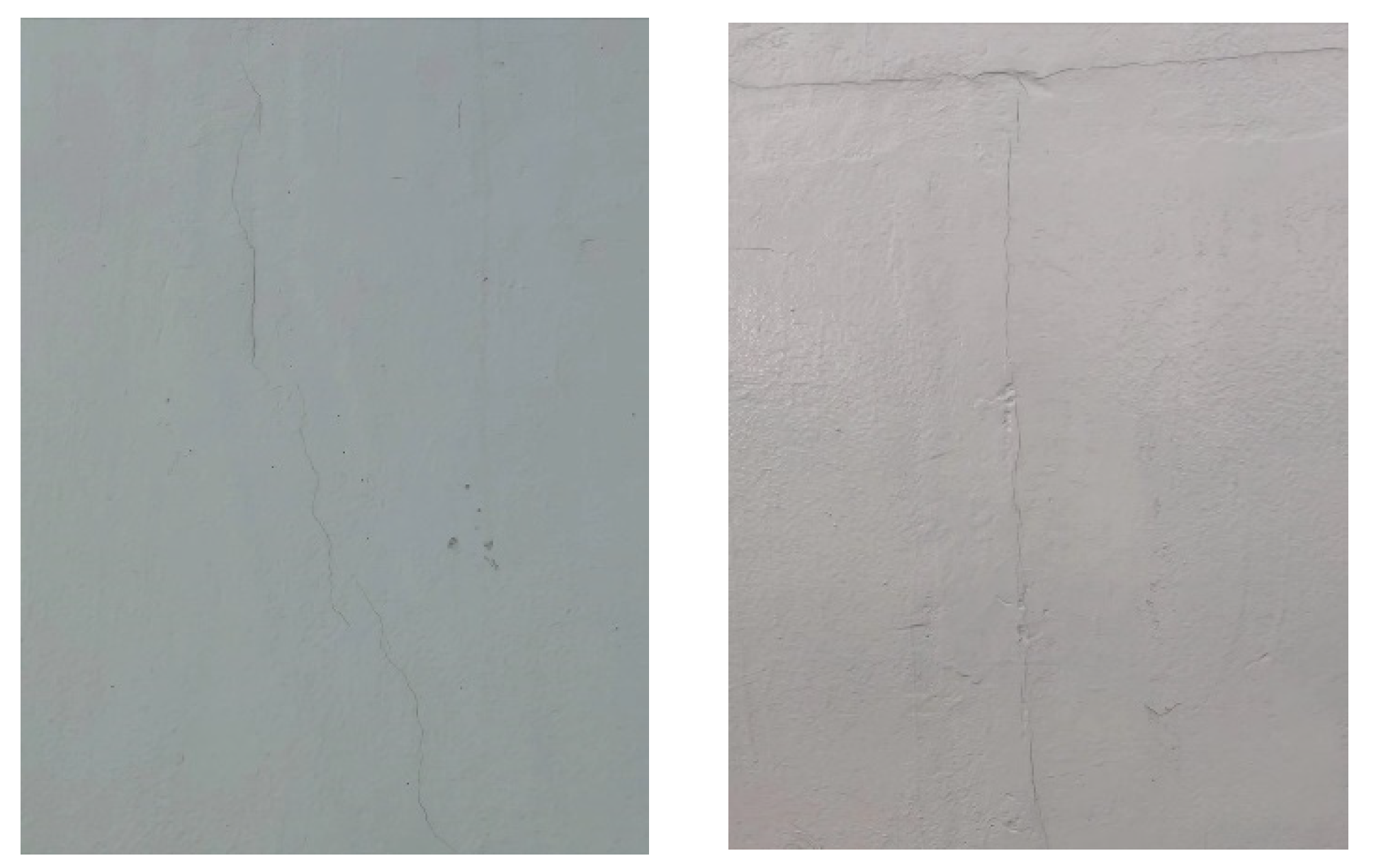
:1. Introduction
2. U-Net Methods and Channels, Spatial Attention Mechanisms
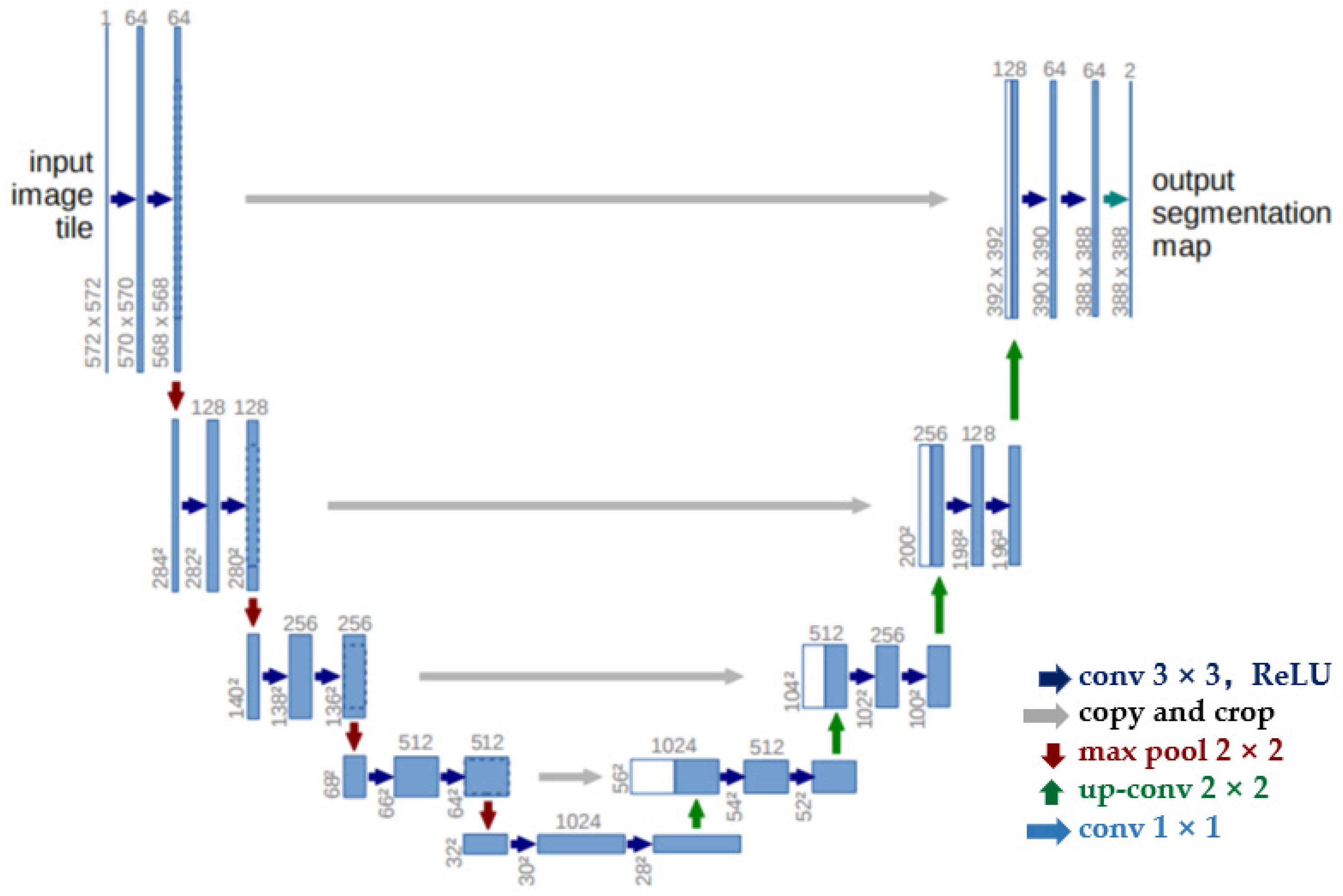
2.1. U-Net
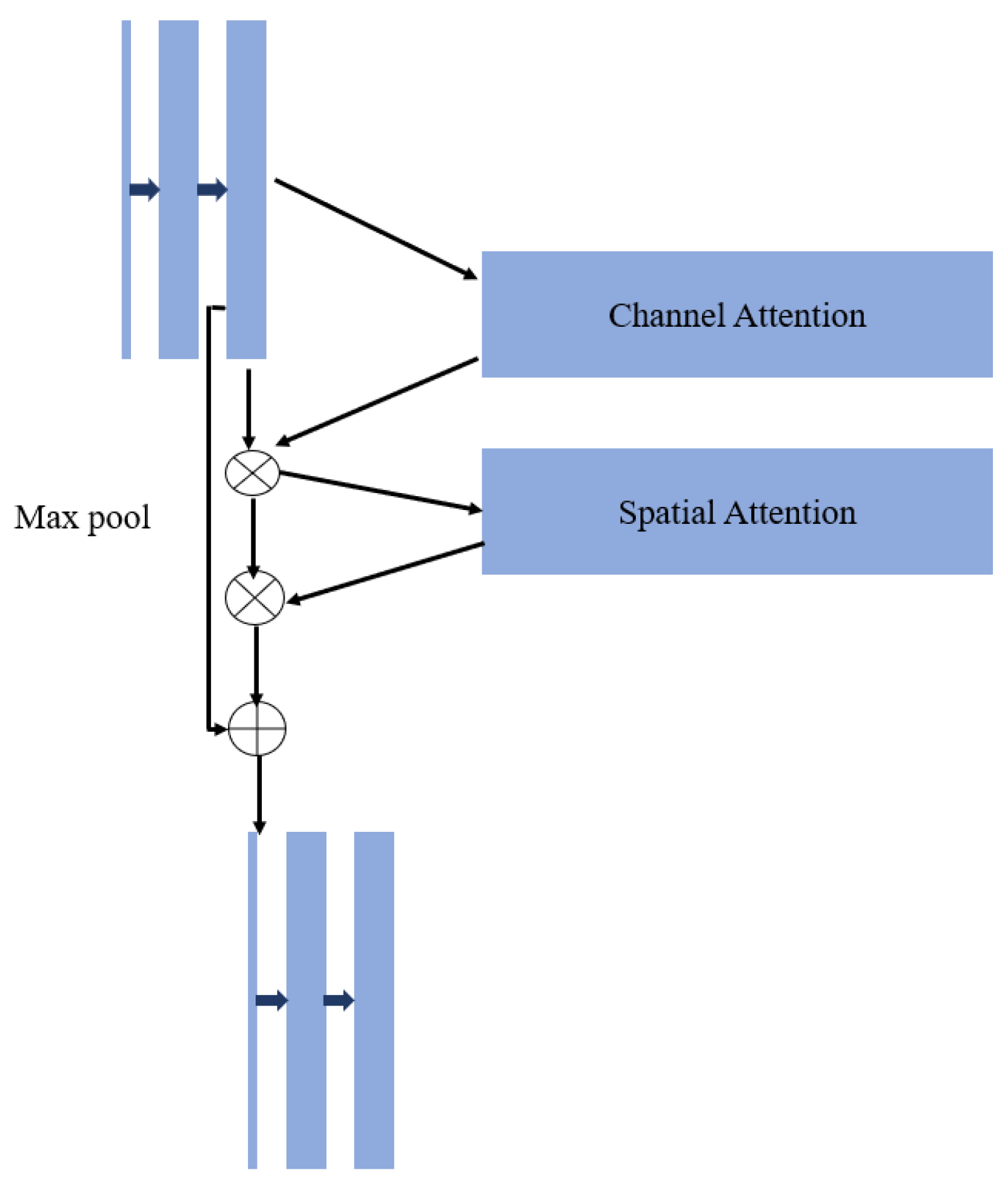
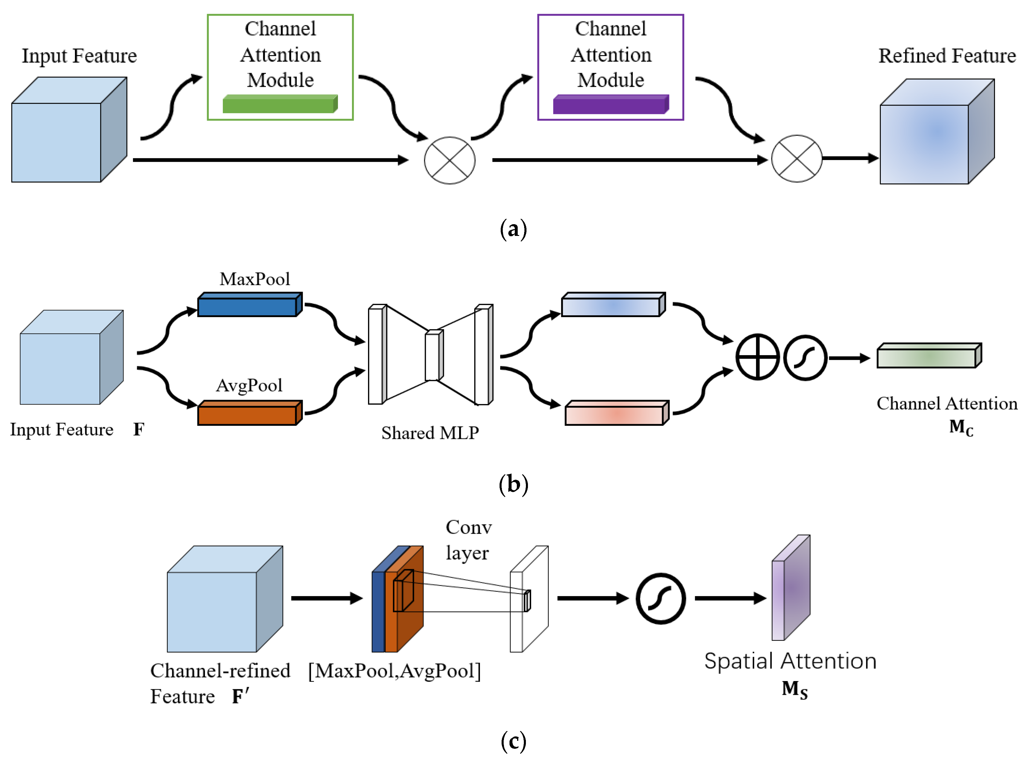
2.2. Design of CBAM-Unet Based on an Attention Mechanism
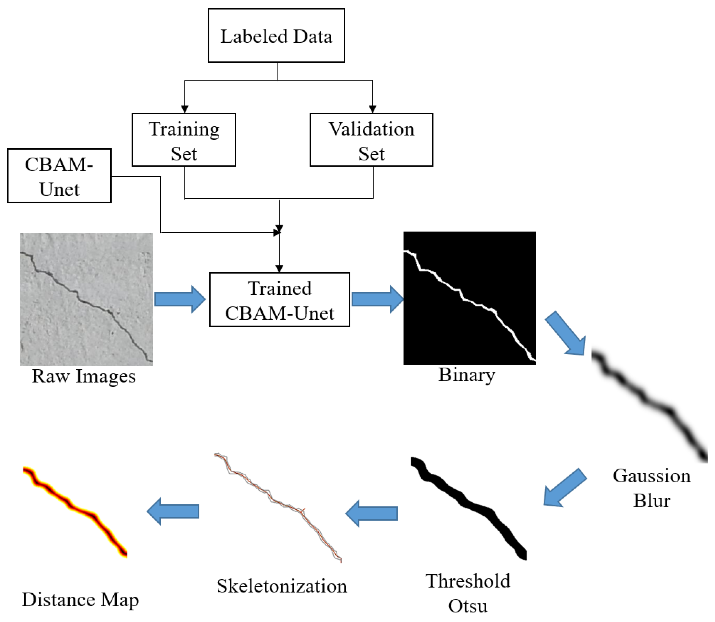
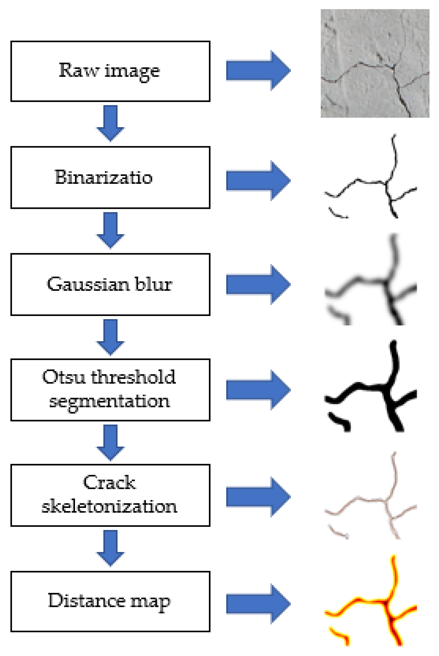
3. Crack Geometry Measurement Algorithm
- (1)
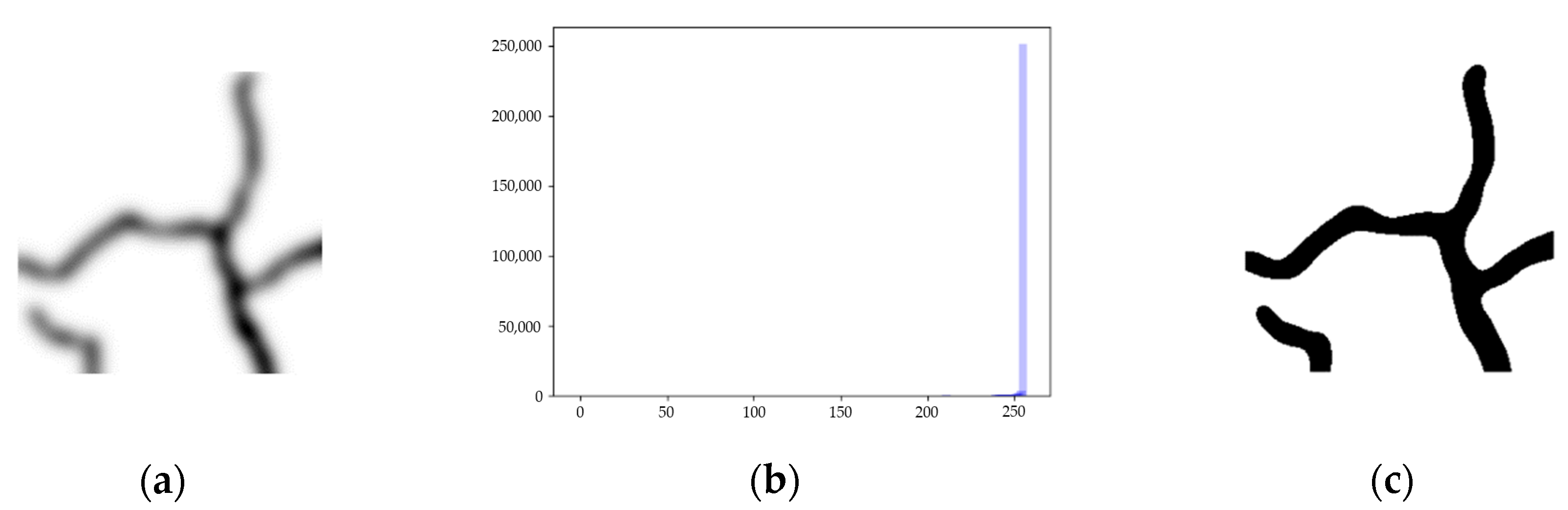
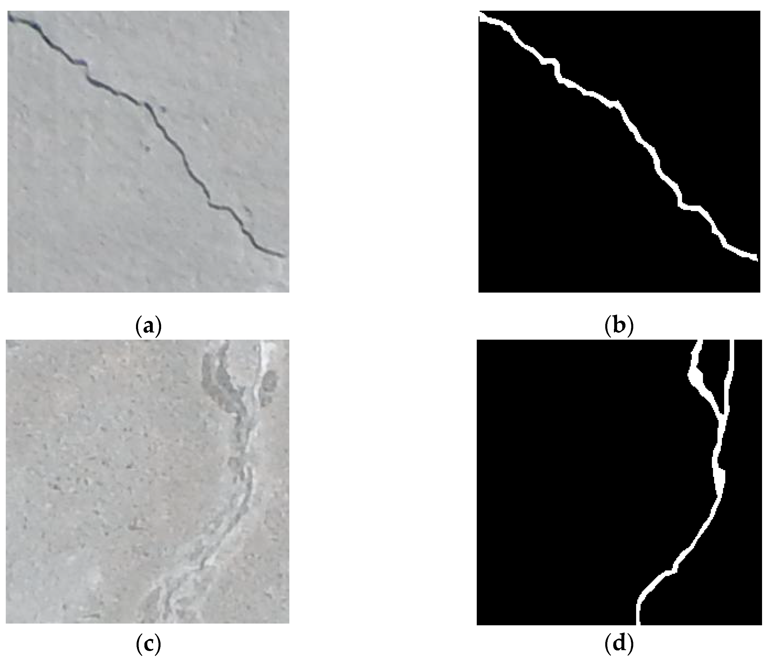
- Image binarization. The maximum inter-class variance method is used to convert each pixel of the grey-scale image to 0 or 255, reducing the number of image data and highlighting the target contours.
- (2)
- (3)
- Otsu threshold segmentation
- (4)
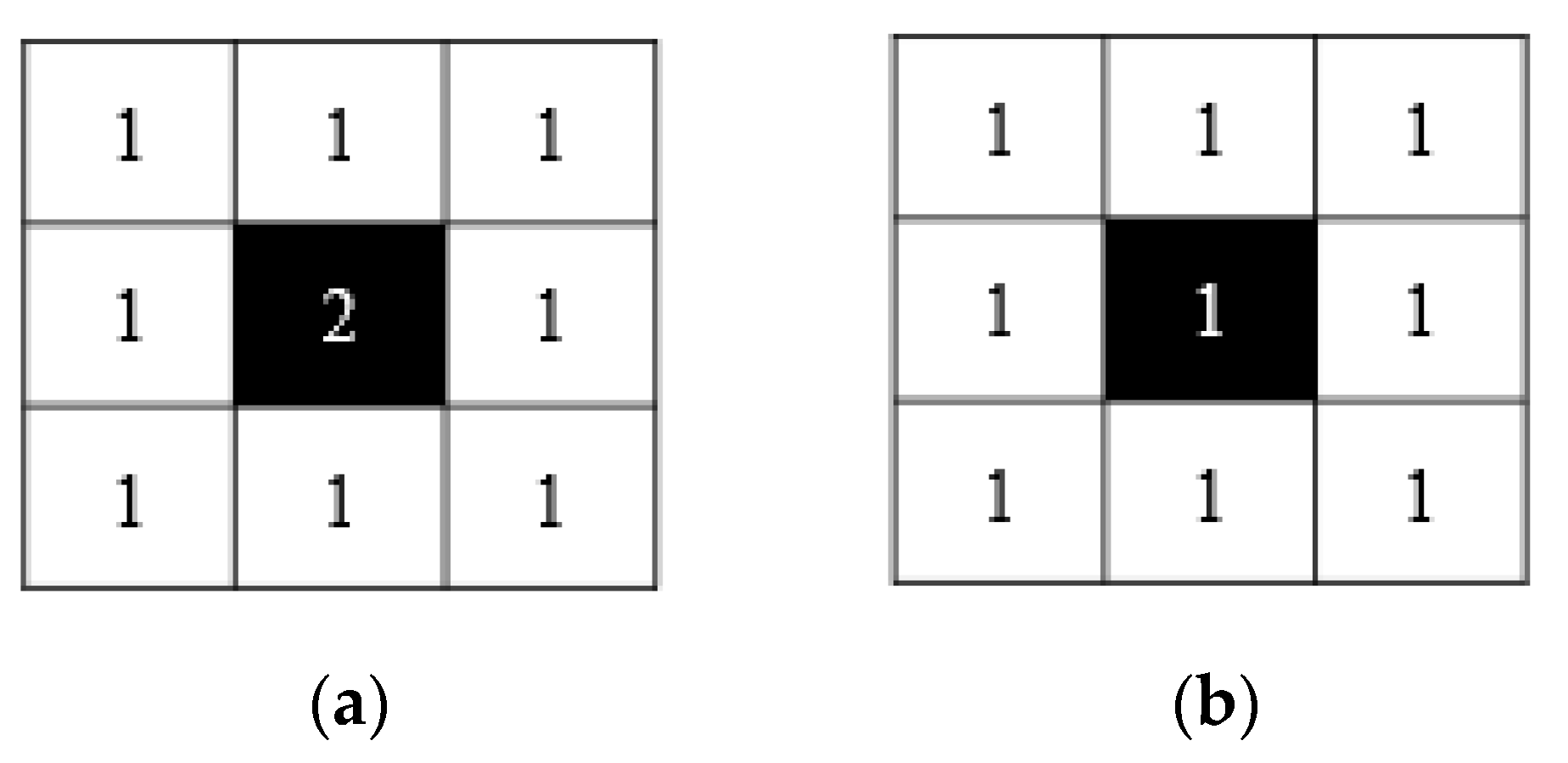
- Morphological fracture skeletonization
- (5)
- Calculation of fracture geometry parameters.
- ①
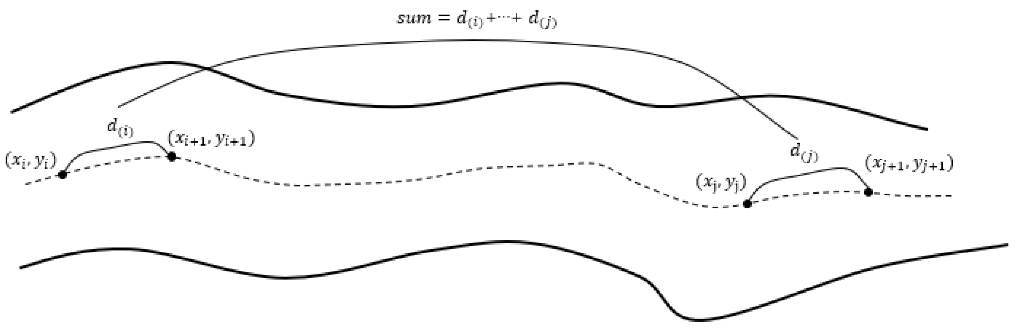
- Calculation of crack length.
- (1)
- Iterate through the debranching skeleton to obtain the coordinates of the n sets of target points between the start and end points ;
- (2)
- Calculate the straight-line distance between adjacent points. The formula is as follows.
- (3)
- Add up the straight-line distance each time:
- (4)
- Continue the above steps until the end of the calculation of the distance between the last two points.
- ②
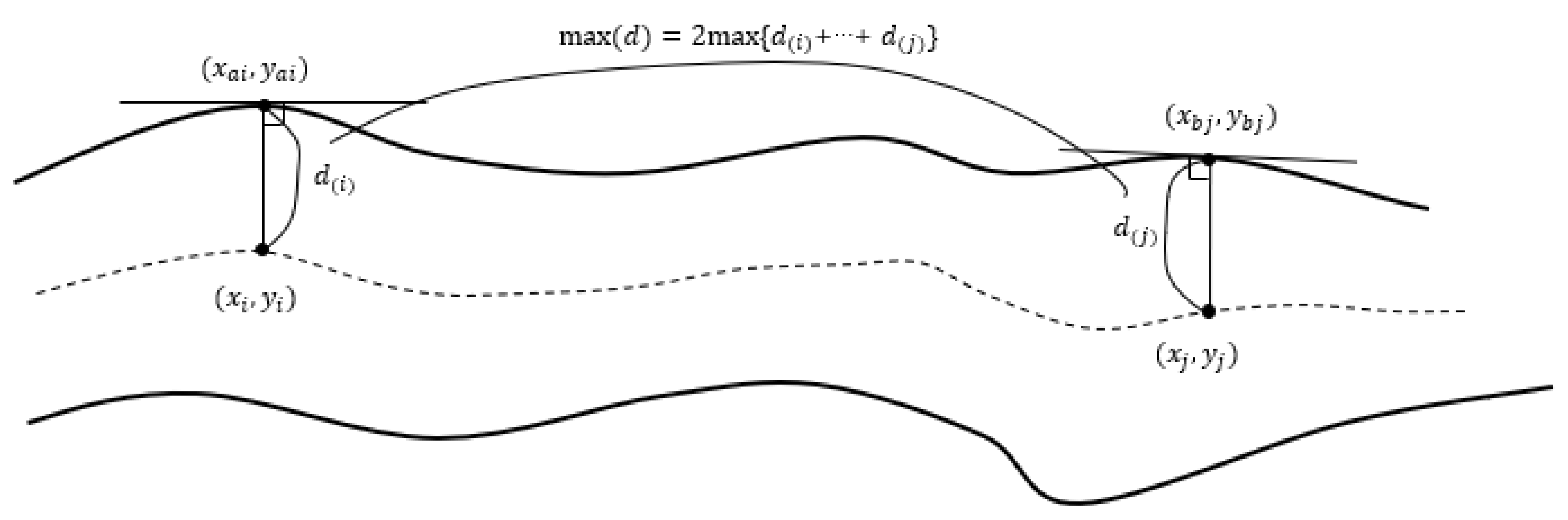
- Calculation of the maximum width of cracks.
- (1)
- Iterate through the debranching skeleton to obtain the coordinates of the n sets of target points between the start and end points .
- (2)
- From the coordinates of the points on the skeleton, the orientation of the skeleton can be obtained—i.e., its normal can be determined—and according to the method described above, the coordinates of the corresponding points on the central axis can be found. The coordinates of the target point are .
- (3)
- At this point, twice the distance between the two points is the width of the crack:
- (4)
- Compare the maximum crack width at each location:
- (5)
- Repeat until the width of the crack at the last point has been calculated.
4. Model Training
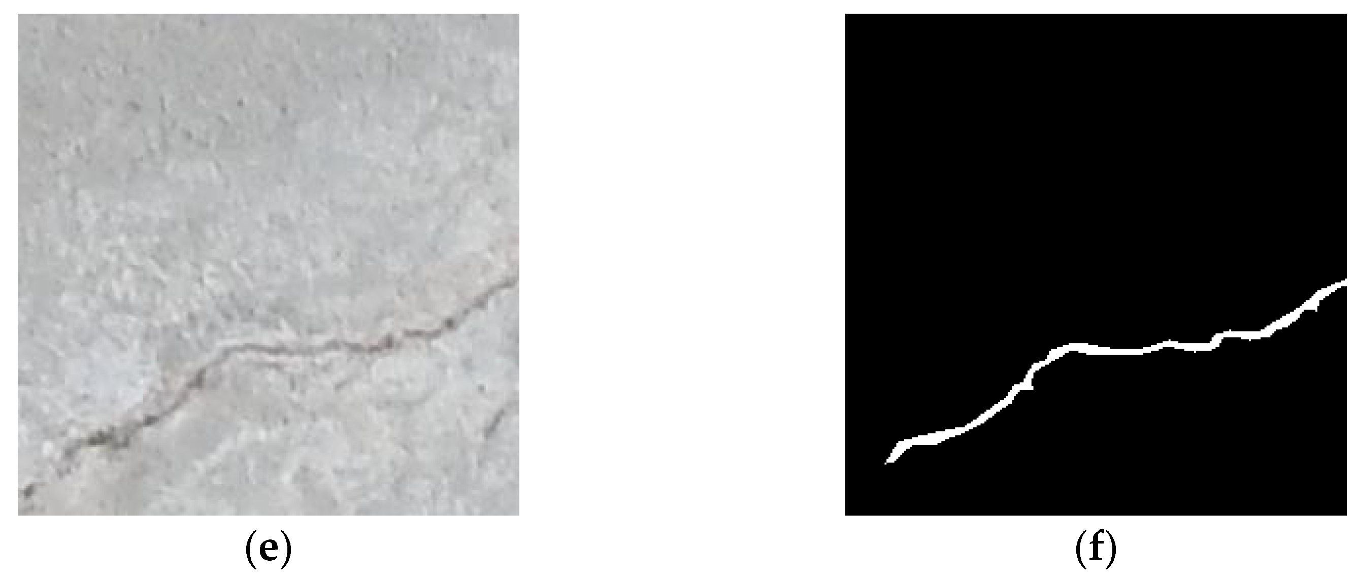
4.1. Datasets
4.2. Loss Function
4.3. Evaluation Indicators
4.4. Evaluation Indicators
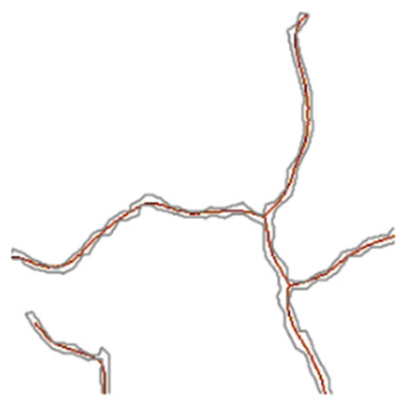
5. Verification Experiments on the Accuracy of Calculating Crack Geometry Parameters
5.1. Pixel Calibration
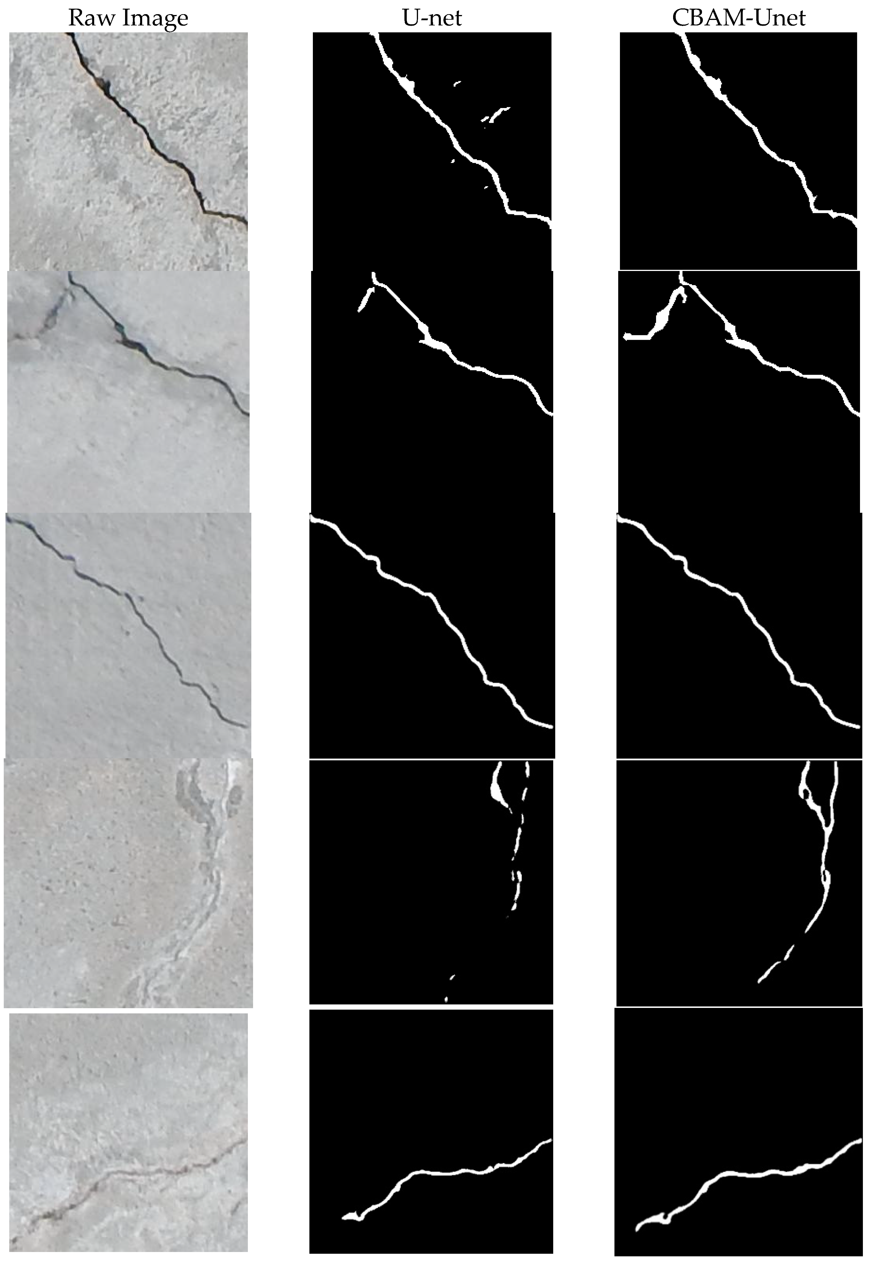
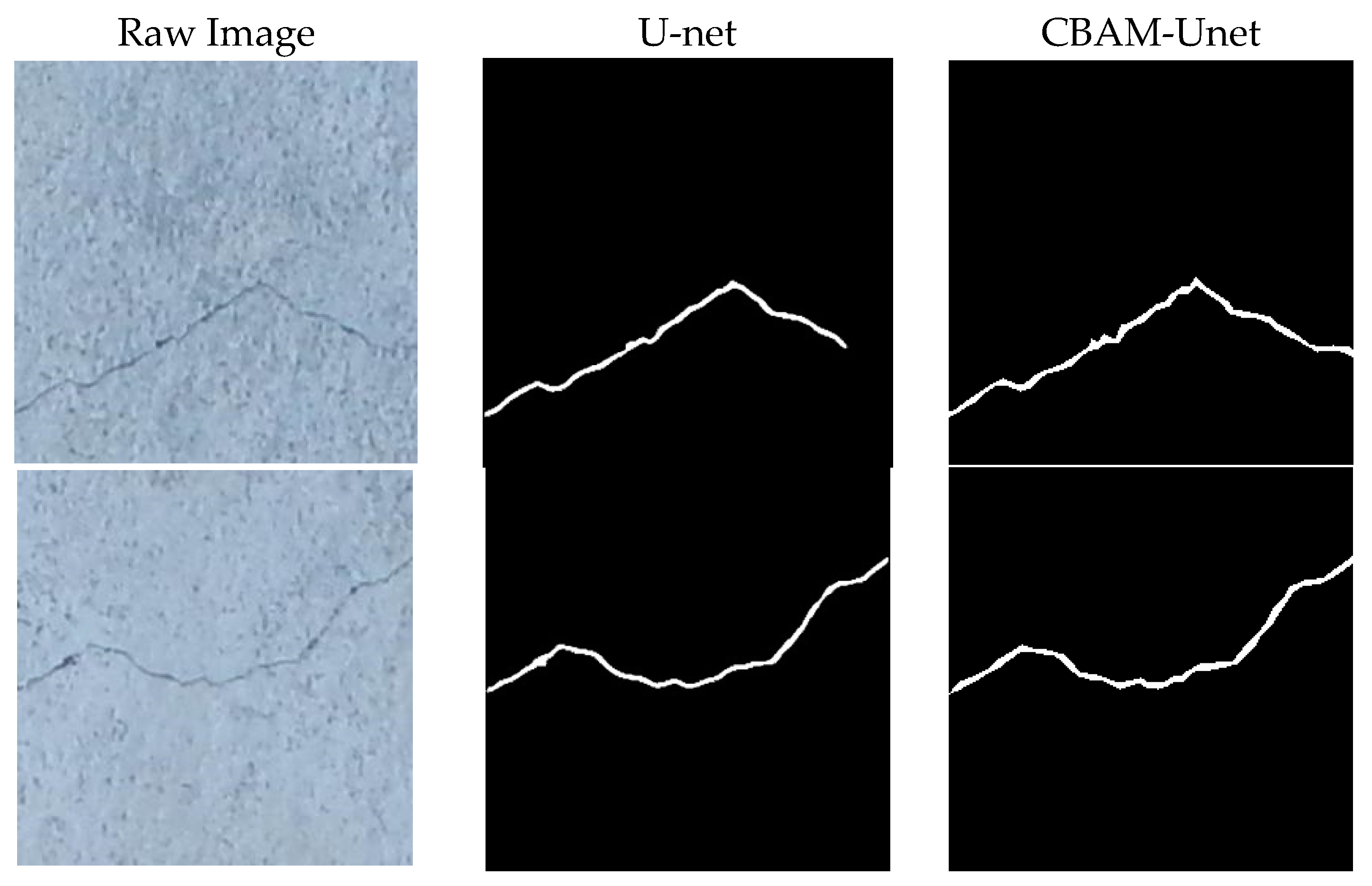
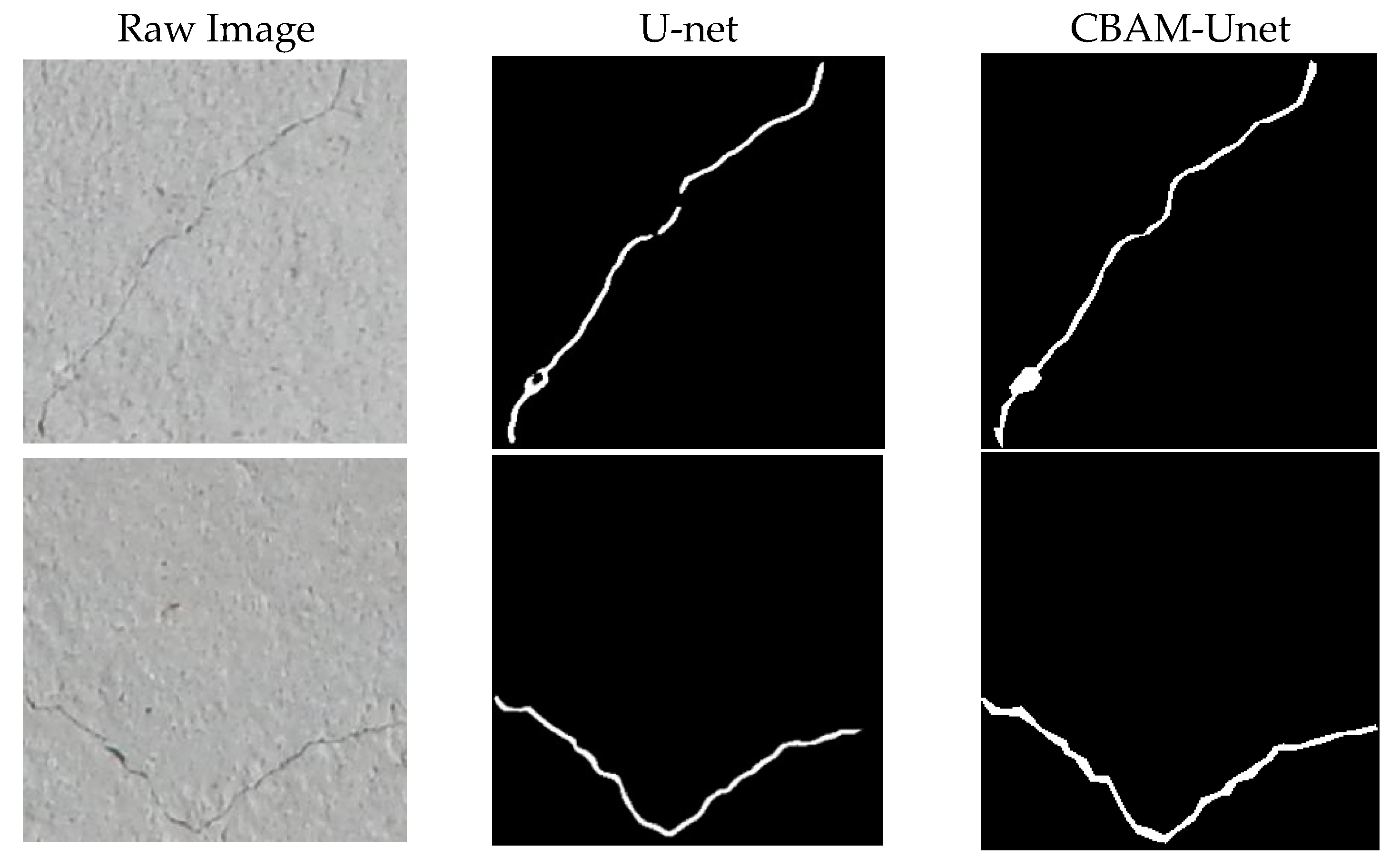
5.2. Experimental Results
6. Conclusions
Author Contributions
Funding
Data Availability Statement
Conflicts of Interest
References
- Mohan, A.; Sumathi, P. Crack Detection Using Image Processing: A Critical Review and Analysis. Alex. Eng. J. 2018, 57, 787–798. [Google Scholar] [CrossRef]
- Zhang, L.; Yang, F.; Zhang, Y.D.; Zhu, Y.J. Road crack detection using deep convolutional neural network. In Proceedings of the 2016 IEEE International Conference on Image Processing (ICIP), Phoenix, AZ, USA, 25–28 September 2016; pp. 3708–3712. [Google Scholar]
- Shi, Y.; Cui, L.; Qi, Z.; Meng, F.; Chen, Z. Automatic road crack detection using random structured forests. IEEE Trans. Intell. Transp. Syst. 2016, 17, 3434–3445. [Google Scholar] [CrossRef]
- Huang, Y.; Xu, B. Automatic inspection of pavement cracking distress. J. Electron. Imaging 2006, 15, 013017. [Google Scholar] [CrossRef]
- Zou, Q.; Cao, Y.; Li, Q.; Mao, Q.; Wan, S. CrackTree: Automatic crack detection from pavement images. Pattern Recognit. Lett. 2012, 33, 227–238. [Google Scholar] [CrossRef]
- Schmugge, S.J.; Rice, L.; Lindberg, J.; Grizziy, R.; Joffey, C.; Shin, M.C. Crack segmentation by leveraging multiple frames of varying illumination. In Proceedings of the WACV, Santa Rosa, CA, USA, 24–31 March 2017; pp. 1045–1053. [Google Scholar]
- Kaseko, M.S.; Ritchie, S.G. A neural network-based methodology for pavement crack detection and classification. Transp. Res. C Emerg. Technol. 1993, 1, 275–291. [Google Scholar] [CrossRef]
- Jahanshahi, M.R.; Masri, S.F.; Padgett, C.W.; Sukhatme, G.S. An innovative methodology for detection and quantification of cracks through incorporation of depth perception. Mach. Vis. Appl. 2013, 24, 227–241. [Google Scholar] [CrossRef]
- Teng, S.; Liu, Z.; Li, X. Improved YOLOv3-Based Bridge Surface Defect Detection by Combining High- and Low-Resolution Feature Images. Buildings 2022, 12, 1225. [Google Scholar] [CrossRef]
- Broberg, P. Surface crack detection in welds using thermography. NDT E Int. 2013, 57, 69–73. [Google Scholar]
- Yuan, Y.; Fang, J.; Lu, X.; Feng, Y. Remote Sensing Image Scene Classification Using Rearranged Local Features. IEEE Trans. Geosci. Remote Sens. 2019, 57, 1779–1792. [Google Scholar] [CrossRef]
- Wang, C.; Bai, X.; Wang, S.; Zhou, J.; Ren, P. Multiscale Visual Attention Networks for Object Detection in VHR Remote Sensing Images. IEEE Geosci. Remote Sens. Lett. 2019, 16, 310–314. [Google Scholar] [CrossRef]
- Fang, J.; Cao, X. GAN and DCN Based Multi-step Supervised Learning for Image Semantic Segmentation. In Proceedings of the Pattern Recognition and Computer Vision—First Chinese Conference, PRCV 2018, Guangzhou, China, 23–26 November 2018; Lecture Notes in Computer Science Part II. Springer: Cham, Switzerland, 2018; Volume 11257, pp. 28–40. [Google Scholar]
- Eisenbach, M.; Stricker, R.; Seichter, D.; Amende, K.; Debes, K.; Sesselmann, M.; Ebersbach, D.; Stoeckert, U.; Gross, H. How to get pavement distress detection ready for deep learning? A systematic approach. In Proceedings of the 2017 International Joint Conference on Neural Networks, IJCNN 2017, Anchorage, AK, USA, 14–19 May 2017; pp. 2039–2047. [Google Scholar]
- Xu, X.; Zhao, M.; Shi, P.; Ren, R.; He, X.; Wei, X.; Yang, H. Crack Detection and Comparison Study Based on Faster R-CNN and Mask R-CNN. Sensors 2022, 22, 1215. [Google Scholar] [CrossRef]
- Fan, Z.; Wu, Y.; Lu, J.; Li, W. Automatic Pavement Crack Detection Based on Structured Prediction with the Convolutional Neural Network. arXiv 2018, arXiv:1802.02208. [Google Scholar]
- Long, J.; Shelhamer, E.; Darrell, T. Fully Convolutional Networks for Semantic Segmentation. IEEE Trans. Pattern Anal. Mach. Intell. 2015, 39, 640–651. [Google Scholar]
- Ronneberger, O.; Fischer, P.; Brox, T. U-net: Convo1utional networks for biomedical image segmentation. In International Conference on Medical Image Computing and Computer-Assisted Intervention; Springer: Cham, Switzerland, 2015; pp. 234–241. [Google Scholar]
- Baumann, I.; Schmitt, D.; Schussler, M.; Solanki, S.K. Evolution of the large-scale magnetic field on the solar surface: A parameter study. Astron. Astrophys. 2004, 426, 1075–1091. [Google Scholar] [CrossRef]
- Liu, Z.; Cao, Y.; Wang, Y. Computer vision-based concrete crack detection using U-net fully convolutional networks. Autom. Constr. 2019, 104, 129–139. [Google Scholar] [CrossRef]
- Shankaranarayana, S.M.; Ram, K.; Mitra, K.; Sivaprakasam, M. Joint optic disc and cup segmentation using fully convolutional and adversarial networks. In Fetal, Infant and Ophthalmic Medical Image Analysis; Springer: Cham, Switzerland, 2017; pp. 168–176. [Google Scholar]
- Oktay, O.; Schlemper, J.; Folgoc, L.L.; Lee, M.; Heinrich, M.; Misawa, K.; Mori, K.; McDonagh, S.; Hammerla, N.Y.; Kainz, B.; et al. Attention u-net: Learning where to look for the pancreas. arXiv 2018, arXiv:1804.03999. [Google Scholar]
- Fan, X.; Yan, C.; Fan, J.; Wang, N. Improved U-Net Remote Sensing Classification Algorithm Fusing Attention and Multiscale Features. Remote Sens. 2022, 14, 3591. [Google Scholar] [CrossRef]
- Ma, W.; Zhou, T.; Qin, J.; Zhou, Q.; Cai, Z. Joint-attention feature fusion network and dual-adaptive NMS for object detection. Knowl.-Based Syst. 2022, 241, 108213. [Google Scholar] [CrossRef]
- Zhang, S.; Liu, Z.; Chen, Y.; Jin, Y.; Bai, G. Selective kernel convolution deep residual network based on channel-spatial attention mechanism and feature fusion for mechanical fault diagnosis. ISA Trans. 2022; in press. [Google Scholar] [CrossRef]
- Li, A.; Qi, J.; Lu, H. Multi-attention guided feature fusion network for salient object detection. Neurocomputing 2020, 411, 416–427. [Google Scholar] [CrossRef]
- Fu, J.; Liu, J.; Tian, H.; Li, Y.; Bao, Y.; Fang, Z.; Lu, H. Dual Attention Network for Scene Segmentation. In Proceedings of the 2019 IEEE/CVF Conference on Computer Vision and Pattern Recognition (CVPR), Long Beach, CA, USA, 15–20 June 2019. [Google Scholar]
- Shen, Y.; Wen, Y. Convolutional Neural Network optimization via Channel Reassessment Attention module. Digit. Signal Process. 2020, 123, 103408. [Google Scholar] [CrossRef]
- Zhuo, Q.; Yang, T.; Zhang, J. Research on classification algorithms for attention mechanism. In Proceedings of the 2020 19th International Symposium on Distributed Computing and Applications for Business Engineering and Science (DCABES), Xuzhou, China, 16–19 October 2020. [Google Scholar]
- Cui, J.; Wang, D.; Liu, J. Single image defogging algorithm based on Gaussian blur. Autom. Instrum. 2021, 1, 9–11, 16. [Google Scholar] [CrossRef]
- Chen, Q. Modified two-dimensional Otsu image segmentation algorithm and fast realisation. IET Image Process. 2012, 6, 426–433. [Google Scholar] [CrossRef]
- Xu, X.; Xu, S.; Jin, L.; Song, E. Characteristic analysis of Otsu threshold and its applications. Pattern Recognit. Lett. 2021, 32, 956–961. [Google Scholar] [CrossRef]
- Alsaeed, D.; Bouridane, A.; El-Zaart, A. A novel fast Otsu digital image segmentation method. Int. Arab. J. Inf. Technol. 2016, 13, 427–434. [Google Scholar]
- Dorafshan, S.; Maguire, M.; Thomas, R. SDNET2018: A Concrete Crack Image Dataset for Machine Learning Applications; Utah State University: Logan, UT, USA, 2018. [Google Scholar]


| Environment | Configuration |
|---|---|
| Operating system | Windows10 |
| CPU | Intel i5 12400F @ 2.5 GHz |
| GPU | Nvidia GeForce RTX3060 |
| RAM | 16 G |
| Memory | 500 G |
| Programming language | Python3.8 |
| Deep learning framework | Pytorch |
| Evaluation Index | Computational Formula |
|---|---|
| PA | |
| CPA | |
| Recall | |
| IoU |
| Methods | PA | CPA | Recall | IoU |
|---|---|---|---|---|
| U-net | 87.32% | 84.96% | 96.26% | 82.16% |
| CBAM-Unet | 92.66% | 92.20% | 97.13% | 89.53% |
| Number | Crack Width (mm) | Inaccuracy | ||
|---|---|---|---|---|
| Calculated Values (mm) | Measured Values (mm) | Absolute Values/mm | Relative Values/% | |
| 1 | 0.612 | 0.630 | −0.018 | 2.9 |
| 2 | 0.962 | 0.980 | −0.018 | 1.8 |
| 3 | 1.448 | 1.360 | 0.088 | 6.5 |
| 4 | 1.560 | 1.620 | −0.060 | 3.7 |
| 5 | 1.208 | 1.260 | −0.052 | 4.1 |
| 6 | 0.826 | 0.840 | −0.014 | 1.7 |
| 7 | 2.244 | 2.200 | 0.044 | 2.0 |
| 8 | 1.762 | 1.720 | 0.042 | 2.4 |
| 9 | 1.706 | 1.620 | 0.086 | 5.3 |
| 10 | 2.248 | 2.160 | 0.088 | 4.1 |
| Number | Crack Length (mm) | Inaccuracy | ||
|---|---|---|---|---|
| Calculated Values (mm) | Measured Values (mm) | Absolute Values/mm | Relative Values/% | |
| 1 | 39.308 | 39.940 | −0.632 | 1.58 |
| 2 | 36.600 | 38.368 | −1.768 | 4.61 |
| 3 | 38.256 | 39.572 | −1.316 | 3.33 |
| 4 | 36.272 | 38.224 | −1.952 | 5.11 |
| 5 | 38.400 | 39.658 | −1.258 | 3.17 |
| 6 | 32.068 | 34.720 | −2.652 | 7.64 |
| 7 | 34.496 | 35.970 | −1.474 | 4.10 |
| 8 | 37.568 | 35.980 | 1.588 | 4.41 |
| 9 | 34.884 | 36.234 | −1.350 | 3.73 |
| 10 | 36.544 | 37.896 | −1.352 | 3.57 |
Publisher’s Note: MDPI stays neutral with regard to jurisdictional claims in published maps and institutional affiliations. |
© 2022 by the authors. Licensee MDPI, Basel, Switzerland. This article is an open access article distributed under the terms and conditions of the Creative Commons Attribution (CC BY) license (https://creativecommons.org/licenses/by/4.0/).
Share and Cite
Su, H.; Wang, X.; Han, T.; Wang, Z.; Zhao, Z.; Zhang, P. Research on a U-Net Bridge Crack Identification and Feature-Calculation Methods Based on a CBAM Attention Mechanism. Buildings 2022, 12, 1561. https://doi.org/10.3390/buildings12101561
Su H, Wang X, Han T, Wang Z, Zhao Z, Zhang P. Research on a U-Net Bridge Crack Identification and Feature-Calculation Methods Based on a CBAM Attention Mechanism. Buildings. 2022; 12(10):1561. https://doi.org/10.3390/buildings12101561
Chicago/Turabian StyleSu, Huifeng, Xiang Wang, Tao Han, Ziyi Wang, Zhongxiao Zhao, and Pengfei Zhang. 2022. "Research on a U-Net Bridge Crack Identification and Feature-Calculation Methods Based on a CBAM Attention Mechanism" Buildings 12, no. 10: 1561. https://doi.org/10.3390/buildings12101561