An Innovative Structural Dynamic Identification Procedure Combining Time Domain OMA Technique and GA

Abstract

In this paper an innovative and simple Operational Modal Analysis (OMA) method for structural dynamic identification is proposed. It combines the recently introduced Time Domain–Analytical Signal Method (TD–ASM) with the Genetic Algorithm (GA). Specifically, TD–ASM is firstly employed to estimate a subspace of candidate modal parameters, and then the GA is used to identify the structural parameters minimizing the fitness value returned by an appropriately introduced objective function. Notably, this method can be used to estimate structural parameters even for high damping ratios, and it also allows one to identify the Power Spectral Density (PSD) of the structural excitation. The reliability of the proposed method is proved through several numerical applications on two different Multi Degree of Freedom (MDoF) systems, also considering comparisons with other OMA methods. The results obtained in terms of modal parameters identification, Frequency Response Functions (FRFs) matrix estimation, and structural response prediction show the reliability of the proposed procedure.

1. Introduction

1.1. Preliminaries and Problem Statement

The identification of the dynamic properties of a system, i.e., its natural frequencies, damping ratios, and modal shapes, is nowadays common in many branches of engineering and has been used for different purposes both in mechanical and in civil and aerospace engineering applications [1]. It can be performed by using traditional Experimental Modal Analysis (EMA) methods or Operational Modal Analysis (OMA) methods. EMA methods require the knowledge of both structural excitation (input) and structural response (output), while OMA methods allow one to identify the dynamic properties of a system, assumed as linear and time-invariant [2], without knowledge of the structural excitation [3] that is due to ambient vibrations and usually modelled as a stationary [4] white noise [5]. OMA methods can be employed for different purposes such as model validation [6], calibration of Finite Elements Models (FEMs) [7], vibration control [8,9], Structural Health Monitoring (SHM) [10,11,12,13,14], damage detection [15], and structural identification [16,17,18]. Applications of OMA were conducted on bridges [19,20,21], historical buildings [17,22], dams [23], tall buildings [24,25], offshore platforms [26,27], and other kinds of structure [28,29,30].

In structural engineering, the identification of the dynamic properties is the first step required to perform an SHM; indeed, if there are damages to the structural elements due to degradation of the materials or strong external excitations, then the dynamic behavior of the structure changes along with its dynamic properties, and therefore to identify structural damages, it is necessary to use identification methods capable of estimating the dynamic properties with high precision. However, the precision of OMA methods usually decreases when the damping ratio increases and/or there are closely spaced frequencies. Moreover, they do not return information regarding the structural input.

The aim of this paper is to propose a simple-to-use identification method that allows the modal parameters to be estimated, also in the case of high damping ratios, and that can provide information on the structural input.

1.2. State of the Art

In the literature, there are many OMA methods for structural identification that can be classified according to the domain in which they are developed.

Peak Picking (PP) [31] is a simple frequency domain procedure to estimate the natural frequencies from the peaks of the Power Spectral Densities (PSDs) and, if linked to the Half Power Bandwidth Method (HP) [31], allows the damping ratios to be identified. Although PP is attractive for its simplicity, it can be used only for systems that have low values of damping ratios and well-separated modes.

Frequency Domain Decomposition (FDD) was introduced in 2000 [32,33], and soon it became one of the most popular OMA methods in the frequency domain. Frequencies and modal shapes are estimated by performing a Singular Value Decomposition (SVD) [5] of the PSD matrix. Although FDD is fast and simple to use, it cannot identify the damping ratios. For this reason, a new version of FDD, called Enhanced Frequency Domain Decomposition (EFDD), was developed [34]. EFDD has higher accuracy than FDD, but the estimation of the damping ratios is still an open issue [1].

The Natural Excitation Technique (NExT) [35] is a time domain OMA method that exploits the auto- and cross-correlation functions of the response process. It has a deterministic framework [1], but its combination with algorithms such as Eigensystem Realization Algorithm (ERA) [36], PolyReference Complex Exponential (PRCE) [37], or Extended Ibrahim Time Domain (EITD) [38] can be classified as an OMA method to identify the dynamic properties, also in the case of closely spaced modes [1].

Auto Regressive Moving Average (ARMA) [39], or Auto Regressive Moving Average Vector (ARMAV) in case of multiple excitations [40], is based on the prediction of the current value of a time series considering the past values and the prediction error. It is usually linked to another method, such as the Prediction Error Method (PEM) [41], the Liner Multi-Stage (LMS) method [42], or the Instrument Variable Method (IVM) [42]. Since the MA part causes non-linearity, the identification process must be iteratively implemented, and thus it is computationally intensive.

Time Domain Decomposition (TDD) [43] is based on a Single Degree of Freedom (SDoF) approach; in fact, for Multi Degree of Freedom (MDoF) systems, it is necessary to filter the signal to obtain mono-component signals [43]. From the correlation functions matrix of the filtered signals, it is possible to estimate the modal shapes by performing an SVD [43]. Frequencies and damping ratios can be estimated from the mono-component signals by using PP and HP. Since it is based on an SDOF approach, it is difficult to identify the dynamic properties in the case of closely spaced modes [1].

The most used time domain OMA method is Stochastic Subspace Identification (SSI) [1], first developed in 1991 [44]. There are two main SSI algorithms [45]: SSI covariance driven (SSI-COV), and SSI data driven (SSI-DATA). Both of them can be implemented with the Principle Component (PC) method, the Unweighted Principle Component (UPC) method, or the Canonical Variant Analysis (CVA) method. SSI-COV [46] exploits the output covariance matrix, called the Toeplitz matrix, that is decomposed in two different ways, namely, into the product of an observability matrix and a controllability matrix and by using an SVD. With this information, it is possible to estimate the state transition matrix and, by performing an eigenvalue decomposition, it is possible to estimate the modal properties of the system. SSI-DATA [47], developed in 1993, uses a QR decomposition of the data Hankel matrix in order to project the future output in the past output, and then an SVD of the projection matrix is performed to identify the dynamic properties. PC, UPC, or CVA are used to weigh the matrices before applying the SVD [1,3,5]. SSI is a stable and precise method, but, in general, it is very difficult to mathematically implement [1].

The Analytical Signal Method (ASM) is a recently introduced hybrid method [17] that uses the mono-component correlation functions obtained from the Inverse Fourier Transform (IFT) of the filtered PSDs. Since the Analytical Signal (AS) is very sensible to the minimum change of the natural frequencies [48,49,50], it is used in ASM to better identify them. Precisely, the AS of the mono-component correlation functions is decomposed in envelope and phase, from which it is possible to estimate the damping ratios and the natural frequencies. ASM is a fast OMA method, but it cannot identify the modal shapes.

The Time Domain–Analytical Signal Method (TD–ASM) is a recent OMA method very similar to ASM but entirely developed in the time domain [18]. In TD–ASM, firstly the correlation functions matrix of the structural response is decomposed into mono-component correlation functions by using an SVD, and then the natural frequencies and the damping ratios can be estimated from the AS of the mono-component correlation functions [18]. For systems that have equal masses, the modal shapes can be estimated by performing an SVD of the correlation functions matrix, but if the structural system has different masses, TD–ASM cannot identify the modal shapes except the dominant one. However, also in the cases of different masses, the frequencies and the damping ratios can be identified with sufficient accuracy, and the discrepancy between the estimated dominant modal shape and the exact one is very low and less than that reported by other OMA methods [18].

OMA identification methods can also be linked with Artificial Intelligence (AI) or with Evolutionary Algorithms (EAs).

Procedures that link OMA with AI can be used to detect and/or localize damages [51,52,53,54]. They usually follow a Machine Learning (ML) approach [51] that consists of training an Artificial Neural Network (ANN) through the use of different samples composed by an input (that can be the structural response or its statistical properties) and an output (that is the presence or not of the damage and/or its localization). The training can be supervised or unsupervised [55], but for damage detection, the supervised training is generally used [51]. However, for novel real structures, it is impossible to have real data on the damaged case, and thus in order to overcome this limit, two different procedures can be followed [51]. The first one is to use the data obtained from FEM (appropriately calibrated) and the data obtained from in situ investigations for the undamaged structure, while for the damaged structure, only the data obtained from an FEM can be used. The second way is to use unsupervised ML or unsupervised Deep Learning (DL) approaches, but very few studies have been conducted in this regard [51]. However, this kind of approach does not allow one to have full control of each single step performed by the AI, and the simulation of several input–output samples deriving from FEM can require a very high computational burden.

Procedures that use EA, such as the Genetic Algorithm (GA) or Particle Swarm Optimization (PSO), usually minimize or maximize the fitness value obtained from an objective function called fitness function [56,57]. The latter is properly designed depending on the purpose to be achieved. Nowadays, these kinds of techniques are used, for instance, to detect damages [58] or to calibrate FEM [59].

1.3. Highlights of the Proposed Method

In this paper, an innovative semi-automatic OMA method for structural dynamic identification called the Time Domain–Analytical Signal Method with Genetic Algorithm (TAGA) is proposed. It exploits the advantages of TD–ASM, i.e., accurate identification of the dominant modal shape and an initial identification of natural frequencies and damping ratios; furthermore, thanks to a linking with the GA, the modal shapes can be identified also in the case of systems that have different masses. In the proposed method, an appropriate fitness function is introduced to reduce the discrepancies between the PSDs of the recorded signals and the PSDs estimated through the use of the GA. The estimated PSDs are calculated by varying the values of the modal parameters with the limits imposed by a subspace appropriately chosen considering the frequencies and the damping ratios previously estimated with the use of TD–ASM. TAGA is simple to use, leads to good results also in the case of high values of the damping ratios and, unlike other OMA methods, allows one to identify the PSD of the structural input.

2. Proposed Method and Numerical Validation

2.1. Proposed Method

The proposed method is articulated in two different parts: first, TD–ASM is applied, and then GA optimization is performed. For the sake of clarity, in this subsection, all the steps of each part are described in detail.

2.1.1. Time Domain–Analytical Signal Method (TD–ASM)

TD–ASM is a recently introduced time domain OMA method that can be considered as a modified version of the ASM [18]. For SDoF systems, ASM estimates the natural frequency and the damping ratio, respectively, from the phase and the envelope of the AS of the response’s correlation functions. The latter is obtained by performing the IFT of the response’s PSD [17] calculated, for instance, by using the Welch method [60,61]. TD–ASM does not require the calculation of the PSD, since it directly calculates the correlation function of the response process. Then it estimates the natural frequency and the damping ratio from the phase and the envelope of the AS of the response’s correlation functions. For MDoF systems, the procedure is the same, but a decomposition of the correlation functions matrix is required before proceeding as in the SDoF case. For an MDoF system TD–ASM can be conducted using the following steps [18]:

• Acquisition of the structural response process;
• Estimation of the response process’ correlation functions matrix;
• Singular Value Decomposition (SVD) of the correlation functions matrix in zero;
• Estimation of the mono-component correlation functions;
• Reconstruction of the Analytical Signal (AS) of each mono-component auto-correlation function;
• Estimation of frequencies and damping ratios.

The equation of motion of an MDoF system with mass matrix $M$, stiffness matrix $K$, and damping matrix $C$, excited by a ground acceleration $W\left(t\right)$ assumed as a white noise process, is

$$M\ddot{X}\left(t\right)+C\dot{X}\left(t\right)+KX\left(t\right)=-MW\left(t\right)$$

(1)

where $X\left(t\right)$, $\dot{X}\left(t\right)$, and $\ddot{X}\left(t\right)$ are the response processes, respectively, in terms of displacement, velocity, and acceleration. The correlation function matrix of the response process $X\left(t\right)$, labeled as $R_X\left(\tau \right)$, can be computed taking into account that

$$R_{X_i{X}_j}\left(\tau \right)=E\left[X_i\left(t\right)X_j\left(t+\tau \right)\right]$$

(2)

in which $E[·]$ is the stochastic mean operator, $i=1,2,\dots ,n_{dof}$, $j=1,2,\dots ,n_{dof}$, and $n_{dof}$ is the number of the system’s degrees of freedom. After the computation of the correlation functions matrix, an SVD of the latter in $\tau =0$ can be performed, and thus $R_X\left(0\right)$, that is, the covariance matrix of the response process, can be decomposed in the form

$$R_X\left(0\right)=US{V}^H$$

(3)

where $S$ is a diagonal matrix that contains the singular values of $R_X\left(0\right)$, $U$ and $V$ are, respectively, the left and the right eigenvectors of $R_X\left(0\right)$, and the apex H denotes the conjugate transpose. Note that since $R_X\left(0\right)$ is a normal matrix, i.e., it is square and the relation $R_X^T\left(0\right)R_X\left(0\right)=R_X\left(0\right)R_X^T\left(0\right)$ is valid, $U=V$. Further, since $R_X\left(0\right)$ is a real matrix, the conjugate transpose and the transpose are the same matrix, and thus Equation (3) becomes [18]

$$R_X\left(0\right)=US{U}^T.$$

(4)

As it can be seen, Equation (4) has a form that is similar to the modal decomposition of the correlation functions matrix for classically damped systems, i.e., [5,62]:

$$R_X\left(\tau \right)=\tilde{\mathsf{\Phi }}{R}_{\tilde{Y}}\left(\tau \right){\tilde{\mathsf{\Phi }}}^T$$

(5)

where $R_{\tilde{Y}}\left(\tau \right)$ is the correlation functions matrix in modal space, $\tilde{Y}\left(t\right)$ is the structural response in modal space, and $\tilde{\mathsf{\Phi }}$ is the modal matrix. It is emphasized that the modal matrix represents the structural system’s modal shapes $\mathsf{\Phi }$ normalized with respect to the mass matrix. For systems having equal masses, the smaller the damping and the more $U\to \mathsf{\Phi }$ [18], and thus the modal shapes can be directly estimated from the SVD of the correlation functions matrix. Since $U{U}^{-1}=U^{-1}U=I$, then the mono-component correlation functions can be calculated as the terms present in the diagonal of $R_Y\left(\tau \right)$ [18], the latter being defined as

$$R_Y\left(\tau \right)=U^{-1}{R}_X\left(\tau \right)U^{-T}$$

(6)

In order to estimate the mono-component correlation functions also for systems that have different masses, Equation (6) can be applied, but in this case, TD–ASM cannot identify the modal shapes except the dominant one.

Each mono-component correlation function in the diagonal of $R_Y\left(\tau \right)$, denoted as $R_{Y_j}\left(\tau \right)$, can be used to reconstruct its AS. This is a complex signal [48,49,50] whose real part is the correlation function itself, and the imaginary part is its Hilbert transform. Thus, the AS of the j-th mono-component correlation function is given as [18]

$$Z_{Y_j}\left(\tau \right)=R_{Y_j}\left(\tau \right)+i{\widehat{R}}_{Y_j}\left(\tau \right)$$

(7)

in which ${\widehat{R}}_{Y_j}\left(\tau \right)$ is the Hilbert transform of the j-th mono-component correlation function $R_{Y_j}\left(\tau \right)$. The Hilbert transform of $R_{Y_j}\left(\tau \right)$ represents the convolution between $R_{Y_j}\left(\tau \right)$ and $1/\left(\pi \tau \right)$. It is calculated as [18]

$${\widehat{R}}_{Y_j}\left(\tau \right)=\frac{1}{\pi }\wp {\displaystyle \underset{-\infty }{\overset{\infty }{\int }}\frac{R_{Y_j}\left(\tilde{\tau }\right)}{\tau -\tilde{\tau }}d\tilde{\tau }}$$

(8)

where $\wp$ is the principal value. The AS in Equation (7) can be expressed in polar form as [18]

$$Z_{Y_j}\left(\tau \right)=A_j\left(\tau \right)e^{i{\vartheta }_j\left(\tau \right)}$$

(9)

where $A_j\left(\tau \right)$ and ${\vartheta }_j\left(\tau \right)$ are, respectively, the envelope and the phase of the AS, and they are calculated as [18]

$$A_j\left(\tau \right)=\sqrt{R_{Y_j}{\left(\tau \right)}^2+{\widehat{R}}_{Y_j}{\left(\tau \right)}^2}\approx {\sigma }_{Y_j}^2{e}^{-2\pi f_j{\zeta }_j\tau }$$

(10)

$${\vartheta }_j\left(\tau \right)=\arctan \left[\frac{{\widehat{R}}_{Y_j}\left(\tau \right)}{R_{Y_j}\left(\tau \right)}\right]\approx 2\pi f_j\sqrt{1-{\zeta }_j^2}\tau$$

(11)

in which ${\sigma }_{Y_j}^2$ is the variance of the j-th mono-component response process $Y_j\left(t\right)$. By performing the first derivative of the phase ${\vartheta }_j\left(\tau \right)$ and dividing by $2\pi$, it is possible to obtain the instantaneous damped frequency ${\overline{f}}_j\left(\tau \right)$, i.e., [17,18]

$${\overline{f}}_j\left(\tau \right)=\frac{1}{2\pi }\frac{d}{d\tau }\left[{\vartheta }_j\left(\tau \right)\right],$$

(12)

and thus the j-th damped frequency of the structural system $f_j\sqrt{1-{\zeta }_j^2}$ can be estimated performing the mean of the instantaneous damped frequency in Equation (12). The damping ratio can be calculated from the envelope; in fact, by performing the logarithm of Equation (10) it is possible to obtain the linear form [17,18]

$$\ln \left[A_j\left(\tau \right)\right]=\ln \left[{\sigma }_{Y_j}^2\right]-2\pi f_j{\zeta }_j\tau =c_{2,j}+c_{1,j}\tau ,$$

(13)

and thus the j-th damping ratio of the structural system can be estimated as [17,18]

$${\zeta }_j=-\frac{c_{1,j}}{2\pi f_j}=\sqrt{\frac{{\overline{c}}_{1,j}^2}{1+{\overline{c}}_{1,j}^2}}$$

(14)

in which ${\overline{c}}_{1,j}=c_{1,j}/\left(2\pi f_j\sqrt{1-{\zeta }_j^2}\right)$. After the estimation of the j-th damped frequency $f_j\sqrt{1-{\zeta }_j^2}$ and the j-th damping ratio ${\zeta }_j$, the j-th natural frequency $f_j$ can be easily calculated.

TD–ASM is a very user-friendly method that can be used also by users that have little to no knowledge in signal analysis and stochastic dynamics [18]. However, TD–ASM cannot identify all the modal shapes of systems that have different masses. To overcome this limit, the proposed method links it with the GA. In the next sub-subsection there is a detailed description of how the information obtained by using TD–ASM can be exploited to model an optimization problem and how to solve it by using the GA.

2.1.2. Genetic Algorithm (GA)

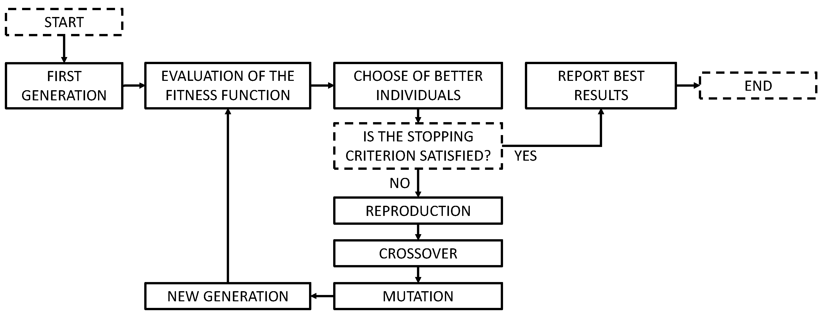
The GA, often used in optimization problems, is one of the EAs [56]. It is based on Darwin’s natural selection according to which, with the increase of generations, there is an increase of individuals presenting optimal characteristics for the environment in which they live [56]. From an optimization point of view, the GA finds the parameters that minimize or maximize a fitness value dependent on a certain function called fitness function. To perform a GA optimization, it is necessary to choose not only the fitness function but also the domain of the parameters to be identified, the number of individuals of the initial population, and the stopping criterion. The latter is the condition to be satisfied for the stoppage of the evolutionary procedure to occur, and it is usually selected among maximum number of generations, maximum time for the optimization procedure, maximum number of stall generations, or achievement of a certain fitness value. The GA begins with the creation of the first generation made up of a preselected number of individuals randomly chosen among all possible combinations and, for each of them, the fitness value is calculated. Individuals with the best fitness values are selected to create a new generation of individuals obtained through reproduction, crossover, and mutation operations [57]. This evolutionary procedure will continue until the stopping criterion is satisfied. The classical GA scheme is depicted in Figure 1.

For the proposed method, the domain of the parameters to be identified as

$$f_j\in \left[f_j^{\left(est\right)}-{\epsilon }_f{f}_j^{\left(est\right)};f_j^{\left(est\right)}+{\epsilon }_f{f}_j^{\left(est\right)}\right]$$

(15)

$${\zeta }_j\in \left[{\zeta }_j^{\left(est\right)}-{\epsilon }_{\zeta }{\zeta }_j^{\left(est\right)};{\zeta }_j^{\left(est\right)}+{\epsilon }_{\zeta }{\zeta }_j^{\left(est\right)}\right]$$

(16)

$${\varphi }_{ik}\in \left[-1;1\right]k=2,\dots ,n_{dof}$$

(17)

and

$$S_0\in \left[0;S_{0,\max }\right],$$

(18)

respectively, for the frequencies, the damping ratios, the modal shapes, and the constant value of the PSD of the white noise $W\left(t\right)$. The apex $\left(est\right)$ indicates that the frequencies and the damping ratios are estimated through the use of TD–ASM, $f_j^{\left(est\right)}\pm {\epsilon }_f{f}_j^{\left(est\right)}$ and ${\zeta }_j^{\left(est\right)}\pm {\epsilon }_{\zeta }{\zeta }_j^{\left(est\right)}$ represent the range of variations of the estimated frequencies and damping ratios, and $S_{0,\max }$ is the maximum constant value of the white noise’s PSD. The values of ${\epsilon }_f$ and ${\epsilon }_{\zeta }$ have to be chosen by taking into account the precision of TD–ASM. Particularly, since TD–ASM leads to good results in terms of frequencies identification, a small value of ${\epsilon }_f$ (5–10%) can be chosen. For ${\epsilon }_{\zeta }$, a greater value (40–50%) may be needed because the precision of TD–ASM in terms of damping identification can decrease for modes that give less contribution to the total motion. Obviously, if ${\epsilon }_f$ and ${\epsilon }_{\zeta }$ increase, then the required computational burden increases, since a larger domain must be explored. It should be noted that in Equation (17), $k=2,\dots ,n_{dof}$ because the first modal shape (estimated through the use of TD–ASM) is considered exact, and thus the modal shapes’ matrix is $\mathsf{\Phi }=\left[\begin{array}{cccc}{\mathsf{\Phi }}_1^{\left(est\right)}& {\mathsf{\Phi }}_2& \cdots & {\mathsf{\Phi }}_k\end{array}\right]$. This assumption permits a drastic reduction of the computational burden.

The stopping criterion used in the proposed method coincides with the satisfaction of one of the following options: a certain number of generations is reached; a certain number of stall generations is reached. High values of these two quantities ensure that the identification procedure is not prematurely stopped.

To perform an optimization by using the GA, a fitness function labelled as $\alpha \left(\omega \right)$ is introduced. It assumes the form

$$\alpha \left(\omega \right)={\displaystyle \sum _{i=1}^{n_{dof}}{\displaystyle \sum _{j=1}^{n_{dof}}\ln \left[\left|\frac{S_{X_i{X}_j}\left(\omega \right)}{{\overline{S}}_{X_i{X}_j}\left(\omega \right)}\right|\right]}}$$

(19)

In Equation (19), $S_{X_i{X}_j}\left(\omega \right)$ is the cross PSD of $X_i\left(t\right)$ and $X_j\left(t\right)$, which can be evaluated as the Fourier transform of Equation (2) divided by $2\pi$, while ${\overline{S}}_{X_i{X}_j}\left(\omega \right)$ is the estimated cross PSD of $X_i\left(t\right)$ and $X_j\left(t\right)$, that is, the ij component of the estimated PSD matrix ${\overline{S}}_X\left(\omega \right)$, calculated by using ${\mathsf{\Phi }}_1^{\left(est\right)}$ and the parameters in Equations (15)–(18). ${\overline{S}}_X\left(\omega \right)$ is calculated by performing a modal transformation, i.e., [5,62]

$${\overline{S}}_X\left(\omega \right)=\tilde{\mathsf{\Phi }}{\overline{S}}_{\tilde{Y}}\left(\omega \right){\tilde{\mathsf{\Phi }}}^T,$$

(20)

in which $\tilde{\mathsf{\Phi }}$ can be obtained by normalizing $\mathsf{\Phi }$, and ${\overline{S}}_{\tilde{Y}}\left(\omega \right)$ is the estimated PSD matrix in modal space whose components are [62]

$${\overline{S}}_{{\tilde{Y}}_i{\tilde{Y}}_j}\left(\omega \right)=s_i{s}_j{H}_{M,i}^{*}\left(\omega \right)H_{M,j}\left(\omega \right)S_0.$$

(21)

In Equation (21), the apex * denotes the complex conjugate, $s_j$ is the j-th modal participation coefficient, and $H_{M,j}\left(\omega \right)$ is the j-th Frequency Response Function (FRF) in modal space. The j-th modal participation coefficient is calculated as

$$s_j=-\sum _{k=1}^{n_{dof}}{\tilde{\varphi }}_{jk}{m}_k,$$

(22)

and the j-th FRF in modal space is [62]

$$H_{M,j}\left(\omega \right)=\frac{1}{{\omega }_j^2-{\omega }^2+2i{\zeta }_j{\omega }_j\omega }=\frac{\left({\omega }_j^2-{\omega }^2\right)-2i{\zeta }_j{\omega }_j\omega }{{\left({\omega }_j^2-{\omega }^2\right)}^2+4{\zeta }_j^2{\omega }_j^2{\omega }^2}$$

(23)

where ${\omega }_j=2\pi f_j$.

The fitness function $\alpha \left(\omega \right)$ in Equation (19) can be truncated at a certain frequency ${\tilde{\omega }}_c$ beyond which the spectrum does not provide useful information for the system identification. If $\alpha \left(\omega \right)\to 0\forall \omega$, then ${\overline{S}}_{X_i{X}_j}\left(\omega \right)\to S_{X_i{X}_j}\left(\omega \right)$, and thus the identified parameters must tend to the exact ones. In attempt to achieve this condition, the GA minimizes the fitness value $\tilde{\alpha }$ that is calculated starting from the fitness function in Equation (19) as

$$\tilde{\alpha }={\displaystyle \sum _{r=1}^{{\tilde{\omega }}_c/\mathsf{\Delta }\omega }\alpha \left({\omega }_r\right)}$$

(24)

where $\mathsf{\Delta }\omega$ is the frequency sampling step (in rad/s).

Minimizing the fitness value in Equation (24), the GA allows one to identify not only the natural frequencies, the damping ratios, and the modal shapes of a structural system, but also the PSD of the structural excitation.

2.2. Numerical Validation

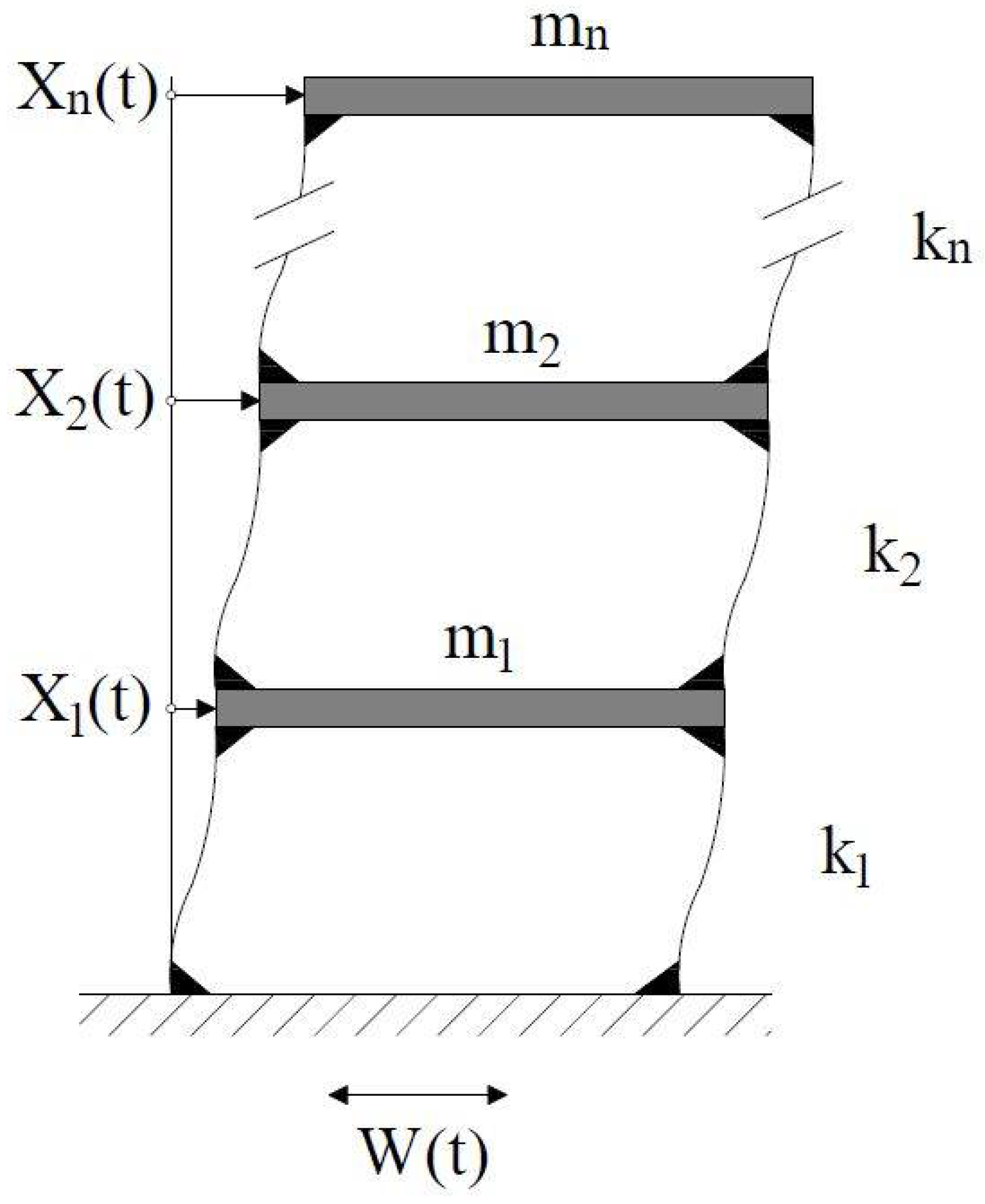
To validate the proposed method and to assess its reliability, several numerical simulations were performed on two MDoF classically damped systems: a 3DoF and a 5DoF shear-type frame. The general MDoF shear-type frame is depicted in Figure 2, and, for n = 3 and n = 5, it coincides with the aforementioned frames.

The 3DoF system has masses $m_1=2000\mathrm{kg}$, $m_2=1500\mathrm{kg}$, $m_3=1000\mathrm{kg}$; stiffness $k_1=24.72\times {10}^6\mathrm{N}/\mathrm{m}$, $k_2=12.36\times {10}^6\mathrm{N}/\mathrm{m}$, $k_3=11.124\times {10}^6\mathrm{N}/\mathrm{m}$; and damping ratios ${\zeta }_1=9.35\%$, ${\zeta }_2=9.06\%$, ${\zeta }_3=10.34\%$.

The 5DoF system is a frames have masses $m_1=m_2=10,000\mathrm{kg}$, $m_3=m_4=7500\mathrm{kg}$, $m_5=5000\mathrm{kg}$; stiffness $k_1=k_2=24.72\times {10}^6\mathrm{N}/\mathrm{m}$, $k_3=k_4=18.54\times {10}^6\mathrm{N}/\mathrm{m}$, $k_5=12.36\times {10}^6\mathrm{N}/\mathrm{m}$; and damping ratios ${\zeta }_1=8.04\%$, ${\zeta }_2=5.76\%$, ${\zeta }_3=6.44\%$, ${\zeta }_4=7.42\%$, ${\zeta }_5=8.10\%$.

The two structural systems are excited by a ground acceleration that is a white noise process with $S_0=4.7746\times {10}^{-3}{\mathrm{m}}^2/{\mathrm{s}}^3$. The number of samples considered is equal to 100, and the duration of each sample is equal to 60 s discretized with a sample frequency of 1000 Hz.

As far as the GA parameters are concerned, the maximum number of total generations chosen is 10,000, while the maximum number of stall generations and the value of $S_{0,\max }$ are, respectively, 400 and 0.5. The value of ${\epsilon }_f$ is equal to 5%, while ${\epsilon }_{\zeta }=50\%$. For the sake of clarity, the minimum and the maximum values of $f_j$ and ${\zeta }_j$ are reported in

Table 1. Minimum and maximum values of frequencies and damping ratios for the 3DoF case.

	${\mathit{f}}_1$	${\mathit{f}}_2$	${\mathit{f}}_3$	${\mathit{\zeta }}_1$	${\mathit{\zeta }}_2$	${\mathit{\zeta }}_3$
min	7.8238	19.0056	23.7068	0.0472	0.0453	0.0458
max	8.6474	21.0062	26.2023	0.1415	0.1360	0.1375

and

Table 2. Minimum and maximum values of frequencies and damping ratios for the 5DoF case.

	${\mathit{f}}_1$	${\mathit{f}}_2$	${\mathit{f}}_3$	${\mathit{f}}_4$	${\mathit{f}}_5$	${\mathit{\zeta }}_1$	${\mathit{\zeta }}_2$	${\mathit{\zeta }}_3$	${\mathit{\zeta }}_4$	${\mathit{\zeta }}_5$
min	2.4285	6.1453	9.3977	11.9656	13.6929	0.0414	0.0290	0.0319	0.0412	0.0189
max	2.6841	6.7922	10.3870	13.2252	15.1342	0.1241	0.0871	0.0957	0.1236	0.0568

, respectively, for the 3DoF system and the 5DoF system.

The results obtained with the proposed method are compared with those obtained by using two of the most popular OMA methods: FDD and SSI.

The discrepancies between the identified modal parameters and the exact ones, labelled as $\epsilon \%$, are calculated as

$$\epsilon \%=100\left|\frac{p^{\left(ex\right)}-p^{\left(id\right)}}{p^{\left(ex\right)}}\right|$$

(25)

in which $p^{\left(ex\right)}$ and $p^{\left(id\right)}$ represent, respectively, the exact modal parameters and the identified modal parameters.

In order to have a unique value that represents the reliability of the used methods, the FRF matrix of the system in nodal space is calculated as [5,62]

$$H^{\left(N\right)}\left(\omega \right)=\tilde{\mathsf{\Phi }}{H}^{\left(M\right)}\left(\omega \right){\tilde{\mathsf{\Phi }}}^T$$

(26)

where $H^{\left(M\right)}\left(\omega \right)$ is the FRF matrix in modal space that is a diagonal matrix whose components can be calculated with Equation (23). The discrepancy between the estimated FRF matrix in nodal space and the exact one is calculated as

$$\xi \%=\frac{100}{n_{dof}^2}{\displaystyle \sum _{i=1}^{n_{dof}}{\displaystyle \sum _{j=1}^{n_{dof}}\left(\frac{{\displaystyle \underset{0}{\overset{{\tilde{\omega }}_c}{\int }}\left|H_{ij}^{\left(N\right)}\left(\omega \right)-H_{ij}^{\left(N-ID\right)}\left(\omega \right)\right|d\omega }}{{\displaystyle \underset{0}{\overset{{\tilde{\omega }}_c}{\int }}\left|H_{ij}^{\left(N\right)}\left(\omega \right)\right|d\omega }}\right)}}$$

(27)

in which $H_{ij}^{\left(N\right)}\left(\omega \right)$ are the exact components of the FRF matrix in nodal space, $H_{ij}^{\left(N-ID\right)}\left(\omega \right)$ are the identified components of the FRF matrix, and $k_f={\tilde{\omega }}_c/\mathsf{\Delta }\omega$.

For the 3DoF system, the value of ${\tilde{\omega }}_c$ is equal to $2\pi \times 30$ rad/s, i.e., 30 Hz, while for the 5DoF frame, the value of ${\tilde{\omega }}_c$ is equal to $2\pi \times 24$ rad/s, i.e., 24 Hz.

A comparison was performed also in the time domain. Particularly, the systems identified by TAGA, SSI, and FDD and the exact systems were excited by a ground acceleration assumed as a white noise process. The response of each identified system was compared with the response of the exact system, the discrepancies ${\chi }_i\%$ being calculated as

$${\chi }_i\%=100\left(\frac{{\displaystyle \underset{0}{\overset{t_f}{\int }}\left|x_i^{\left(EX\right)}\left(t\right)-x_i^{\left(ID\right)}\left(t\right)\right|dt}}{{\displaystyle \underset{0}{\overset{t_f}{\int }}\left|x_i^{\left(EX\right)}\left(t\right)\right|dt}}\right)$$

(28)

in which $x_i^{\left(EX\right)}\left(t\right)$ is the i-th exact response, and $x_i^{\left(ID\right)}\left(t\right)$ is the i-th estimated response.

Since the GA can be applied in the same way to other OMA methods as well, it is possible to think that the choice to link the GA with another identification method is better than the one proposed. To clarify this, an additional comparison was performed. Particularly, the results obtained (in terms of FRF matrix identification) by applying TAGA on the 3DoF system are compared with those obtained by linking SSI with GA (SSI + GA).

To assess the robustness of the proposed method, additional numerical simulations were performed on the 3DoF system. Particularly, since the coefficients ${\epsilon }_f$ and ${\epsilon }_{\zeta }$ in Equations (15) and (16) and the maximum number of stall generation are quantities that must be defined by the user, four different couples of ${\epsilon }_f$ and ${\epsilon }_{\zeta }$ (${\epsilon }_f=5\%,{\epsilon }_{\zeta }=10\%$; ${\epsilon }_f=10\%,{\epsilon }_{\zeta }=20\%$; ${\epsilon }_f=20\%,{\epsilon }_{\zeta }=40\%$ and ${\epsilon }_f=5\%,{\epsilon }_{\zeta }=50\%$) were tested at different values of the maximum number of stall generations: 200; 400 and 800. Further, since in the real applications the value of $S_0$ can change, it was varied during the generation of the input process’ samples. Two different cases were analyzed, i.e., $S_0\in \left[{\tilde{S}}_0-0.1\times {\tilde{S}}_0,{\tilde{S}}_0+0.1\times {\tilde{S}}_0\right]$ and $S_0\in \left[{\tilde{S}}_0-0.2\times {\tilde{S}}_0,{\tilde{S}}_0+0.2\times {\tilde{S}}_0\right]$, where ${\tilde{S}}_0=4.7746\times {10}^{-3}{\mathrm{m}}^2/{\mathrm{s}}^3$. Another numerical simulation with 50 samples in which $S_0\in \left[{\tilde{S}}_0-0.2\times {\tilde{S}}_0,{\tilde{S}}_0+0.2\times {\tilde{S}}_0\right]$ was performed because the reduction of the number of samples produces, on the PSDs matrix of the structural output, effects that are similar to the addition of noise. In this way, it is possible to assess the reliability of the proposed method not only when there are fewer samples but also when instrumentation noise is present.

3. Results and Discussion

3.1. 3DoF System

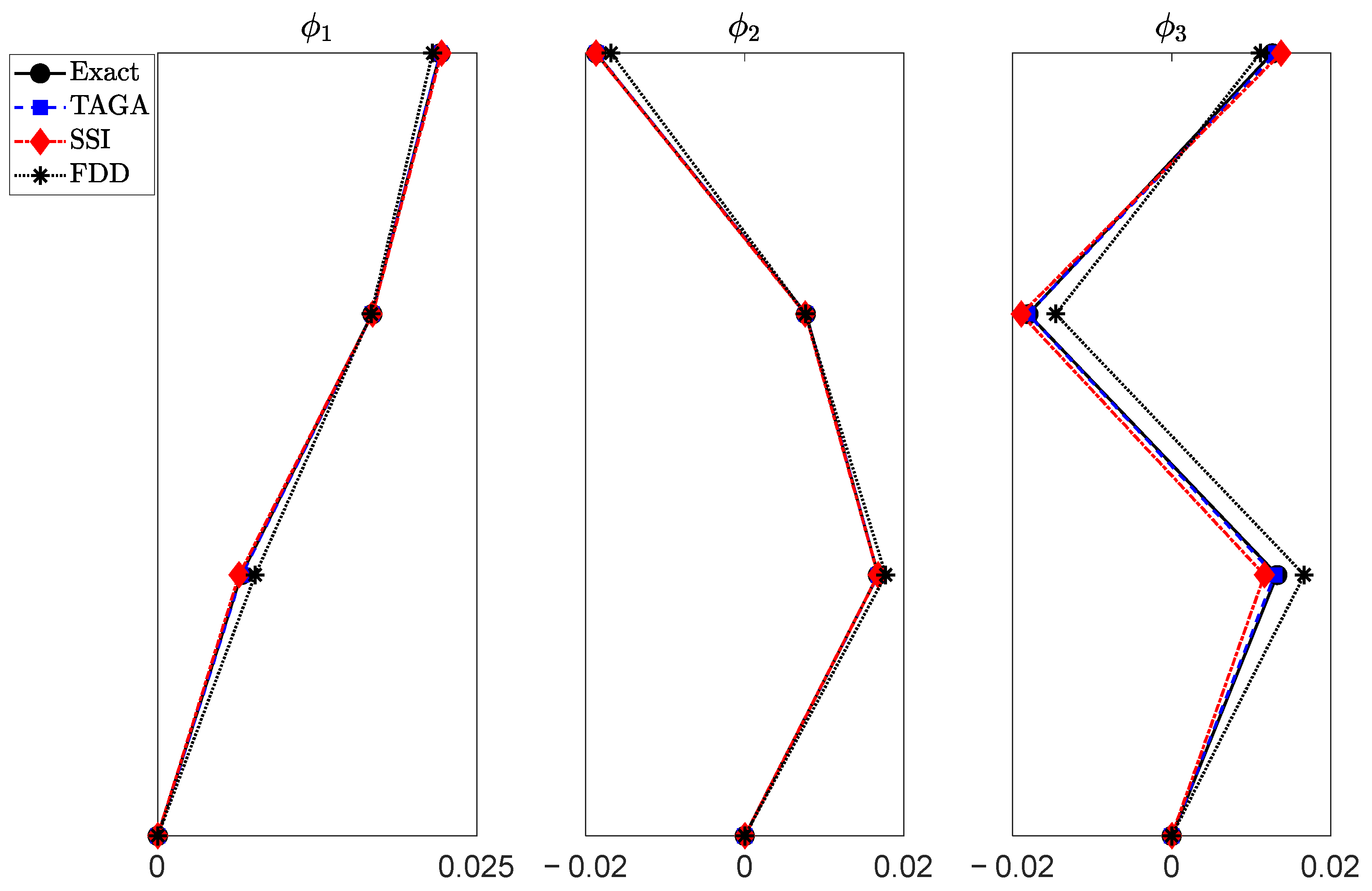
The results obtained with the proposed method and the other methods used are reported in

Table 3. Exact frequencies, identified frequencies, and corresponding discrepancies for the 3DoF system.

Mode	${\mathit{f}}_{\mathit{j}}^{\left(\mathit{e}\mathit{x}\right)}$	${\mathit{f}}_{\mathit{j}}^{\left(\mathit{T}\mathit{A}\mathit{G}\mathit{A}\right)}$	$\mathit{\epsilon }{\mathbf{\%}}^{\left(\mathit{T}\mathit{A}\mathit{G}\mathit{A}\right)}$	${\mathit{f}}_{\mathit{j}}^{\left(\mathit{S}\mathit{S}\mathit{I}\right)}$	$\mathit{\epsilon }{\mathbf{\%}}^{\left(\mathit{S}\mathit{S}\mathit{I}\right)}$	${\mathit{f}}_{\mathit{j}}^{\left(\mathit{F}\mathit{D}\mathit{D}\right)}$	$\mathit{\epsilon }{\mathbf{\%}}^{\left(\mathit{F}\mathit{D}\mathit{D}\right)}$
1	8.2363	8.2425	(0.0749)	8.2419	(0.0675)	8.0667	(2.0596)
2	19.9451	19.9455	(0.0022)	19.9645	(0.0977)	19.7083	(1.1869)
3	26.1214	26.1408	(0.0745)	26.0533	(0.2608)	25.9500	(0.6561)

and

Table 4. Exact damping ratios, identified damping ratios, and corresponding discrepancies for the 3DoF system.

Mode	${\mathit{\zeta }}_{\mathit{j}}^{\left(\mathit{e}\mathit{x}\right)}$	${\mathit{\zeta }}_{\mathit{j}}^{\left(\mathit{T}\mathit{A}\mathit{G}\mathit{A}\right)}$	$\mathit{\epsilon }{\mathbf{\%}}^{\left(\mathit{T}\mathit{A}\mathit{G}\mathit{A}\right)}$	${\mathit{\zeta }}_{\mathit{j}}^{\left(\mathit{S}\mathit{S}\mathit{I}\right)}$	$\mathit{\epsilon }{\mathbf{\%}}^{\left(\mathit{S}\mathit{S}\mathit{I}\right)}$	${\mathit{\zeta }}_{\mathit{j}}^{\left(\mathit{F}\mathit{D}\mathit{D}\right)}$	$\mathit{\epsilon }{\mathbf{\%}}^{\left(\mathit{F}\mathit{D}\mathit{D}\right)}$
1	0.0935	0.0940	(0.5287)	0.0941	(0.5996)	0.0951	(1.6872)
2	0.0906	0.0903	(0.3129)	0.0869	(4.0832)	0.0948	(4.7023)
3	0.1034	0.1026	(0.7509)	0.0993	(3.9518)	0.1716	(66.0030)

and Figure 3, respectively, for the frequencies, the damping ratios, and the modal shapes, the discrepancies $\epsilon \%$ being calculated as in Equation (25).

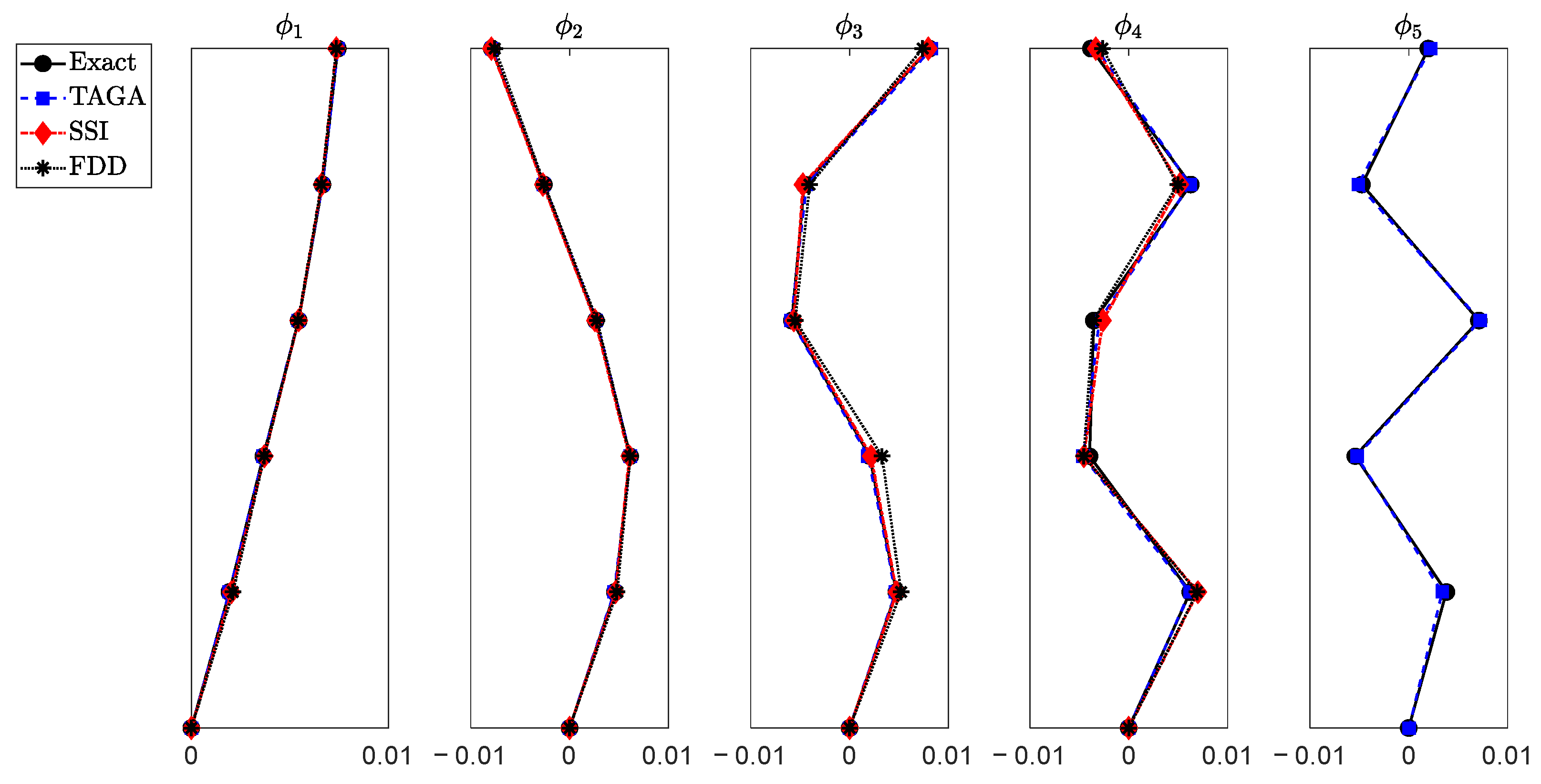
The results reported in Table 3 and Table 4 show that the proposed method reports very low discrepancies that are, in most cases, lower than those reported by the other methods. Furthermore, from the results reported in Figure 3, it is clear that the proposed method allows one to identify all the modal shapes with high accuracy.

The identified constant value of the PSD of the white noise $W\left(t\right)$ is $S_0=4.7754\times {10}^{-3}{\mathrm{m}}^2/{\mathrm{s}}^3$, and thus the discrepancy between the identified value and the exact value is equal to 0.0150%.

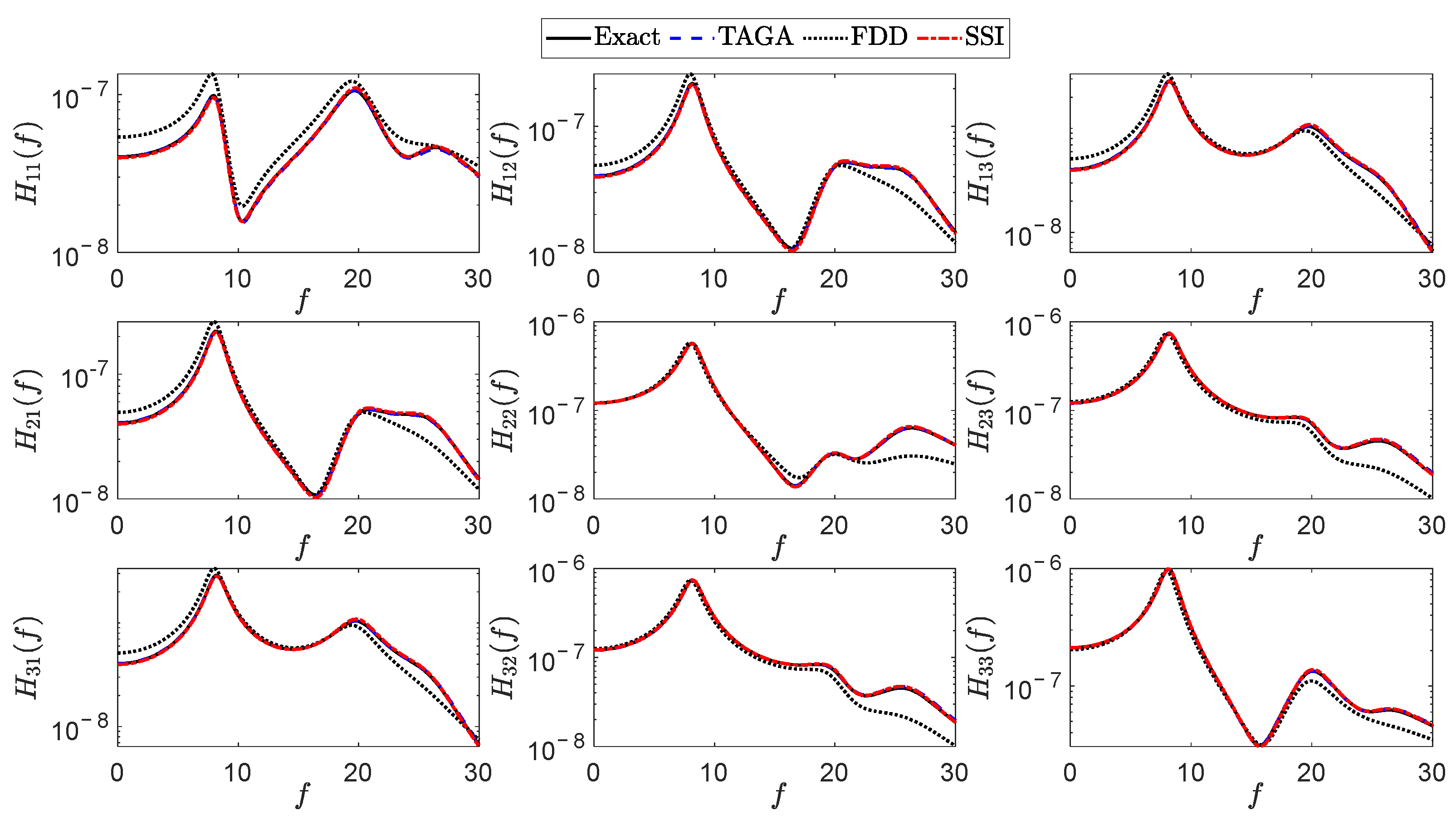
The discrepancy $\xi \%$ between the estimated FRF matrix and the exact one is calculated as in Equation (27). For each method used, it is reported in

Table 5. Discrepancy between the estimated FRFs matrix in nodal space and the exact one for the 3DoF system.

$\mathit{\xi }{\mathbf{\%}}^{\left(\mathit{T}\mathit{A}\mathit{G}\mathit{A}\right)}$	$\mathit{\xi }{\mathbf{\%}}^{\left(\mathit{S}\mathit{S}\mathit{I}\right)}$	$\mathit{\xi }{\mathbf{\%}}^{\left(\mathit{F}\mathit{D}\mathit{D}\right)}$
0.7505	1.6561	18.6879

.

The results reported in Table 5 show that the proposed method can identify the FRF matrix of the system with higher accuracy than the other methods. In Figure 4 the exact FRFs and the FRFs estimated with SSI, FDD, and TAGA are reported.

From the results reported in Figure 4, it can be seen that the proposed method can identify the FRF matrix with high precision.

The discrepancies ${\chi }_i\%$ between the structural outputs of the identified systems and the exact ones, calculated as in Equation (28), are reported in

Table 6. Discrepancy between the estimated structural responses and the exact ones for the 3DoF system.

Method	${\mathit{\chi }}_1\mathbf{\%}$	${\mathit{\chi }}_2\mathbf{\%}$	${\mathit{\chi }}_3\mathbf{\%}$
TAGA	4.4430	4.4883	4.5053
SSI	5.0563	4.6839	4.6478
FDD	29.1462	16.7604	16.2600

.

The results in Table 6 show that the proposed method leads to good results also in terms of prediction of the structural response.

The discrepancy between the FRF matrix estimated by using SSI + GA and the exact one, calculated as in Equation (27), is $\xi {\%}^{\left(SSI+GA\right)}=1.1375$; thus, linking SSI and GA is better than only using SSI. However, the best result is obtained through the use of the proposed method.

As far as the additional analyses performed at different values of ${\epsilon }_f$, ${\epsilon }_{\zeta }$ and the maximum number of stall generations are concerned, the results obtained show that a low value of the maximum number of stall generations (200) leads to good results only if the domain is small enough (${\epsilon }_f=5\%,{\epsilon }_{\zeta }=10\%$), while a high value (800) increases the computational burden without significantly improving the results. With 400 or 800 maximum stall generations, all the considered cases lead to good results that are very similar to each other; thus, the proposed method can be considered more reliable for high values of ${\epsilon }_{\zeta }$ provided that the maximum number of generations is not low. For ${\epsilon }_f$, a small value (5%) can be chosen to reduce the computational burden, since TD–ASM leads to good results in terms of frequency identification.

The discrepancy between the exact FRF matrix and the estimated FRF matrix, calculated by using Equation (27), is $\xi \%=0.9146$ and $\xi \%=0.9071$, respectively, for the cases $S_0\in \left[{\tilde{S}}_0-0.1\times {\tilde{S}}_0,{\tilde{S}}_0+0.1\times {\tilde{S}}_0\right]$ and $S_0\in \left[{\tilde{S}}_0-0.2\times {\tilde{S}}_0,{\tilde{S}}_0+0.2\times {\tilde{S}}_0\right]$. From these results it is clear that the modal parameters identified by using the proposed method always converge to results that are very similar to each other and that have very low discrepancies. Moreover, the discrepancies between the estimated values of ${\tilde{S}}_0$ and the exact ones are 0.1321% and 0.2173%, respectively, for the first and second cases.

Finally, the discrepancies $\xi \%$ calculated as in Equation (27) in the case $S_0\in \left[{\tilde{S}}_0-0.2\times {\tilde{S}}_0,{\tilde{S}}_0+0.2\times {\tilde{S}}_0\right]$ with 50 samples of the output process are $\xi {\%}^{\left(TAGA\right)}=1.2862$, $\xi {\%}^{\left(SSI\right)}=2.8976$, and $\xi {\%}^{\left(FDD\right)}=21.2477$, respectively, for TAGA, SSI, and FDD. These results show that even in this case, TAGA can identify the FRF matrix better than SSI and FDD. Thus, the proposed method can be considered reliable also in the case in which instrumentation noise is present. However, a method for the noise reduction consisting of filtering the PSDs of the structural output [4] can be applied before performing the identification in order to reduce the discrepancy.

3.2. 5DoF System

The proposed method was compared with SSI and FDD, and the results obtained from the numerical simulations on the 5DoF system are reported in

Table 7. Exact frequencies, identified frequencies, and corresponding discrepancies for the 5DoF system.

Mode	${\mathit{f}}_{\mathit{j}}^{\left(\mathit{e}\mathit{x}\right)}$	${\mathit{f}}_{\mathit{j}}^{\left(\mathit{T}\mathit{A}\mathit{G}\mathit{A}\right)}$	$\mathit{\epsilon }{\mathbf{\%}}^{\left(\mathit{T}\mathit{A}\mathit{G}\mathit{A}\right)}$	${\mathit{f}}_{\mathit{j}}^{\left(\mathit{S}\mathit{S}\mathit{I}\right)}$	$\mathit{\epsilon }{\mathbf{\%}}^{\left(\mathit{S}\mathit{S}\mathit{I}\right)}$	${\mathit{f}}_{\mathit{j}}^{\left(\mathit{F}\mathit{D}\mathit{D}\right)}$	$\mathit{\epsilon }{\mathbf{\%}}^{\left(\mathit{F}\mathit{D}\mathit{D}\right)}$
1	2.5626	2.5651	(0.0968)	2.5648	(0.0859)	2.5667	(0.1596)
2	6.4826	6.4755	(0.1089)	6.4792	(0.0531)	6.4750	(0.1172)
3	9.9069	9.9339	(0.2723)	9.9343	(0.2763)	9.8833	(0.2377)
4	12.8593	12.8822	(0.1785)	12.9408	(0.6339)	13.0000	(1.0945)
5	14.6603	14.6922	(0.2175)	-	(-)	-	(-)

and

Table 8. Exact damping ratios, identified damping ratios, and corresponding discrepancies for the 5DoF system.

Mode	${\mathit{\zeta }}_{\mathit{j}}^{\left(\mathit{e}\mathit{x}\right)}$	${\mathit{\zeta }}_{\mathit{j}}^{\left(\mathit{T}\mathit{A}\mathit{G}\mathit{A}\right)}$	$\mathit{\epsilon }{\mathbf{\%}}^{\left(\mathit{T}\mathit{A}\mathit{G}\mathit{A}\right)}$	${\mathit{\zeta }}_{\mathit{j}}^{\left(\mathit{S}\mathit{S}\mathit{I}\right)}$	$\mathit{\epsilon }{\mathbf{\%}}^{\left(\mathit{S}\mathit{S}\mathit{I}\right)}$	${\mathit{\zeta }}_{\mathit{j}}^{\left(\mathit{F}\mathit{D}\mathit{D}\right)}$	$\mathit{\epsilon }{\mathbf{\%}}^{\left(\mathit{F}\mathit{D}\mathit{D}\right)}$
1	0.0804	0.0846	(5.2219)	0.0861	(7.1421)	0.0871	(8.3413)
2	0.0576	0.0580	(0.8423)	0.0560	(2.7774)	0.0828	(43.8101)
3	0.0644	0.0653	(1.4107)	0.0602	(6.4419)	0.0739	(14.8178)
4	0.0742	0.0768	(3.4541)	0.0636	(14.2677)	0.0867	(16.8186)
5	0.0810	0.0568	(29.9094)	-	(-)	-	(-)

and Figure 5, respectively, for the frequencies, the damping ratios, and the modal shapes identification, the discrepancy $\epsilon \%$ being calculated by using Equation (25). The identified constant value of the PSD of the white noise input is $S_0=4.9871\times {10}^{-3}{\mathrm{m}}^2/{\mathrm{s}}^3$, and thus the discrepancy between the identified value and the exact value is equal to 4.4495%.

The results reported in Table 7 show that the proposed method leads to good results in terms of frequency identification, and that it allows one to identify the fifth natural frequency that is not identified by using FDD and SSI. From the results in Table 8, it is clear that the proposed method identifies the damping ratios better than the other methods, while from the results in Figure 5, it can be seen that the proposed method leads to good results also in terms of modal shape identification. Moreover, the proposed method, unlike the other methods, can identify also the fifth modal shape.

In order to establish which one of the methods used better approximates the global dynamic behavior of the structural system, the discrepancy between the estimated FRF matrix in nodal space and the exact one is calculated by using Equation (27), and the results are reported in

Table 9. Discrepancy between the estimated FRF matrix in nodal space and the exact one for the 5DoF system.

$\mathit{\xi }{\mathbf{\%}}^{\left(\mathit{T}\mathit{A}\mathit{G}\mathit{A}\right)}$	$\mathit{\xi }{\mathbf{\%}}^{\left(\mathit{S}\mathit{S}\mathit{I}\right)}$	$\mathit{\xi }{\mathbf{\%}}^{\left(\mathit{F}\mathit{D}\mathit{D}\right)}$
6.5106	14.8523	23.3143

.

As is shown in Table 9, once again TAGA can identify the FRF matrix of the system better than the other methods.

To evaluate the effectiveness of TAGA, SSI, and FDD in predicting the structural response, the discrepancies ${\chi }_i\%$ between the structural outputs of the identified systems and the exact ones were calculated as in Equation (28). The results are reported in

Table 10. Discrepancy between the estimated structural responses and the exact ones for the 5DoF system.

Method	${\mathit{\chi }}_1\mathbf{\%}$	${\mathit{\chi }}_2\mathbf{\%}$	${\mathit{\chi }}_3\mathbf{\%}$	${\mathit{\chi }}_4\mathbf{\%}$	${\mathit{\chi }}_5\mathbf{\%}$
TAGA	7.4555	7.4196	7.3487	7.2911	7.2426
SSI	8.0234	7.8052	7.7256	7.5996	7.5579
FDD	16.2492	16.4745	16.7753	16.8890	17.1428

.

They show that the structural response of the system identified by using the proposed method approximates the exact structural response in the time domain better than the response of the other identified systems, and thus TAGA can be considered reliable also in this regard.

4. Conclusions

In this paper, an innovative Operational Modal Analysis method for structural dynamic identification based on stochastic dynamics and signal analysis is proposed. It links the Time Domain–Analytical Signal Method with a Genetic Algorithm in order to identify the natural frequencies, the damping ratios, and the modal shapes of a structural system. The numerical simulations performed on 3DoF and 5DoF structural systems show that the method is reliable and that it can be used for the structural dynamic identification also when the structural damping is high. The Power Spectral Density of the structural excitation is identified with good accuracy, and the differences between the estimated and the exact system’s properties are very low, especially for the modes that have non-negligible modal mass. The discrepancy between the estimated Frequency Response Functions matrix and the exact one is less than those of the other methods used, and the results obtained in terms of structural response’s prediction are satisfying. For these reasons, the Time Domain–Analytical Signal Method with a Genetic Algorithm can be considered a reliable Operational Modal Analysis method that can be employed to easily perform Structural Health Monitoring in structural engineering applications.

References

- Zahid, F.B.; Ong, Z.C.; Khoo, S.Y. A review of operational modal analysis techniques for in-service modal identification. J. Braz. Soc. Mech. Sci. Eng. 2020, 42, 398. [Google Scholar] [CrossRef]
- Friis, T.; Tarpø, M.; Katsanos, E.I.; Brincker, R. Best linear approximation of nonlinear systems using Operational Modal Analysis. Mech. Syst. Signal Process. 2021, 152, 107395. [Google Scholar] [CrossRef]
- Zhang, L.; Brincker, R.; Andersen, P. An overview of operational modal analysis: Major development and issues. In Proceedings of the 1st International Operational Modal Analysis Conference, Copenhagen, Denmark, 26–27 April 2005. [Google Scholar]
- Bao, X.X.; Li, C.L.; Xiong, C.B. Noise elimination algorithm for modal analysis. Appl. Phys. Lett. 2015, 107, 041901. [Google Scholar] [CrossRef]
- Rainieri, C.; Fabbrocino, G. Operational Modal Analysis of Civil Engineering Structures: An Introduction and Guide for Applications, 1st ed.; Springer: New York, NY, USA, 2014. [Google Scholar] [CrossRef]
- Mottershead, J.E.; Link, M.; Friswell, M.I. The sensitivity method in finite element model updating: A tutorial. Mech. Syst. Signal Process. 2011, 25, 2275–2296. [Google Scholar] [CrossRef]
- Zare, H.G.; Maleki, A.; Rahaghi, M.I.; Lashgari, M. Vibration modelling and structural modification of combine harvester thresher using operational modal analysis and finite element method. Struct. Monit. Maint. 2019, 6, 33–46. [Google Scholar] [CrossRef]
- Diaz, I.M.; Pereira, E.; Reynolds, P. Integral resonant control scheme for cancelling human-induced vibrations in light-weight pedestrian structures. Struct. Control Health Monit. 2012, 19, 55–69. [Google Scholar] [CrossRef]
- Jones, C.; Reynolds, P.; Pavic, A. Vibration serviceability of stadia structures subjected to dynamic crowd loads: A literature review. J. Sound Vib. 2011, 330, 1531–1566. [Google Scholar] [CrossRef]
- Gentile, C.; Saisi, A.E. OMA-based structural health monitoring of historic structures. In Proceedings of the 8th International Operational Modal Analysis Conference, Copenhagen, Denmark, 13–15 May 2019. [Google Scholar]
- Ubertini, F.; Comanducci, G.; Cavalagli, N. Vibration-based structural health monitoring of a historic bell-tower using output-only measurements and multivariate statistical analysis. Struct. Health Monit. 2016, 15, 438–457. [Google Scholar] [CrossRef]
- Westerkamp, C.; Hennewig, A.; Speckmann, H.; Bisle, W.; Colin, N.; Rafrafi, M. An Online System for Remote SHM Operation with Content Adaptive Signal Compression. In Proceedings of the 7th European Workshop on Structural Health Monitoring, Nantes, France, 8–11 July 2014. [Google Scholar]
- Rainieri, C.; Fabbrocino, G.; Cosenza, E. Fully automated OMA: An opportunity for smart SHM systems. In Proceedings of the XXVII International Modal Analysis Conference, Orlando, FL, USA, 9–12 February 2009. [Google Scholar]
- Di Matteo, A.; Fiandaca, D.; Pirrotta, A. Smartphone-based bridge monitoring through vehicle-bridge interaction: Analysis and experimental assessment. J. Civ. Struct. Health Monit. 2022; in press. [Google Scholar]
- Magalhães, F.; Cunha, A.; Caetano, E. Vibration based structural health monitoring of an arch bridge: From automated OMA to damage detection. Mech. Syst. Signal Process. 2012, 28, 212–228. [Google Scholar] [CrossRef]
- Shimpi, V.; Sivasubramanian, M.; Singh, S. System Identification of Heritage Structures through AVT and OMA: A Review. Struct. Durab. Health Monit. 2019, 13, 1–40. [Google Scholar] [CrossRef]
- Di Matteo, A.; Masnata, C.; Russotto, S.; Bilello, C.; Pirrotta, A. A novel identification procedure from ambient vibration data. Meccanica 2021, 56, 797–812. [Google Scholar] [CrossRef]
- Russotto, S.; Di Matteo, A.; Masnata, C.; Pirrotta, A. OMA: From research to engineering applications. Lect. Notes Civ. Eng. 2021, 156, 903–920. [Google Scholar] [CrossRef]
- Ubertini, F.; Gentile, C.; Materazzi, A.L. Automated modal identification in operational conditions and its application to bridges. Eng. Struct. 2013, 46, 264–278. [Google Scholar] [CrossRef]
- Peeters, B.; Ventura, C. Comparative study of modal analysis techniques for bridge dynamic characteristics. Mech. Syst. Signal Process. 2003, 17, 965–988. [Google Scholar] [CrossRef]
- Brownjohn, J.; Magalhaes, F.; Caetano, E.; Cunha, A. Ambient vibration re-testing and operational modal analysis of the Humber Bridge. Eng. Struct. 2010, 32, 2003–2018. [Google Scholar] [CrossRef] [Green Version]
- Standoli, G.; Giordano, E.; Milani, G.; Clementi, F. Model Updating of Historical Belfries Based on Oma Identification Techniques. Int. J. Archit. Herit. 2021, 15, 132–156. [Google Scholar] [CrossRef]
- Darbre, G.; De Smet, C.; Kraemer, C. Natural frequencies measured from ambient vibration response of the arch dam of Mauvoisin. Earthq. Eng. Struct. Dyn. 2000, 29, 577–586. [Google Scholar] [CrossRef]
- Brownjohn, J. Long-term monitoring of dynamic response of a tall building for performance evaluation and loading characterisation. In Proceedings of the 1st International Operational Modal Analysis Conference, Copenhagen, Denmark, 26–27 April 2005. [Google Scholar]
- Kim, D.; Oh, B.K.; Park, H.S.; Shim, H.B.; Kim, J. Modal Identification for High-Rise Building Structures Using Orthogonality of Filtered Response Vectors. Comput. Aided Civ. Infrastruct. 2017, 32, 1064–1084. [Google Scholar] [CrossRef]
- Bajrić, A.; Høgsberg, J.; Rüdinger, F. Evaluation of damping estimates by automated operational modal analysis for offshore wind turbine tower vibrations. Renew. Energy 2018, 116, 153–163. [Google Scholar] [CrossRef] [Green Version]
- Brincker, R.; Andersen, P.; Martinez, M.; Tallavo, F. Modal analysis of an offshore platform using two different ARMA approaches. In Proceedings of the 14th International Modal Analysis Conference, Dearborn, Michigan, 12–15 February 1996. [Google Scholar]
- Brownjohn, J.M.W.; Carden, E.; Goddard, C.; Oudin, G. Real-time performance monitoring of tuned mass damper system for a 183 m reinforced concrete chimney. J. Wind Eng. Ind. Aerodyn. 2010, 98, 169–179. [Google Scholar] [CrossRef]
- Dooms, D.; Degrande, G.; De Roeck, G.; Reynders, E. Finite element modelling of a silo based on experimental modal analysis. Eng. Struct. 2006, 28, 532–542. [Google Scholar] [CrossRef]
- Peeters, B.; Van der Auweraer, H.; Vanhollebeke, F.; Guillaume, P. Operational modal analysis for estimating the dynamic properties of a stadium structure during a football game. Shock. Vib. 2007, 14, 283–303. [Google Scholar] [CrossRef]
- Bendat, J.; Piersol, A. Engineering Applications of Correlation and Spectral Analysis, 2nd ed.; Wiley: New York, NY, USA, 1993. [Google Scholar]
- Brincker, R.; Zhang, L.; Andersen, P. Modal Identification from Ambient Responses using Frequency Domain Decomposition. In Proceedings of the 18th International Modal Analysis Conference, San Antonio, TX, USA, 7–10 February 2000. [Google Scholar]
- Brincker, R.; Zhang, L.; Andersen, P. Output-Only Modal Analysis by Frequency Domain Decomposition. In Proceedings of the International Conference on Noise and Vibration Engineering, Leuven, Belgium, 13–15 September 2000. [Google Scholar]
- Brincker, R.; Ventura, C.; Andersen, P. Damping estimation by frequency domain decomposition. In Proceedings of the 19th International Modal Analysis Conference, Kissimmee, FL, USA, 5–8 February 2001. [Google Scholar]
- James, G.H.; Carne, T.G.; Laufer, J. The natural excitation technique (NExT) for modal parameter extraction from operating structures. Int. J. Anal. Exp. Modal Anal. 1995, 10, 260–277. [Google Scholar]
- Juang, J.-N.; Pappa, R.S. An eigensystem realization algorithm for modal parameter identification and model reduction. J. Guid. Control Dyn. 1985, 8, 620–627. [Google Scholar] [CrossRef]
- Vold, H.; Kundrat, J.; Rocklin, G.T.; Russell, R. A multi-input modal estimation algorithm for mini-computers. SAE Trans. 1982, 91, 815–821. [Google Scholar] [CrossRef]
- Fukuzono, K. Investigation of Multiple-Reference Ibrahim Time Domain Modal Parameter Estimation Technique. Master’s Thesis, University of Cincinnati, Cincinnati, OH, USA, 1986. [Google Scholar]
- Andersen, P. Identification of Civil Engineering Structures Using Vector ARMA Models. Ph.D. Thesis, Aalborg University, Aalborg, Danmark, 1997. [Google Scholar]
- Andersen, P.; Brincker, R.; Kirkegaard, P.H. Theory of covariance equivalent ARMAV models of civil engineering structures. In Proceedings of the 14th International Modal Analysis Conference, Dearborn, Michigan, 12–15 February 1996. [Google Scholar]
- Ljung, L. System Identification—Theory for the User; Prentice-Hall: Englewood Cliffs, NJ, USA, 1987. [Google Scholar]
- Petsounis, K.; Fassois, S. Parametric time-domain methods for the identification of vibrating structures—a critical comparison and assessment. Mech. Syst. Signal Process. 2001, 15, 1031–1060. [Google Scholar] [CrossRef]
- Kim, B.H.; Stubbs, N.; Park, T. A new method to extract modal parameters using output-only responses. J. Sound Vib. 2005, 282, 215–230. [Google Scholar] [CrossRef]
- De Moor, B.; Van Overschee, P.; Suykens, J. Subspace algorithm for system identification and stochastic realization. In Proceedings of the International Symposium on the Mathematical Theory of Networks and Systems, Kobe, Japan, 17–21 June 1991. [Google Scholar]
- Peeters, B.; De Roeck, G. Reference-based Stochastic Subspace Identification for Output-Only Modal Analysis. Mech. Syst. Signal Process. 1999, 13, 855–878. [Google Scholar] [CrossRef] [Green Version]
- Qin, S.; Kang, J.; Wang, Q. Operational modal analysis based on subspace algorithm with an improved stabilization diagram method. Shock. Vib. 2016, 2016, 7598965. [Google Scholar] [CrossRef] [Green Version]
- Van Overschee, P.; De Moor, B. Subspace algorithms for the stochastic identification problem. Automatica 1993, 29, 649–660. [Google Scholar] [CrossRef]
- Cottone, G.; Pirrotta, A.; Salamone, S. Incipient Damage Identification through Characteristics of the Analytical Signal Response. Struct. Control Health Monit. 2008, 15, 1122–1142. [Google Scholar] [CrossRef]
- Lo Iacono, F.; Navarra, G.; Pirrotta, A. A Damage Identification procedure based on Hilbert transform: Experimental validation. Struct. Control Health Monit. 2012, 19, 146–160. [Google Scholar] [CrossRef] [Green Version]
- Barone, G.; Marino, F.; Pirrotta, A. Low stiffness variation in structural systems: Identification and localization. Struct. Control Health Monit. 2008, 15, 450–470. [Google Scholar] [CrossRef]
- Avci, O.; Abdeljaber, O.; Kiranyaz, S.; Hussein, M.; Gabbouj, M.; Inman, D.J. A review of vibration-based damage detection in civil structures: From traditional methods to Machine Learning and Deep Learning applications. Mech. Syst. Signal Process. 2021, 147, 107077. [Google Scholar] [CrossRef]
- Gui, G.; Pan, H.; Lin, Z.; Li, Y.; Yuan, Z. Data-driven support vector machine with optimization techniques for structural health monitoring and damage detection. J. Civ. Eng. 2017, 21, 523–534. [Google Scholar] [CrossRef]
- Avci, O.; Abdeljaber, O.; Kiranyaz, S.; Inman, D.J. Structural health monitoring with self-organizing maps and artificial neural networks. In Proceedings of the 37th International Modal Analysis Conference (IMAC XXXVII), Orlando, FL, USA, 28–31 January 2019. [Google Scholar]
- Abdeljaber, O.; Avci, O. Nonparametric structural damage detection algorithm for ambient vibration response: Utilizing artificial neural networks and self-organizing maps. J. Archit. Eng. 2016, 22, 04016004. [Google Scholar] [CrossRef]
- Santos, A.; Figueiredo, E.; Silva, M.F.M.; Sales, C.S.; Costa, J.C.W.A. Machine learning algorithms for damage detection: Kernel-based approach. J. Sound Vib. 2016, 363, 584–599. [Google Scholar] [CrossRef]
- Mitchell, M. An Introduction to Genetic Algorithms; MIT Press: Cambridge, MA, USA, 1996. [Google Scholar]
- Vose, M.D. The Simple Genetic Algorithm: Foundations and Theory; MIT Press: Cambridge, MA, USA, 1999. [Google Scholar]
- Xiang, J.; Zhong, Y.; Chen, X.; He, Z. Crack detection in a shaft by combination of wavelet-based elements and genetic algorithm. Int. J. Solids Struct. 2008, 45, 4782–4795. [Google Scholar] [CrossRef] [Green Version]
- Tran-Ngoc, H.; Khatir, S.; De Roeck, G.; Bui-Tien, T.; Nguyen-Ngoc, L.; Abdel Wahab, M. Model Updating for Nam O Bridge Using Particle Swarm Optimization Algorithm and Genetic Algorithm. Sensors 2018, 18, 4131. [Google Scholar] [CrossRef] [Green Version]
- Welch, P.D. The use of fast Fourier transform for the estimation of power spectra: A method based on time averaging over short, modified periodograms. IEEE Trans. Audio Electroacoust. 1967, 15, 70–73. [Google Scholar] [CrossRef] [Green Version]
- Barbe, K.; Pintelon, R.; Schoukens, J. Welch Method Revisited: Nonparametric Power Spectrum Estimation Via Circular Overlap. IEEE Trans. Signal Process. 2010, 58, 553–565. [Google Scholar] [CrossRef]
- Muscolino, G. Dinamica Delle Strutture; McGraw-Hill: Milano, Italy, 2002. [Google Scholar]
Figure 1.
Classical GA scheme.
Figure 2.
General MDoF shear-type frame used for the numerical simulations.
Figure 3.
Comparison between the identified modal shapes and the exact ones for the 3DoF system.
Figure 4.
Comparison between the identified FRFs and the exact ones.
Figure 5.
Comparison between the identified modal shapes and the exact ones for the 5DoF system.