
Analytical Implications of Mortgage Lending Value and Bottom Value
by
 and
and
Francesca Salvo
1, 
Manuela De Ruggiero
1, 
Daniela Tavano
1, 
Pierfrancesco De Paola
2,* and
Francesco Paolo Del Giudice
3,*
1
Department of Environmental Engineering, University of Calabria, Pietro Bucci St., 87036 Rende, Italy
2
Department of Industrial Engineering, University of Naples “Federico II”, Vincenzo Tecchio Sq. 80, 80125 Naples, Italy
3
Department of Architecture and Design, University of Rome “Sapienza”, Borghese Sq. 9, 00186 Rome, Italy
*
Authors to whom correspondence should be addressed.
Buildings 2022, 12(6), 799; https://doi.org/10.3390/buildings12060799
Submission received: 17 March 2022
/
Revised: 2 June 2022
/
Accepted: 7 June 2022
/
Published: 10 June 2022
(This article belongs to the Section Architectural Design, Urban Science, and Real Estate)
Abstract
:This study concerns the analytical formulation and relative implications of bottom value (BV) and mortgage lending value (MLV) regarding properties where the existing building provides an income during its useful life, leaving thereafter only the land value. The bottom value is equal to the overall property’s market value minus all incomes not collected by the end of the building’s economic life. Furthermore, it considers the income rates for land and buildings differently according to the investment type, while the mortgage lending value considers, instead, a unique rate. The mortgage lending value assessment is conducted under restrictive assumptions on long-term aspects, future marketability, and local market conditions. For the first time, mathematical and appraisal models have been applied to determine the mortgage lending value and the bottom value in particular cases, such as that mentioned above and considered in the present study (existing buildings providing income during their useful life). Some of the indexes introduced in the paper are completely original with respect to the current reference literature.
1. Introduction
The mortgage lending value (MLV) is not a term universally understood or accepted. The European Banking Authority (EBA) has the mandate to develop a draft of the Regulatory Technical Standards (RTS) to specify the rigorous criteria for MLV assessment [1]. The mortgage lending value (MLV) is different from the mortgage value (MV) because they are calculated using different methods. The purpose of MLV is to provide a long-term and sustainable value to judge the suitability of a property for a reliable and secure mortgage. Then, MLV is designed to be robust against market fluctuations. The most substantial and principal difference between MLV and MV is that the first is intended to be a property value assessment for a long period of time and theoretically realizable in a sale at any point in time during the loan period; instead, the MV is an assessment at a given moment in time (specific valuation date). The MLV is well below the market value because it does not consider the market fluctuations and settles down to the minimum value that the property assumes throughout the terms of a mortgage. The valuation of loan security, mortgages, and debentures for lending institutions and other providers is typically dealt with periodically by referring to the concept of MV when specific assets to secure financing are evaluated. Valuers may occasionally deal with the non-market value basis, such as going-concern value, liquidation value, or other types of values depending on laws, circumstances, and the secured party’s requirements, but those who supply financing are most concerned with MV. Other types of values depend on laws, circumstances, and the secured party’s requirements [2].
The aim of this paper is to propose an analytical formulation of the bottom value (BV) and mortgage lending value (MLV), starting with the following hypotheses:
- The property income is equal to the sum of land income and building income;
- The land’s income is independent of the property usage;
- The incomes are levelled in time (land and property) in accordance with the estimative principle of the “Permanence of the Conditions”;
- The cost and time implications of building demolition are negligible.
This paper consists of four sections. In Section 2, a literature review on the subject and the legislative and institutional state of the art is provided. In Section 3, we deliver the methodological structure on which the appraisal of the market value of a built property, the land and building values, the incidence of built area and its income, and the capitalization rate are based. In Section 3.1, a hypothesis of practical interest is studied dealing with the calculation of the BV of a property in which the existing building provides income for the duration of its economic life, beyond which the income is provided by the land, which is considered the minimum cash flow. In Section 3.2, we introduce a series of expressions that represent the ability to calculate the MLV by referring to the discount rate of the market value calculated through ratios and financial terms as well as the market. In Section 4, the results and discussion are presented. The relationships between market value, BV, and MLV, together with their notable relations, are illustrated. Finally, in Section 5, the contributions of this study are summarized.
2. Literature Review
Mortgage valuation (MV) is a topic widely discussed in German literature mostly. In particular, Ross and Brachmann [3], Sommer and Kroll [4], and Rossler and Langner [5] have dealt with this topic extensively. Contents and approaches to MV methods are very similar in these publications with national applicability. The study of Metzner [6] and Adolf [7] only marginally covers this research area. More specific studies aiming to analyze the MLV were conducted by Werth [8], Ruchardt [9], Stocker [10], and Kierig [11].
In the Anglo-American journals about property valuation and lending, relevant studies are attributable to Crosby and French [12], White and Turner [13], Serret and Trello [14], Adair and Hutchison [15], and Joslin [16]. Among other issues, issues related to the valuation quality, the macroeconomic impact, or the exertion of influence of banks on the valuation results are also dealt with, as in Crosby et al. [17], Bretten and Wyatt [18], Ciuna et al. [19], Bienert [20], and Pitschke [21]. Often, these works are particularly interesting and relevant within the boundaries of the countries considered.
On a macroeconomic level, in 1994, Renaud worked on questions concerning real estate cycles, property risk, credit crunch, and cause and effect chains within the real estate industry [22]. The findings of Maier [23], Ropeter [24], Wüstefeld [25], and Pfnür and Armonat [26] related to property risk identification and assessment are of great interest, particularly for German real estate markets. The results of PriceWaterhouseCoopers (PWC, [27]), as well as Milleker [28] or Tsatsaronis [29], concerning the determinants of real estate prices are also significant. Otherwise, the works of Jorion [30] and Poppensieker [31] are centered around risk assessment in general. French and Gabrielli [32] define risk as the measure of the difference between actual and expected outcomes of the analysis, whereas uncertainty concerns the lack of knowledge and poor or imperfect information about the inputs required in the model. Benvenuti [33] proposes a calculation criterion for the MLV determination that originates from the financial method application (direct capitalization) by adopting a capitalization rate calculated by means of the debt coverage ratio (DCR).
A more recent study by Tajani and Morano [34] proposes and tests an innovative methodology for assessing MLV, trying to improve and rationalize the appraisal of the percentage reduction to be applied to the market value.
With reference to aspects of mortgage lending from a bankʹs point of view and the interaction of European mortgage markets especially, to highlight there are the works of Süchting [35], Rode [36], Ruchardt [9,37], Paschedag [38], Steffan and Scholz [39], Low et al. [40]. Gondring and Lorenz [41] affirm that the MLV must be conceived as an independent value which is not identical to the market value.
International studies show that the relationship between the MV and how the MLV should be calculated is still unclear [42].
European legislation, following the Basel agreements on the regulation of the banking system, on several occasions has addressed the problem of mortgage guarantees and the associated risks of non-performing banks in the event of debtor’s insolvency, starting from the indications contained in the EU Directive 98/32/EC of the European Parliament and Council of 22 June 1998 [43]. This Directive defines the MLV as follows: “the value of the property as determined by a valuer making a prudent assessment of the future marketability of the property by taking into account long-term sustainable aspects of the property, the normal and local market conditions, the current use and alternative appropriate uses of the property. Speculative elements shall not be taken into account in the assessment of the mortgage lending value. The mortgage lending value shall be documented in a transparent and clear manner”. This Directive was followed by the Directive 2006/48/EC, then replaced by 2013/36/EU, with a view to regulating and harmonizing the regulatory framework for the granting of credit against collateral.
As a result, the main European organizations responsible for drawing up standards for property valuation had to take account of the principles and concepts expressed in European legislation on property valuation, integrating them into their doctrinal corpus and framing them according to the principles of the estimative doctrine and the standard methodologies of evaluation already consolidated.
The European Parliament defines the guidelines to which the international standards adhere: the “White Book” of the IVSC (International Valuation Standard Council), the “Blue Book” of the EVS (European Valuation Standards) of the TEGoVA (The European Group of Valuers’Associations) and the Appraisal and Valuation Manual known as “Red Book” of the RICS (Royal Institution of Chartered Surveyors).
The European Mortgage Federation (EMF) states that the MLV cannot be grouped with other valuation approaches based on MV that are taken on a given date, while the MLV is estimated to verify if a mortgaged property provides sufficient guarantee to secure a loan over a long period and thus reflects the long-term value of a property.
The TEGoVA is the first institution to adopt this definition and integrate it with the EVS. In its European Valuation Standards, TEGoVA defines the MLV as a valuation basis other than MV. This concept is reproduced even in the most recent edition of the 2020 European Valuation Standards [44], where the MLV is defined as follows: “The value of immovable property as determined by a prudent assessment of the future marketability of the property taking into account long-term sustainable aspects of the property, the normal and local market conditions, the current use and alternative appropriate uses of the property”. The above definition was incorporated into Capital Requirements Regulation (EU) No. 575/2013, art. 4 (74) [45].
The European Banking Authority (EBA) has identified the need to apply the MLV and reach a harmonization of rigorous criteria for the respective valuation [1].
The International Valuation Standard Council (IVSC) defines the MLV as a non-market value basis in the International Valuation Standards (IVS 2), highlighting that the MLV “is a value concept used for property lending purposes, based on the sustainable aspects of the property and restricting the assessment of property value to the permanent economic characteristics of the property and the revenue that any tenant could produce by proper management” [2]. With this value, they refer to market risks (present market conditions, market cycles, market volatility, stability, liquidity, demographic trend, attractiveness of regional markets, etc.), location risks (suitability of the location for investment, revenues and increases in values, infrastructure, micro-trend of the local economy, etc.), construction-related property risks (physical, quality of the property, maintenance requirements, reconstruction costs, etc.), risks related to the tenants and leases, fiscal risks (current tax situation, potential positive or negative changes, etc.), and legal risks (ownership, planning permission, subside, etc.).
3. Methodological Structure of the Model
In the traditional real estate appraisal methods, the market value of a built property can ideally be decomposed into the sum of the land market value (without buildings) and the building’s market value. Thus, in analytical terms:
where V is the market value of a built property, calculated by adding the land value VL to the building value VB. This relationship sets a clear separation between the land property and the building property that ideally are supposed to provide separate incomes.
The incidence of the built area is the ratio of the land value to the real estate property value:
By analogy with Formula (1), the market income R of a built property is also equal to the sum of the income of the built area and the income of the building:
The real estate net income is obtained by subtracting the operating expenses—normally to be covered by the landlord—from the real estate gross income. The individual cost items are management costs, maintenance costs, loss of rental income risk, and any other running costs not covered by allocable shares in costs. The costs include a modernization risk specific to the property type. The operating expenses of the property would include expenses for legal and accounting, insurance, janitorial, supplies, taxes, utilities, etc. They also include principal and interest payments on loans, capital expenditures, and depreciation. According to the Regulation on the Determination of the MLV of Properties in accordance with § 16 pars. 1 and 2 of the Pfandbrief Act, the minimum amount of a deduction of operating expenses must equal at least 15 percent of the gross income [8,9,10,11]. The capitalization rate must reflect long-term market trends and exclude all short-term expectations regarding the return on investment of the property. A specific section of the BelWertV also stipulates the capitalization rate [8,9,10,11]. In the case of residential properties, it must be at least 5% and at least 6% for commercially used properties (or, in exceptional cases, i.e., prime commercial properties, at least 5.5%).
The income of the original built area refers to the pure rent. The built land income () expresses the ratio of land income to property income:
The building income is referred to the rent due to its owner, and can be calculated as a complement to one of the incidences of the land income:
The land value can be appraised with the direct capitalization method or by capitalizing the land income with the land capitalization rate as follows:
Land value and income are reflected, respectively, in the market segment of the built areas and in that of the property use. Building value appraisal can be represented with the direct capitalization method or capitalizing the building income with the building capitalization rate as follows:
Investment in land presents less risk than investment in building, unlimited duration, potential revaluation, and lower management costs, assuming the same advantages and disadvantages for the land. Investments in buildings present increasing risks in the medium–long term, potential building depreciation, and higher management and administration costs, assuming the same advantages and disadvantages for the building [46,47,48,49,50,51,52,53].
The capitalization rate r of the property according to the same investment type is equal to:
where is the incidence of the built land.
The residual techniques are based on this type of analysis. According to Formula (1), the market value of the property, replacing Formulas (6) and (7), is equal to:
The relationship between the land incidence and the income incidence can be presented in the following way:
for , we have . Once the incidence of the land is known, the incidence of income is derived from Formula (10):
For , we have , which means that the impact of the land capitalization rate is equal to the incidence of income.
The applied direct capitalization method considers the incomes and the rates instantly, without a temporal implication in the cash flow of the property and of its component parts. If one interprets the pattern of Formula (1) in terms of cash flow, this can be represented by the income of the property (land and building) as constant and unlimited in time; the underlying hypothesis considers the maintenance of the current situation in the long term, considering any demolitions and reconstructions of the building (on the spot) at the end of its economic life and fixing demolition and construction costs equal to the building value. The permanence of these conditions requires the highest and best use constant for the property. To estimate the property market value, these assumptions are not necessary if comparable incomes and property prices are collected directly from the real estate market.
3.1. Existing Use of the Property
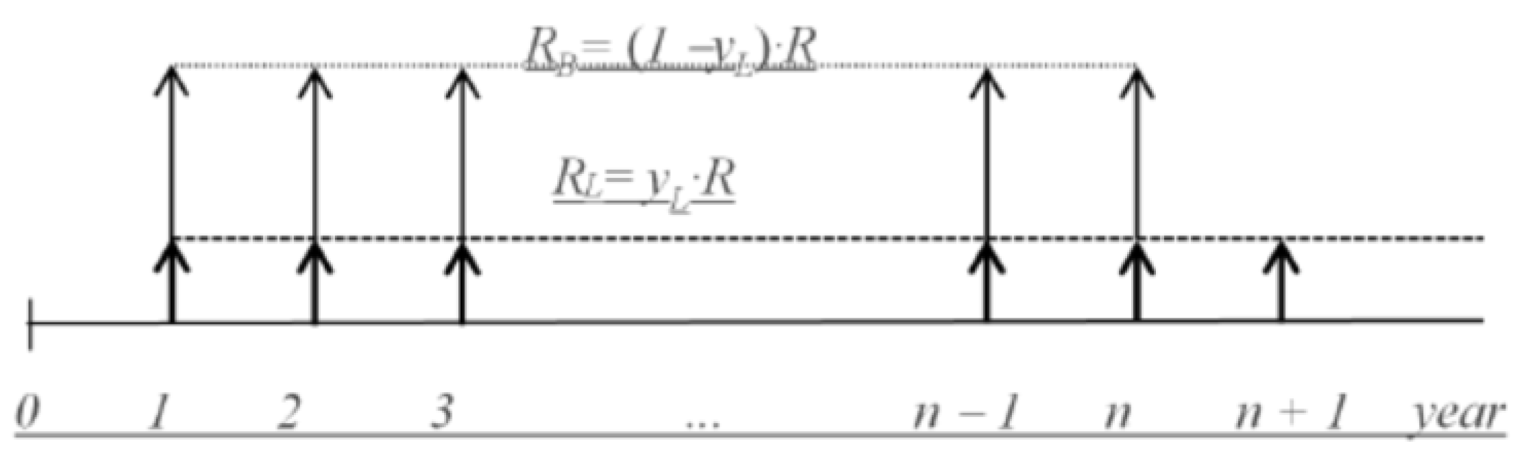
A hypothesis of practical interest is that of a property in which the existing building provides an income for the duration of its economic life, after which it leaves only the land as residual real estate good. The latter represents the lowest assumption based on the existing use of the property, for which the building provides temporary income with reference to market realities and to certain purposes (Figure 1). For a built property, this is the most restrictive assumption. The market value and the non-market value of the property are equal to the present value of the minimum cash flow. The current value represents the bottom value that, according to Formula (1), is equal to the sum of the land value and the building value , which refers to the residual economic life of the building, in the following way:
The appraisal of the building value is made by capitalizing the income of the building for the expected remaining useful life n with the building capitalization rate, as follows:
The bottom value V* can be proposed in relation to the land incidence according to Formula (12), replacing Formulas (6) and (13), as follows:
and in relation to the income incidence, as follows:
The bottom value is also equal to the property market value (building and land) from Formula (9) minus the present value of the building income not collected at the end of its economic life. The bottom value can be calculated by considering the impact of the land as follows:
and considering the income incidence as follows:
The calculation of the bottom value related to the incidence of land income is appropriate when the incidence can be estimated independently as in-built areas. Therefore, the bottom value can be appraised with methods based on market value.
In general, the term “bottom value” originates from the typical fluctuations of the financial markets: a bottom is the lowest value or price traded or published by financial security, commodity, or index within a particular referenced time frame. However, in financial studies, this term often refers to a significant low point of interest. A price or value bottom is referenced for a variety of reasons in financial publications, even if it is nearly theoretical since investors rarely, if ever, buy a security at the precise lowest point of trading (the bottom of a price trend for that period) [54,55,56,57,58,59,60].
In this paper, the “bottom value” is considered the property market value when it provides a temporary income (not permanent or continuous). In the latter scenario, the bottom value is less than the market value of the property under the assumption of permanence of the building on the land with permanent and continuous income.
In fact, the temporary income hypothesis might seem plausible for the building’s sites in outlying areas and for specialized properties in the short and medium term.
Properties that present special intended uses could inevitably have limited marketability and might have meaning only as part of a larger business for loan security purposes. These properties are usually valued on a vacant possession basis as well as on the highest and best alternative use valuation. In this case, however, the costs and risks involved in achieving that particular use must be considered.
3.2. The MLV and the Discount Rate of Market Values
Practically, the MLV is equal to the value of a property with a temporary income using a single capitalization rate for the incomes of the land and the building. An approximate benchmark assumes that the property’s owner remains owner only of the built area (or land after demolition) at the end of building economic life [43].
The application of MLV considers the sum of the land value and the building value, which refers to the residual economic life using a single capitalization rate () and therefore the incidence of land equal to the incidence of income ().
The calculation of MLV may therefore be rendered, according to Formulas (16) and (17), as follows:
The property market value can also be appraised with other methods based on the market comparison and placing Formula (9) into Formula (18) as follows:
The MLV is less than the market value of the property, as in previous assumptions (). From a practical point of view, remarkable is the relationship between MLV and the market value, calculated according to Formulas (9) and (18) concerning the weight of the built area as follows:
This ratio considers the incidence of built area, the capitalization rate of property, and the remaining building economic life. The ratio of MLV to the market value, as in Formulas (11) and (18) referring to the incidence of income, shall be:
The ratio is calculated according to the incidence of income, the capitalization rate of land, the capitalization rate of property, and the remaining building economic life.
The ratio of the MLV to the market value, as in Formulas (20) and (21), represents the discount rate of market values for lending purposes.
Another significant ratio is the one of the MLV and the bottom value , which can be calculated according to the incidence of the area in the following way:
and the incidence of income with Formula (11):
3.3. The MLV and the Debt Coverage Ratio
The debt coverage ratio (DCR) is an indicator derived from the field of cautionary valuations, which places an external condition linked to the return guarantees of a loan [47,48].
DCR is the ratio of real estate net operating income to the annual debt service. Having set the interest rate and the term of the loan , the capitalization rate for debt is:
The capitalization rate can be estimated by multiplying the DCR by the mortgage constant and the Loan-To-Value ratio (LTV) as follows:
For MLV, the relationship with the property market value may be brought by imposing the market capitalization rate equal to the capitalization rate calculated with the DCR. Applying this equality to Formula (20), given the incidence of the built land, the land rate, and the remaining building economic life, the relationship between the market value and MLV ( is equal to:
The flexibility of the proposed formulas and the imposition of the fictitious capitalization rate allows the formulation of proposals for ratios between MLV and market value, based on the mixed use of market capitalization rate and the capitalization rate of DCR, for example, in Formula (21) as follows:
All these expressions formulate the possibility of calculating the MLV by referring to the discount rate of the market value calculated using indices and financial terms instead of that of the real estate market [49].
4. Results and Discussion
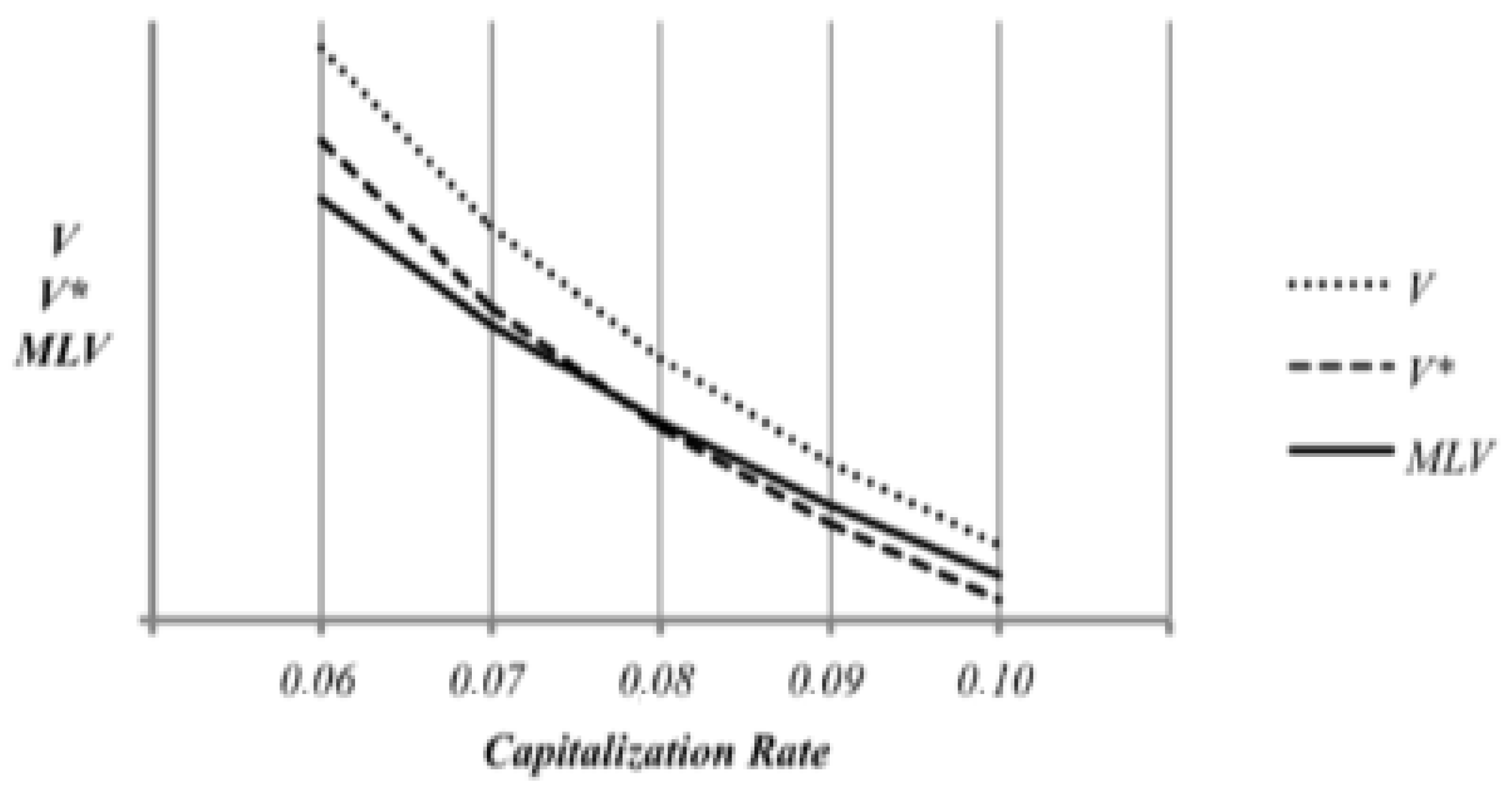
Formula (19) was examined using a particular situation (; ; ; ) and by changing one variable at a time (see Figure 2).
The market value, the bottom value, and the MLV decrease with the capitalization rate and tend to converge at higher rates. The bottom value is greater than MLV until a certain rate ( beyond which the bottom value is smaller than the MLV (see Figure 2).
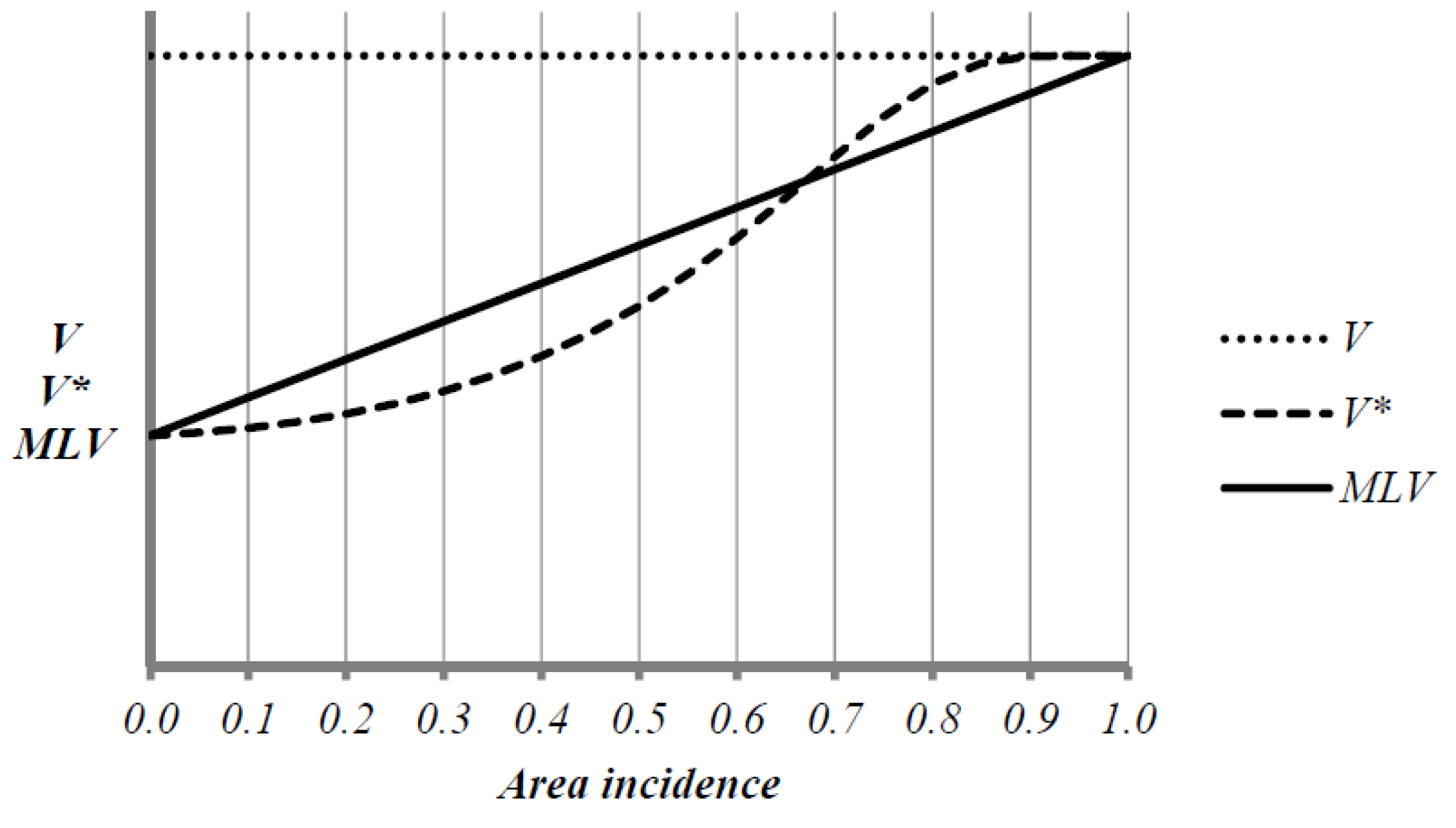
The bottom value and the MLV increase when the land incidence grows according to the market value, and then they tend to converge to the market value (; ; ) (see Figure 3). The MLV increases in a linear way; the bottom value is less than the MLV in the first section and is greater towards the end ( in Figure 3).
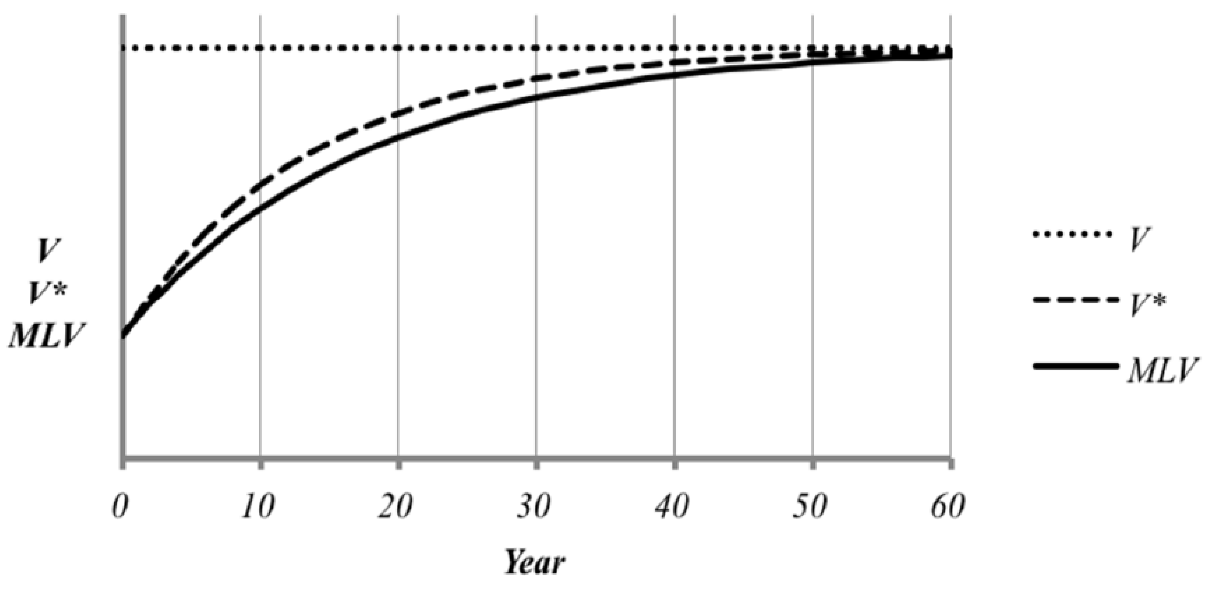
The bottom value and the MLV (; ; ; ; ) increase when the residual life increases, and they tend to converge with longer durations (see Figure 4). The bottom value is greater than the MLV for all durations.
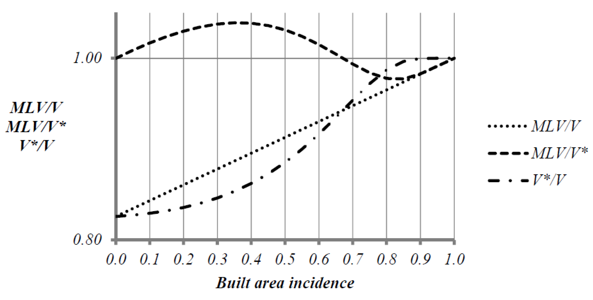
The ratio of the MLV to the bottom value referring to the incidence of the built area (22) and the incidence of income (23) (; ; ) is graphically rendered by Figure 5.
5. Conclusions
Generally, the MLV tends to underestimate the property market value due to its subdivision into two components: land and building. The determination of the building value through the income capitalization realistically considers the residual maturity of the building’s structure instead of an unlimited period, as happens for the land. The corresponding distribution of property income in these two parts is carried out according to the incidence of the land, typically estimated synthetically. To calculate land and building values, the capitalization rate is unique.
The elements of discretion in calculating the MLV are the percentages to be applied to the expenditure items in the determination of real estate net income, the measure of the land incidence rate, the capitalization rate (within a certain fixed interval), and the estimated time for the building demolition (within 30 years).
The ability to calculate the bottom value, given the capitalization and land incidence rates, allows taking a longer guarantee value, the latter up to the value of land incidence for which the bottom value is less than the MLV. Similarly, given the land incidence, it allows taking an MLV up to the value of the capitalization rate for which the MLV is less than the bottom value.
Author Contributions
Conceptualization, F.S., M.D.R., D.T., P.D.P. and F.P.D.G.; methodology, F.S., M.D.R., D.T., P.D.P. and F.P.D.G.; validation, F.S., M.D.R., D.T., P.D.P. and F.P.D.G.; formal analysis, F.S., M.D.R., D.T., P.D.P. and F.P.D.G.; investigation, F.S., M.D.R., D.T., P.D.P. and F.P.D.G.; data curation, F.S., M.D.R., D.T., P.D.P. and F.P.D.G.; writing—original draft preparation, F.S., M.D.R., D.T., P.D.P. and F.P.D.G.; writing—review and editing, F.S., M.D.R., D.T., P.D.P. and F.P.D.G. All authors have read and agreed to the published version of the manuscript.
Funding
This research received no external funding.
Institutional Review Board Statement
Not applicable.
Informed Consent Statement
Not applicable.
Data Availability Statement
Not applicable.
Conflicts of Interest
The authors declare no conflict of interest.
References
- Wild, T. Opinion of the European Banking Authority on Mortgage Lending Value (MLV); European Banking Authority: Paris, France, 2015. [Google Scholar]
- International Valuation Standard Council. International Valuation Application 2—Valuation for Lending Purposes; IVSC: London, UK, 2011. [Google Scholar]
- Ross, F.; Brachmann, R.; Renner, U.; Holzner, P. Ermittlung des Verkehrswertes von Grundstücken und des Wertesbaulicher Anlagen; OppermannVerlag: Rodenberg, Germany, 2005. [Google Scholar]
- Sommer, G.; Kröll, R. Lehrbuch zur Grundstückswertermittlung; LuchterhandVerlag: Wiesbaden, Germany, 2005. [Google Scholar]
- Rössler, R.; Langner, J. Schützung und Ermittlung von Grundstückswerten, 8th ed.; Luchterland Fachverlag: Munich, Germany, 2004; pp. S65–S78. [Google Scholar]
- Metzner, S. Einflussfaktoren auf Zwangsversteigerungserlöse bei Eigentumswohnungen. Grund. Grund. 2005, 4, S214–S220. [Google Scholar]
- Adolf, W. Der nachhaltige erzielbare Ertrag -ein veralteter Begriff? Grund. Grund. 2005, 4, Sl93–S197. [Google Scholar]
- Werth, A. VomVerkehrswertunabhängigeBeleihungswerteimBlcikfeld der Europäischen Union. Grund. Grund. 1998, 5, S257–S266. [Google Scholar]
- Rüchardt, K. Der Beleihungswert; Fritz Knapp Verlag: Frankfurt am Main, Germany, 2001. [Google Scholar]
- Stöcker, O.M. Realkredit und Pfandsicherheit—Der Beleihungswertim Bankenaufsichtsrecht; Fritz Knapp Verlag: Frankfurt am Main, Germany, 2004. [Google Scholar]
- Kierig, J. Zumneuen Pfandbriefgesetz und dem Entwurf der Beleihungswertermittlungsverordnung (BelWertV). Vortrag auf dem 14, Werterrnittlungsforurn, Jahreskongress. 2006. Available online: https://www.gesetze-im-internet.de/belwertv/BJNR117500006.html (accessed on 16 March 2022).
- Crosby, N.; French, N. Bank lending on business property—How do valuations aid the process? In Proceedings of the 19th ERES Conference, Athens, Greece, 22–25 June 1999. [Google Scholar]
- White, D.; Turner, J. Immobilienbewertung: Internationale Märkteverlangeninternationale Verfahren—BeleihungsobjektekönnenStichtagsbewertung ‘sprengen’. Immob.-Ztg. 1999. Available online: https://www.iz.de/unternehmen/news/-immobilienbewertu-internationa-maerk-verlang-internationaleverfahr-beleihungsobjek-koenn-stichtagsbewertu-spreng--marktentwicklungberuecksichtig--te--12183?crefresh=1 (accessed on 16 March 2022).
- Serret, A.; Trello, J. Reducing house prices, reducing mortgage risks. A methodology for measuring mortgage risk. In Proceedings of the ENHR Conference, Cambridge, UK, 2–6 July 2004. [Google Scholar]
- Adair, A.; Hutchison, N. The reporting of risk in real estate appraisal property risk scoring. J. Prop. Invest. Financ. 2005, 23, S254–S268. [Google Scholar] [CrossRef]
- Joslin, A. An investitgation into the expression of uncertainity in property valuation. J. Prop. Invest. Financ. 2005, 23, 269–285. [Google Scholar] [CrossRef]
- Crosby, N.; Hughes, C.; Murdoch, J. Influences on secured lending property valuations in the UK. In Proceedings of the ERES Conference, Milan, Italy, 2–5 June 2004. [Google Scholar]
- Bretten, J.; Wyatt, P. Variance in commercial property valuations for lending purposes: An empirical study. J. Prop. Invest. Financ. 2001, 19, S267–S282. [Google Scholar] [CrossRef]
- Ciuna, M.; De Ruggiero, M.; Salvo, F.; Simonotti, M. Measurements of rationality for a scientific approach to the market-oriented methods. J. Real Estate Lit. 2016, 24, 403–427. [Google Scholar]
- Bienert, S. Projektfinanzierung in der Immobilienwirtschajt; Deutscher Universitätsverlag: Wiesbaden, Germany, 2005. [Google Scholar]
- Pitschke, C. Die Finanzierung Gewerblicher Immobilien—Projektentwick Lungen unter Basel II; Immobilien Informations Verlag Rudolf Müller: Köln, Germany, 2004. [Google Scholar]
- Renaud, B. The 1985 to 1994 Global Real Estate Cycle—Its Causes and Consequence. In The World Bank—Financial Sector Development Department; Policy Research Working Paper No. 1452; The World Bank: Washington, DC, USA, 1995. [Google Scholar]
- Maier, K.M. Risiko Management Immobilienwesen—Leitfaden für Theorie und Praxis, 1st ed.; Fritz Knapp Verlag: Frankfurt am Main, Germany, 1999. [Google Scholar]
- Ropeter, S. lnvestitionsanalyse für Gewerbeimmobilien; Immobilien Informations Verlag Rudolf Müller: Köln, Germany, 1998. [Google Scholar]
- Wüstefeld, H. Risiko und Rendite von Immobilieninvestments, 1st ed.; Fritz Knapp Verlag: Frankfurt am Main, Germany, 2000; pp. 51–228. [Google Scholar]
- Pfnür, A.; Armonat, S. Immobilien Kapitalanlage Institutioneller Investoren: Risikomanagement und Portfolioplanung; Ergebnisbericht zur Empirischen Untersuchung, Universitat Hamburg/Eversmann & Partner—Corporate Real Estate: Hamburg, Germany, 2001. [Google Scholar]
- PWC. VI—European house prices. In European Economie Outlook; Pricewaterhouse Coopers: London, UK, 2004; pp. S25–S30. [Google Scholar]
- Milleker, D.F. International Housing Markets: How Diffìcult a Retum to Normal? Working Paper No. 37; Allianz Group: Frankfurt am Main, Germany, 2005. [Google Scholar]
- Tsatsaronis, K. What drives housing price dynamics: Cross-country evidence. BIS Quarterly Review, 1 March 2004. [Google Scholar]
- Jorion, P. Value at Risk, 2nd ed.; McGraw-Hill: New York, NY, USA, 2000. [Google Scholar]
- Poppensieker, T. Skategisches Risikomanagement. In Deutschengroβbanken; Deutscher Universitätsverlag: Wiesbaden, Germany, 1997. [Google Scholar]
- French, N.; Gabrielli, L. Uncertainty and feasibility studies: An Italian case study. J. Prop. Invest. Financ. 2006, 24, 49–67. [Google Scholar] [CrossRef] [Green Version]
- Benevenuti, A. Financial and estimating indicators for assessment of mortgage lending value. Aestimum 2012, 621–628. [Google Scholar] [CrossRef]
- Tajani, F.; Morano, P. An empirical-deductive model for the assessment of the mortgage lending value of properties as securities for credit exposures. J. Eur. Real Estate Res. 2018, 11, 44–70. [Google Scholar] [CrossRef]
- Süchting, P. Theorie und Politik der Unternehmensfinanzierung, 6th ed.; Betriebswirtschaftlicher Verlag Dr. Th. Gabler GmbH: Wiesbaden, Germany, 1995. [Google Scholar]
- Rode, D. Grundzlige des Hypothekarkredits. In Handbuch des Hypothekarkredits—lmmobilienfinanzierung in Deutschland unf Europa, 3rd ed.; Konrad, R., Ed.; Fritz Knapp Verlag GmbH: Frankfurt am Main, Germany, 1993; pp. S23–S101. [Google Scholar]
- Rüchardt, K. Bewertung und Krediturtei. In Handbuch des Hypothekarkredits—lmmobilienfinanzierung in Deutschland und Europa; Konrad, R., Ed.; Fritz Knapp Verlag GmbH: Frankfurt am Main, Germany, 1993; pp. 143–261. [Google Scholar]
- Paschedag, H. Darlehens∙und Hypothekenfìnanzierung. In Handbuchlmmobilien-Banking—Vor der Traditionellenlmmobilien Finanzierungzumlmmobilien-Investmentbanking; Schulte, K.-W., Achleitner, A.K., Knobloch, B., Eds.; Immobilien Informations Verlag Rudolf Müller GmbH & Co. KG: Koln, Germany, 2002; pp. 69–87. [Google Scholar]
- Steffan, F.; Scholz, H. Finanzierungsanfragen, Objekte und Partner des Hypothekarkredits. In Handbuch des Hypothekarkredits: Lmmobilienfinanzierung in Deutschland und Europa, 3rd ed.; Konrad, R., Ed.; Fritz Knapp Verlag GmbH: Frankfurt am Mam, Germany, 1993; pp. 101–143. [Google Scholar]
- Low, S.; Sebag-Montefiore, M.; Dübel, A. Study on the Financial Integration of European Mortgage Markets; working paper; Mercer Oliver Wyman: London, UK, 2003. [Google Scholar]
- Gondring, H.; Lorenz, T. Basel II—Auswirkungen auf die lmmobilienwirtschaft; Akademie der Immobilienwirtschaft (ADI): Stuttgart, Germany, 2001. [Google Scholar]
- Bienert, S.; Brunauer, W. The mortgage lending value: Prospects for development within Europe. J. Prop. Invest. Financ. 2007, 25, 542–578. [Google Scholar] [CrossRef]
- European Parliament and Council of The European Union Industry. Directive 98/32/Ec; European Union: Luxembourg, 1998. [Google Scholar]
- TEGoVA. European Valuation Standards, 9th ed.; TEGoVA: Brussels, Belgium, 2020. [Google Scholar]
- Regulation (EU) of the European Parliament and of the Council of 26 June 2013 on Prudential Requirements for Credit Institutions and Investment Firms and Amending, 575. 2013. Available online: https://eur-lex.europa.eu/legal-content/EN/TXT/?uri=celex%3A32013R0575 (accessed on 16 March 2022).
- Ciuna, M.; D’Amato, M.; Salvo, F. Appraising building area’s index numbers using Repeat Value Model. A case study in Paternò (CT), in Dynamics of Land Values and Agricultural Policies. In Proceedings of the MediaMond International Proceedings, Bologna, Italy, 9–13 May 2013; pp. 63–71. [Google Scholar]
- Ciuna, M.; D’Amato, M.; Salvo, F. The appraisal smoothing in the real estate indices, in Dynamics of Land Values and Agricultural Policies. In Proceedings of the MediaMond International Proceedings, Bologna, Italy, 9–13 May 2013; pp. 73–83. [Google Scholar]
- Salvo, F.; Ciuna, M.; De Ruggiero, M. Property prices index numbers and derived indices. Prop. Manag. 2014, 32, 139–153. [Google Scholar] [CrossRef]
- Del Giudice, V.; De Paola, P.; Forte, F. The appraisal of office towers in bilateral monopoly’s market: Evidence from application of Newton’s physical laws to the Directional Centre of Naples. Int. J. Appl. Eng. Res. 2016, 11, 9455–9459. [Google Scholar]
- Del Giudice, V.; De Paola, P. Undivided real estate shares: Appraisal and interactions with capital markets. Appl. Mech. Mater. 2014, 584–586, 2522–2527. [Google Scholar] [CrossRef]
- De Ruggiero, M.; Forestiero, G.; Manganelli, B.; Salvo, F. Buildings Energy Performance in a Market Comparison Approach. Buildings 2017, 7, 16. [Google Scholar] [CrossRef]
- Acampa, G.; Forte, F.; De Paola, P.B.I.M. Models and evaluations. In Green Energy and Technology; Springer: Berlin/Heidelberg, Germany, 2020; pp. 351–363. [Google Scholar]
- Del Giudice, V.; Massimo, D.E.; De Paola, P.; Forte, F.; Musolino, M.; Malerba, A. Post Carbon City and Real Estate Market: Testing the Dataset of Reggio Calabria Market Using Spline Smoothing Semiparametric Method. In New Metropolitan Perspective; Springer International Publishing: Cham, Switzerland, 2019; ISBN 978-3-319-92098-6. [Google Scholar]
- Engle, R.F. Autoregressive conditional heteroscedasticity with estimates of variance of United Kingdom inflation. Econometrica 1982, 50, 987–1008. [Google Scholar] [CrossRef]
- Sornette, D.; Johansen, A.; Bouchaud, J.P. Stock market crashes, precursors and replicas. J. Phys. I 1996, 6, 167–175. [Google Scholar] [CrossRef] [Green Version]
- Sornette, D.; Johansen, A. Large financial crashes. Physica A 1997, 245, 411–422. [Google Scholar] [CrossRef] [Green Version]
- Yang, D.; Zhang, Q. Drift-independent volatility estimation based on high, low, open and close prices. J. Bus. 2000, 73, 477–491. [Google Scholar] [CrossRef] [Green Version]
- Andersen, T.G.; Bollerslev, T.; Diebold, F.X.; Labys, P. Modeling and forecasting realized volatility. Econometrica 2003, 71, 579–625. [Google Scholar] [CrossRef] [Green Version]
- Cajueiro, D.O.; Tabak, B.M. Testing for time-varying long-range dependence in volatility for emerging markets. Physica A 2005, 346, 577–588. [Google Scholar] [CrossRef]
- Wang, F.Z.; Yamasaki, K.; Havlin, S.; Stanley, H.E. Multifactor analysis of multiscaling in volatility return intervals. Phys. Rev. E 2009, 79, 16103. [Google Scholar] [CrossRef] [PubMed] [Green Version]
Figure 1.
Transitory cash-flows.

Figure 2.
Relationship between V, V*, and MLV and the capitalization rate.

Figure 3.
Relationship between V, V* and MLV and the area incidence.

Figure 4.
Relationship between V, V*, and MLV and the years.

Figure 5.
Relationship between MLV/V, MLV/V*, and V*/V and the built area incidence.

Publisher’s Note: MDPI stays neutral with regard to jurisdictional claims in published maps and institutional affiliations. |
© 2022 by the authors. Licensee MDPI, Basel, Switzerland. This article is an open access article distributed under the terms and conditions of the Creative Commons Attribution (CC BY) license (https://creativecommons.org/licenses/by/4.0/).
Share and Cite
MDPI and ACS Style
Salvo, F.; De Ruggiero, M.; Tavano, D.; De Paola, P.; Del Giudice, F.P. Analytical Implications of Mortgage Lending Value and Bottom Value. Buildings 2022, 12, 799. https://doi.org/10.3390/buildings12060799
AMA Style
Salvo F, De Ruggiero M, Tavano D, De Paola P, Del Giudice FP. Analytical Implications of Mortgage Lending Value and Bottom Value. Buildings. 2022; 12(6):799. https://doi.org/10.3390/buildings12060799
Chicago/Turabian StyleSalvo, Francesca, Manuela De Ruggiero, Daniela Tavano, Pierfrancesco De Paola, and Francesco Paolo Del Giudice. 2022. "Analytical Implications of Mortgage Lending Value and Bottom Value" Buildings 12, no. 6: 799. https://doi.org/10.3390/buildings12060799
Note that from the first issue of 2016, this journal uses article numbers instead of page numbers. See further details here.