
Bipedal Robot Gait Generation Using Bessel Interpolation

1
Department of Mechanical and Energy Engineering, Southern University of Science and Technology, Shenzhen 518055, China
2
Health Management System Engineering Center, School of Public Health, Hangzhou Normal University, Hangzhou 311121, China
3
Institute of Oceanographic Instrumentation, Qilu University of Technology (Shandong Academy of Sciences), Qingdao 266075, China
*
Authors to whom correspondence should be addressed.
Biomimetics 2024, 9(4), 201; https://doi.org/10.3390/biomimetics9040201
Submission received: 3 January 2024
/
Revised: 23 March 2024
/
Accepted: 25 March 2024
/
Published: 28 March 2024
(This article belongs to the Section Bioinspired Sensorics, Information Processing and Control)
Abstract
:This paper introduces a novel approach to bipedal robot gait generation by proposing a higher-order form through the parameter equation of first-order Bessel interpolation. The trajectory planning for the bipedal robot, specifically for stepping up or down stairs, is established based on a three-dimensional interpolation equation. The experimental prototype, Roban, is utilized for the study, and the structural sketch of a single leg is presented. The inverse kinematics expression for the leg is derived using kinematic methods. Employing a position control method, the angle information is transmitted to the robot’s joints, enabling the completion of both downstairs simulation experiments and physical experiments with the Roban prototype. The analysis of the experimental process reveals a noticeable phenomenon of hip and ankle joint tilting in the robot. This observation suggests that low-cost bipedal robots driven by servo motors exhibit low stiffness characteristics in their joints.
1. Introduction
Bipedal robots, designed to emulate human walking, possess distinctive features, such as a high center of gravity and a discrete distribution of landing points. This makes them a focal point of research in the robotics field. In China, the current robot industry is experiencing rapid growth, and biped robots are increasingly integral to the human-machine society, owing to their humanoid motion capabilities. Particularly, at the consumer level, bipedal robots often utilize servo motors due to their cost-effectiveness and ease of integration. However, the prevalent use of servo motors in bipedal robots introduces challenges associated with low joint stiffness. This results in significant joint errors when executing simple task actions through open-loop control. This paper addresses these challenges by employing the Bessel interpolation method to generate gait trajectories for robots stepping up or down stairs. This approach enhances the robot’s motion performance, enabling it to navigate uneven ground and execute tasks with improved precision and stability.
The evolution of bipedal robots has spurred heightened interest in the research of their gait and footprint planning. Currently, two predominant methods are employed for generating gait trajectories in bipedal robots. One approach involves mimicking human neural reflexes to derive the robot’s gait trajectories. The other mainstream method relies on classical dynamics, wherein gait trajectories are generated by constructing dynamic models or utilizing mathematical interpolation methods. This section focuses on introducing the research content pertaining to the generation of gait trajectories in bipedal robots using the latter, i.e., the classical dynamics-based method. For example, Kajita proposed a linear inverted pendulum (LIPM) model for complex road surfaces in 1991, and its simulation experiments showed that the walking performance of the control method on specific rough terrain is comparable to that of the robot walking on horizontal ground [1]. Subsequently, Kajita combined the linear inverted pendulum model with the ZMP method to apply to a bipedal robot. This method requires the robot to maintain a constant center of mass (COM), and therefore the ASIMO robot bends its knees to move forward [2]. Subsequently, some scholars have improved the algorithm and proposed algorithms such as the Divergent Component of Motion (DCM) algorithm [3], Spatial Quantized Dynamics (SQD) algorithm [4,5,6], the Virtual Mass Ellipsoid Inverted Pendulum (VIP) algorithm [7], etc. Nishiwaki introduced an online method in 2002 that achieves a smooth connection between the subsequent centroid trajectory and the current trajectory by solving the difference equation [8]. Harada used analytical methods in 2004 to smoothly connect COG trajectories to existing trajectories, allowing the robot’s footsteps to change quickly and smoothly [9]. Morisawa improved this method in 2007, allowing robots to adjust their footsteps at any time [10]. In 2014, Samadi also explored the use of the gravity compensated inverted pendulum mode (GCIPM) pattern generation method to generate walking trajectories while ensuring the robot supported the foot movement’s ZMP during stepping [11]. In 2014, Garton detailed the use of a linear inverted pendulum (LIPM) to plan walking trajectories, enabling robots to steadily move forward, stop and restore their direction of motion. He pointed out that the use of a fixed step cycle duration reduces the complexity of mathematics and the amount of computation, thus completing the simplified process of motion planning for the bipedal robot [12]. Imanishi proposed a new bipedal gait control in 2018, which does not rely on time-defined trajectories. The motion rate of the center of mass relative to ZMP is expressed as the gradient of potential. In each step, the potential monotonically decreases from positive to negative, while the positive potential encourages lifting and the negative potential reminds the robot to touch the ground, making the robot’s feet stable and alternating [13]. There are also some other methods for generating gait models, such as using the Hybrid Zero Dynamics (HZD) model [14,15,16]. In addition to model-based methods, spline interpolation can also be used for gait generation, including methods such as cubic and quintic splines [17,18,19,20,21,22]. After gait generation, the Whole Body Control (WBC) and the Model Predictive Control (MPC) methods can be used for robot control [23,24,25,26,27,28,29,30,31].
This paper utilizes the Bessel interpolation method for planning the Roban robot’s gait trajectory. The joint angles are determined through the inverse solution of robot kinematics, and motion execution employs a position control method. The study encompasses both simulation and prototype experiments, with the Roban robot navigating stairs in the V-REP simulation software and a physical prototype experiment simultaneously. The Roban robot, with 12 degrees of freedom in its legs, was provided by China Leju Company. The second section details the establishment of Bessel interpolation, the third section outlines the inverse kinematics solution for the Roban robot, and the fourth section describes the experimental process of the bipedal robot stepping downstairs using Bessel interpolation. The fifth section concludes, a summary of the findings and suggestions for future research studies.
2. Inverse Kinematics of Roban Robots
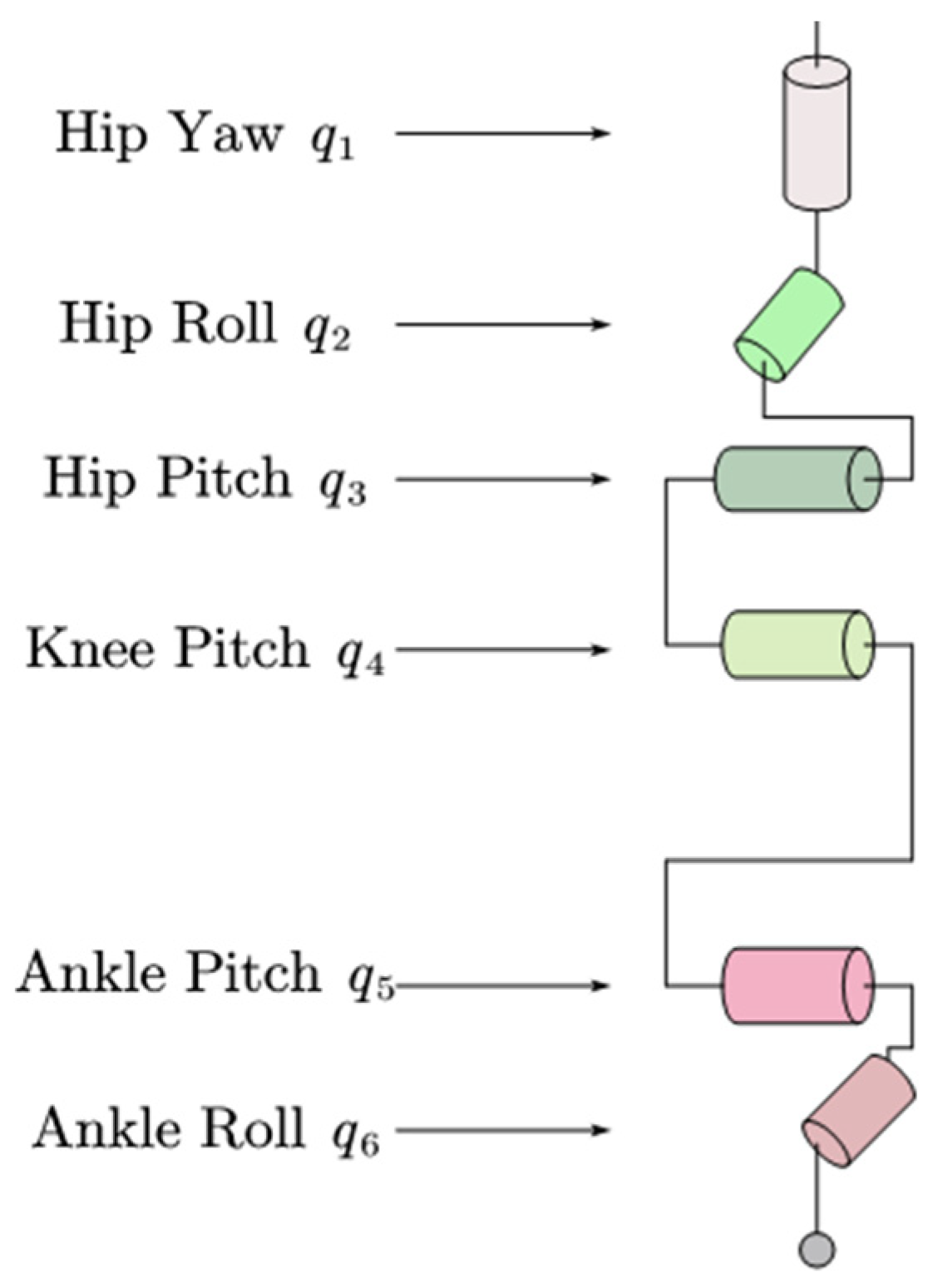
Solving the inverse kinematics of a robot involves calculating the angles or movements of each joint based on the robot’s base posture and end configuration. Given that the upper body of the Roban robot functions as a floating base, inverse kinematics calculations are applied to its lower limbs. During low-speed operations, open-loop control is utilized for task execution, and the robot’s joint angle information is derived from its kinematic model. Subsequently, the bipedal robot transmits this angle information to the servo driver through position control, facilitating the execution of the specified task. To obtain the joint angle information for the Roban robot, its legs are modeled using inverse kinematics, as illustrated in Figure 1, depicting the distribution of joint degrees of freedom in a single leg of the Roban robot.
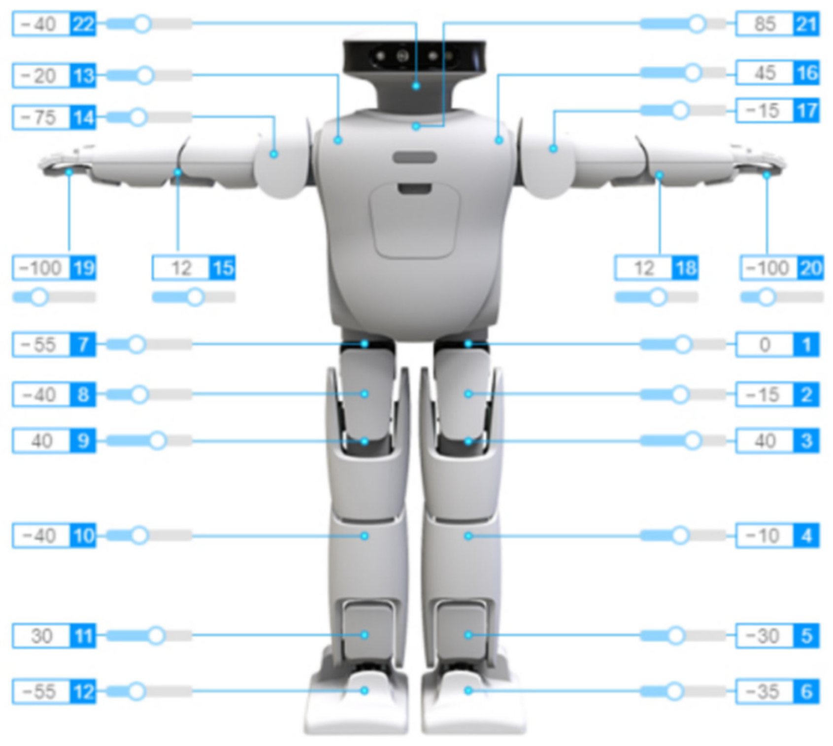
The Roban robot has six degrees of freedom in a single leg, and each joint is equipped with a steering gear. The hip joint is composed of hip yaw, hip roll and hip pitch. The knee joint consists of knee pitch, and the ankle joint consists of an ankle roll and ankle pitch. From top to bottom, the label and angle information of the joint servo are to . The joint servo rotates with the vertical line of the ground as its axis; and are rotated in the forward direction of the robot; , , are rotated with the lateral axis of the robot. The base coordinate system of the robot is placed on the hip joint. From the perspective of the robot in the forward direction, the forward direction is the X-axis, leftward is the Y-axis, and vertical upward is the z-axis. Therefore, the roll angle is rotated around the X-axis, the pitch angle rotates around the Y-axis, and the yaw angle is rotated around the z-axis. This roll-pitch-yaw way of describing the robot pose is known as the Euler angle method.
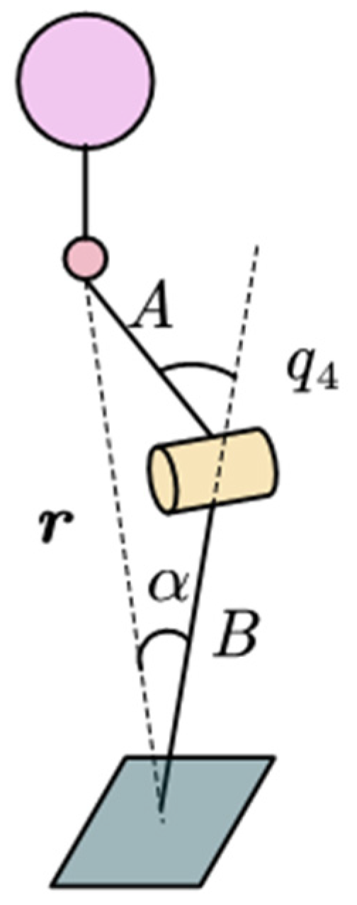
When solving the inverse kinematics of the Roban robot, it is first simplified to the triangle shown in Figure 2. is the thigh length of the Roban robot; is the leg length of the robot; is the vector from hip to ankle, and its length is represented by the modulo length .
The poses of the robot’s torso and feet are (, ) and (, ), with the distance from the torso to the hip joint denoted by , where is the position vector and is the rotation matrix of each joint’s coordinate system, set to E and parallel to the world coordinate system, which is defined on the joint cross axis. According to the forward kinematics of the robot, the hip joint position is calculated as follows:
The r is defined as follows:
Then the length of C is as follows:
Given the length of A, B and C, q4 can be written as
From the law of cosine, the angle α is
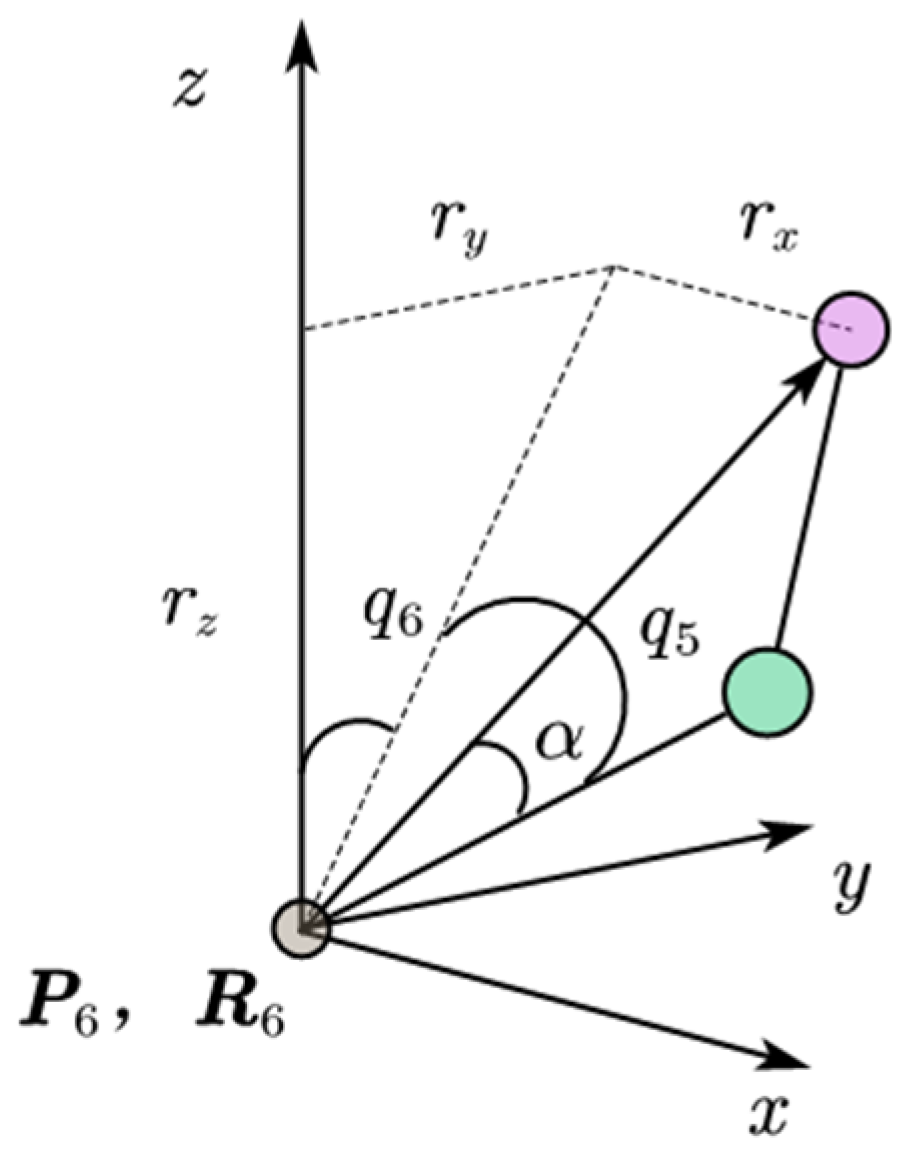
Figure 3 shows the coordinate system of the Roban robot’s single leg ankle joint. The angles of the ankle joint, denoted by and , can be represented as follows:
where atan2 is the inverse tangent function.
According to , , of the robot, , , are solved. According to the forward kinematics of the robot, the posture of the foot sole can be obtained as follows:
The rotation matrix of the robot is an orthogonal matrix, and its property is
From Equation (9), Equation (8) can be rewritten as
The joint of the Roban robot rotates around roll, pitch and yaw, and the corresponding rotation matrix is the following:
Given the angle and rotation axis of the joint steering gear of the Roban robot, denoted by , and , the right side of Equation (10) is a definite matrix, expressed as
From Equation (11) to Equation (13), the expression of , and can be obtained as follows:
Thus,
Among them, by analogy with and , the remaining identity meanings can be obtained. Finally, the expressions of , and can be obtained as follows:
At this point, the inverse kinematics expression of the Roban robot is solved.
3. Bessel Interpolation Method
Discontinuous gait trajectories in robots can lead to infinite acceleration and rigid impacts, posing a risk of damage due to the resulting torque on joint actuators. To avoid such issues, bipedal robots must adhere to smooth trajectories during walking tasks. Currently, gait modeling based on 3D linear inverted pendulum or Zero Moment Point (ZMP) methods is prevalent. These methods are mutually inverse in terms of input and output. When navigating designated slope step ground, Z-direction trajectory interpolation is necessary for bipedal robots using these approaches. Alternatively, bipedal robots can employ the Virtual Mass Ellipsoid Inverted Pendulum (VIP) method to handle non-planar problems, typically requiring computer-based solutions. However, for low-cost robot prototypes engaged in low-speed motion, the reliance on computer performance is minimized. Thus, this section adopts the Bessel interpolation method for generating the gait trajectory of the bipedal robot, focusing on the generation process in detail.
3.1. Use and Characteristics of Bezier Curve
Bezier curve was originally an application curve of two-dimensional figure. Its mathematical expression was originally derived from Bernstein polynomials, which proved that continuous function within the [a, b] interval can be approximated by polynomials, and the approximated functions have strong convergence. For a continuous function, multiple Bernstein polynomials can be selected. When the order of Bernstein polynomials approaches infinity, the polynomial will converge to the original function. Later, French mathematician Casteljau graphically processed the polynomial and proposed a corresponding numerical solution algorithm to generate a fitted two-dimensional graphical curve. Pierre Bezier, a French engineer, used this method to complete the industrial design of the auxiliary car body and spread it widely. Therefore, this method is called the Bessel interpolation method. At present, this method can not only fit two-dimensional curves but also complete curve fitting in space. It includes three types of sampling points, namely: the starting point, the control point and the ending point. The Bezier curve can be changed by adjusting the control points, and the curvature of the Bezier curve can be adjusted. The method of changing the curvature of the Bezier curve by adjusting the control points is very important for the gait adjustment of subsequent robots. The Bessel interpolation method is now used to complete the design of robots’ downstairs gait trajectory.
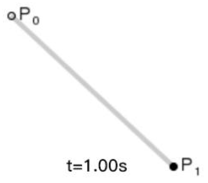
The Bezier curve can be constructed by setting sampling points, which include the starting point, the ending point and the control point. By adjusting the number of control points, the degree of the Bezier curve can be adjusted. For example, a first-order Bezier curve is composed of two points, 0 control points, and the fitted Bezier curve is a first-order straight line. Its expression is as follows:
where P0 and P1 are the start and end points of the Bezier curve, and t is the parameter, whose curves are shown in Figure 4.
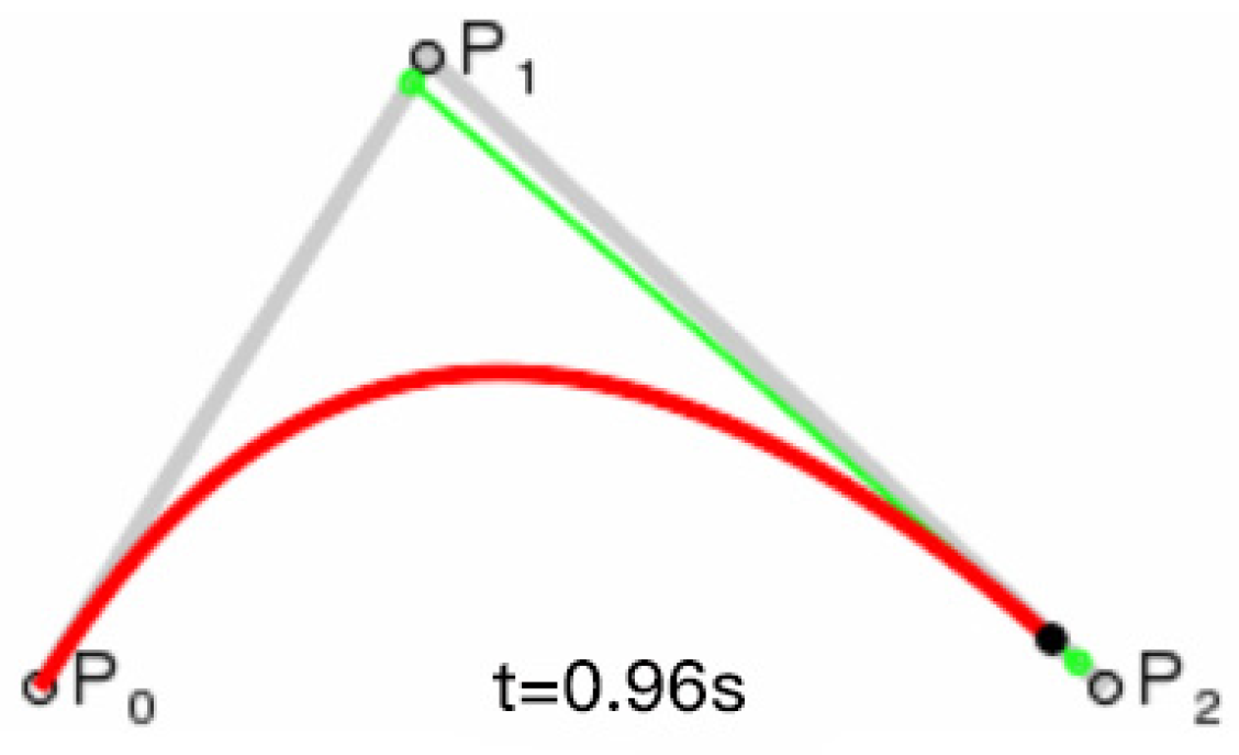
When the control point is 1, the fitted Bezier curve is a second-order curve, and its expression is as follows:
The and are the starting and ending points of the Bezier curve, and is the control point. The final expression is a conic, as shown in Figure 5. The Bezier curves for the remaining orders are followed in the same way.
The Bezier curve exhibits three key characteristics: it passes through both the starting and ending points and is tangent to the feature line at both ends. The control point influences the curvature of the Bezier curve by pulling the fitted curve toward the current control point, providing convenient adjustment of the curve’s radian. Planar control points play a crucial role in shaping the curve, as altering their coordinates directly impacts the fitted Bezier curve’s form. The Bezier curve lies within the convex hull of the feature polygon, offering a smoother representation compared to the polygon.
Widely employed in computer graphics, the Bezier curve is created and edited with simple starting points, ending points and control points. Adjusting the starting and ending points alters the position of the Bezier curve in the world coordinate system, while changing the control points influences the curvature to meet the requirements of bipedal robots. For instance, when modifying the Bezier curve trajectory of a bipedal robot’s swing leg, it allows for the adjustment of the swing leg’s stability during the swinging process. Due to their capacity for easy adjustment of sample points, Bezier curves serve as an ideal tool for graphic editing and creation, being utilized by engineers, academics and other professionals.
3.2. Higher Order Bezier Curve Fitting Method
The order of the Bezier curve varies with the number of control points. As mentioned in the previous section, when the Bezier curve has zero control points, the Bezier curve is a first-order line segment. When the Bezier curve has one control point, the Bezier curve is a second-order quadratic curve and so on. The mathematical formulas of the first and second order curves are given in the above subsections. In the following, the expression of the second order and the formula of the higher order Bezier curve are derived from the first order formula.
The first-order Bezier curve has two points, namely the points and , and its parametric equation can be expressed as Equation (20).
The quadratic Bezier curve has three points, respectively, , and , where and , respectively, are fixed points on a line P0P1 and P1P2. According to the first-order Bezier curve, the parametric equations of and are as follows:
By fitting the parametric equations of and according to the first-order equation, we can get the following:
For the expression of the Bezier curve of higher order, suppose that is the coefficient of the kth point of the Bezier curve of order. In the , by utilizing the second order Bessel method based on Pk in , will transition to . In the function Bn(t), in the presence of a new parameter, , it can be expressed as .
The following condition needs to exist:
to prove the following equation:
When , Equation (27) conforms to the law of Equation (26), and the result still holds. Thus, the induction hypothesis holds and the Equation (28) for Bezier curves of any order n is obtained. Using this formula, the gait trajectory of a robot based on the Bezier method can be generated.
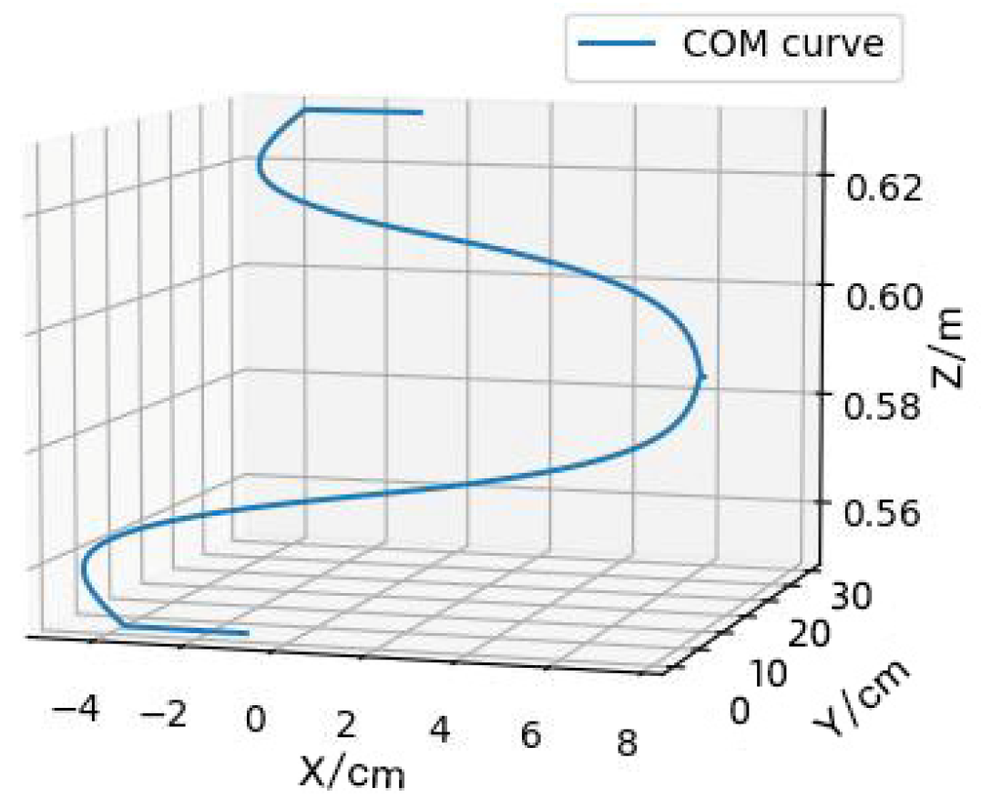
According to this method and based on specific parameters, such as the robot’s centroid position, step height, step length, foot length and so on, the Bezier curve of the robot centroid is planned and generated, as shown in Figure 6.
4. Experiments
The Roban robot underwent stair simulation experiments using Virtual Robot Experimentation Platform (V-REP) software, alongside completing a physical prototype experiment of stepping downstairs. The experimental results validate the efficacy of the Bessel interpolation-based gait generation method and shed light on the specific motion characteristics of low-cost bipedal robots under open-loop control. These findings enhance our understanding of the practicality of the proposed approach in real-world scenarios.
4.1. The Bipedal Roban Robot
This experimental platform utilizes the bipedal robot prototype, Roban, provided by Leju (Shenzhen) Robot Technology Co., Ltd., Shenzhen, China. The prototype serves as an AI display and application platform, based on ROS, for higher education institutions, research institutes and other scientific research organizations. It boasts characteristics such as open-source architecture and scalability. Equipped with a depth camera, a built-in V-SLAM vision algorithm and compatibility with platforms such as UCF and Microsoft, it excels in intelligent operations such as speech recognition, SLAM-based indoor navigation mapping, walking along curves and executing movements on slopes and stairs. Leju offers a comprehensive set of educational programs for artificial intelligence talents, covering topics ranging from programming and robot motion control to computer vision. These programs are suitable for independent learning by students majoring in mechanical, computer, automation and related disciplines. Figure 7 illustrates the Roban robot, providing details on the distribution of its degrees of freedom and the zero offset for each joint.
The remaining content is shown in Table 1.
4.2. Simulation Experiment
The Bessel interpolation method falls under the category of static gait trajectory generation. When the robot employs position control, the Bessel interpolation method is effective in generating the low-speed gait required for descending stairs. Considering the hardware parameters of the Roban robot, the chosen steps for the experiment are 50 cm in length, 15 cm in width and 4 cm in height.
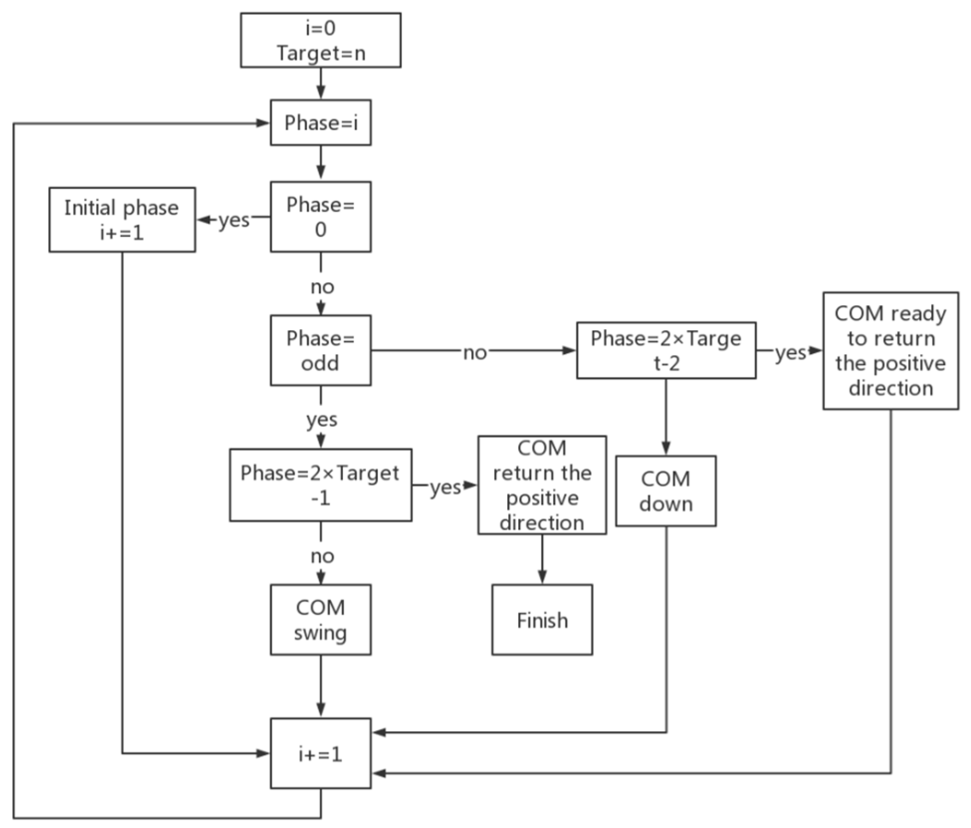
The stair-stepping simulation experiment is conducted in V-REP after establishing the step simulation environment. Initialization tasks, including ROS and joint variable initialization, are undertaken. ROS-based publisher and subscriber are defined to facilitate information exchange. The robot executes motion actions based on Bezier curves using position control. Starting from the initial standing position, the robot smoothly navigates the stair descent process, employing Bezier interpolation to generate its trajectory in each phase of the experiment. The phases include the following: phase = 0, phase = odd, phase = even, phase = 2 × Target (the number of Target stairs)-2, phase = 2 × Target-1. The complete process of going down the stairs can be summarized by the flow chart shown in Figure 8.
Phase = 0 is the initial descent phase of the robot on the stairs. During this phase, the robot completes the left swing of the hip joint, so that its center of mass is closer to the left, and initiates the swing of its right leg.
Phase = odd is the swing phase of the robot’s center of mass during the process of stepping downstairs; for example, when phase = 1, the robot has just completed the descent of one step, and its center of mass is on the left. If the robot lifts its left foot at this time, the robot will fall down. Therefore, the center of mass of the robot is set to move to the right, and this stage is the center of mass translation stage.
In even phases (phase = even), the center of mass of the robot descends the stairs during the process of going down the stairs. For example, when phase = 2, the robot completes the change of the center of mass. The robot lifts its left leg and completes the descent process of two steps; this phase is the centroid dropping phase of the robot.
Phase = 2 × Target-2 is the phase when the robot is ready to return to the positive direction; for example, the robot’s target falls to the third step, that is, Target = 3. When the phase = 4, the swing leg of the robot completes the descent of one step. Both of its feet should finally land on the same step, marking this phase as the foot recovery phase of the robot.
Phase = 2 × Target-1 is the phase when the robot returns to the upright position; for example, at phase = 5, the robot’s feet return to the upright position because the mass is centered on the left. To make the robot stand completely straight, the center of mass of the robot is translated to the right. This stage is the center of mass of the robot back to the positive stage.
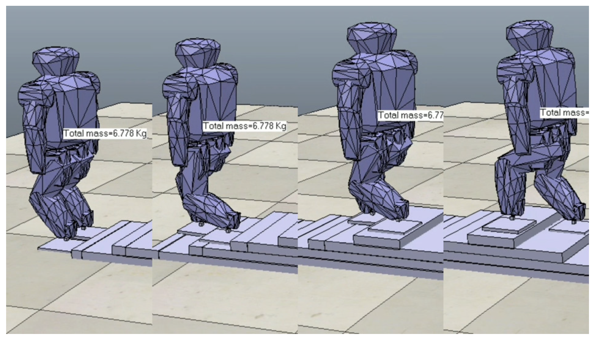
According to the above design process and step parameters, the descent trajectory of a bipedal robot based on the Bezier curve is designed. The Roban robot generates the position information transmitted to the joint servo through its inverse kinematics expression, and it can successfully perform the downstairs task on the V-REP simulation platform, based on ROS, as shown in Figure 9.
4.3. Prototype Experiment
When the simulation code is fully utilized in the prototype’s downstairs experiment, the results prove less than ideal. Through adjustments to the Bezier curve’s curvature and the time period for the servo to accept position commands, the Roban prototype achieves successful stair-stepping. Influential input parameters for Bezier curvature include the robot’s centroid position, step height, step length and foot length. Despite these parameters being determined in the physical world, the robot’s inherent errors necessitate further adjustments to execute the stair-stepping task based on Bezier curves. Several considerations are essential during this adjustment phase:
- (1)
- Parameters for adjusting the robot’s position:
Adapting the robot’s center of mass prevents forward or backward falls during leg swings.
Altering the trajectory of the robot’s legs addresses issues with the foot falling prematurely before lifting off the steps.
Adjusting the control point of the trajectory affects the position and swing inertia of the robot’s swing foot.
Continuous trajectory adjustments are crucial to prevent robot shaking or instability during stair descent.
- (2)
- Adjustment of the robot’s time cycle parameters:
Given that this static gait method suits slow descents, an overly fast overall speed introduces significant inertia during leg swings and center of mass translation.
Increasing the running time of the overall robot reduces inertia, preventing forward or backward falls.
- (3)
- Parameters for adjusting the robot’s step height:
Similar to adapting the trajectory of the robot’s legs, this parameter prevents the robot’s feet from falling prematurely before lifting off the step plane.
- (4)
- Parameters for adjusting the robot’s step length and foot length:
To address the accumulated errors observed during the stair descent process, adjusting these parameters helps maintain the intended distance for each step.
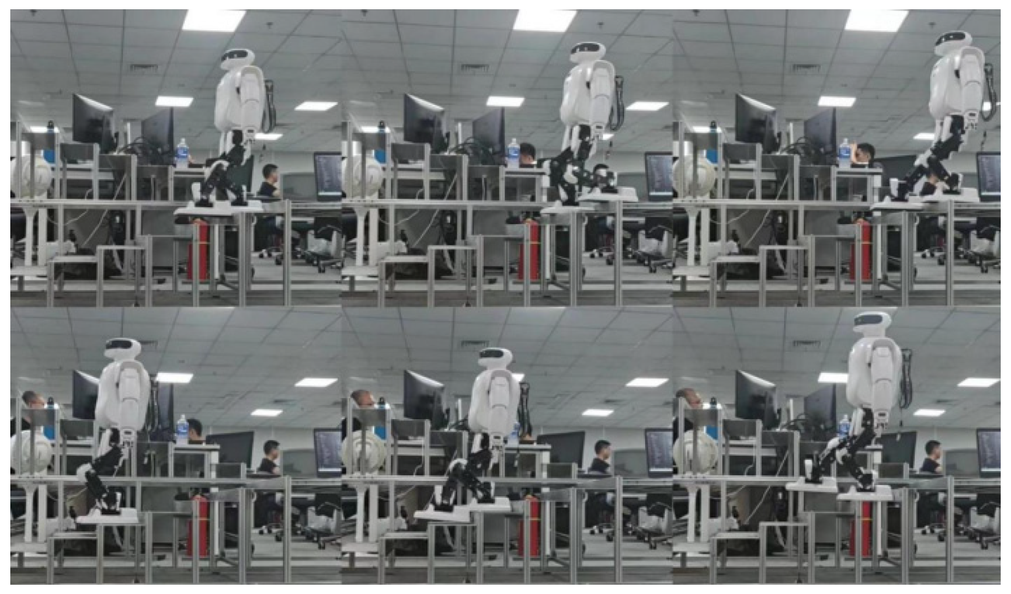
Following the meticulous adjustment of these parameters, the Roban robot successfully executes the stair-stepping process in the real world, as illustrated in Figure 10.
Examining the Roban robot’s stair descent process in the figure above reveals significant errors, including jitter, hip joint tilt, backward tilt and misalignment of the ankle joint with the step surface. These issues stem not only from limitations in the static gait method but also from various errors within the Roban prototype itself, such as servo installation discrepancies, manufacturing inaccuracies, and the inherent low-bending stiffness of gears. These factors collectively contribute to insufficient joint stiffness in both the hip and ankle joints of the bipedal robot. Addressing these challenges requires ongoing refinement in both gait generation methods and mechanical components to enhance overall performance and stability during complex tasks like stair descent.
5. Conclusions
This paper introduces the Bezier interpolation method for generating the gait trajectory of the Roban robot during stair descent. The inverse kinematics expression of the robot is solved, and the Bezier gait curve is successfully applied to both the staircase simulation and prototype experiments using position control. The analysis of the experiment video reveals that the Roban robot exhibits jitter, hip joint tilt, backward tilt and an ankle joint misalignment with the step surface. These observations are attributed to the low joint stiffness of the Roban robot. Despite these challenges, this research lays the groundwork for improving the motion performance of low-cost bipedal robots, offering valuable insights for future development.
Author Contributions
Conceptualization, Z.W.; software, Z.W. and Q.L.; validation, Z.W.; formal analysis, Q.L. and D.Z.; resources, Q.L. and W.K.; data curation, L.K. and D.Z.; writing—original draft, Q.L.; writing—review and editing, D.L.; visualization, L.K. and D.Z.; supervision, W.K.; project administration, L.K., W.K. and D.L.; funding acquisition, W.K. and D.L. All authors have read and agreed to the published version of the manuscript.
Funding
This research is sponsored by the following funds: (1) Public welfare technology research project of Zhejiang Provinces Science Foundation in China. The effect model construction and 3D visualization of auricular point pivot regulation of brain neural (No. LGF20F020009). (2) Key R&D Program of Zhejiang Province. Research on Intelligent Service Technology and Equipment of Health and Elderly Care—support the research and application development of medical nursing care robot and elderly care service system of Internet hospitals (No. 2020C03107). (3) Basic Research (free exploration) Project of Shenzhen Science and Innovation Commission in China. Research on trajectory optimization of humanoid robot based on multi-objective population evolution (No. 201803023000889). (4) Guangdong Postgraduate Education Innovation Program Project. Graduate Cultivation Demonstration Base Jointly Established by Southern University of Science and Technology of China and Leju (Shenzhen) Robotics Company of China (No. Y01331833).
Institutional Review Board Statement
Not applicable.
Data Availability Statement
The data presented in this study are available on request from the corresponding author. The data are not publicly available, as they are only accessible to teams interested in collaboration.
Conflicts of Interest
The authors declare no conflicts of interest.
References
- Kajita, S.; Tani, K. Study of dynamic bipedal locomotion on rugged terrain-derivation and application of the linear inverted pendulum mode. In Proceedings of the 1991 IEEE International Conference on Robotics and Automation, Sacramento, CA, USA, 9–11 April 1991; Volume 2, pp. 1405–1411. [Google Scholar]
- Kajita, S.; Kanehiro, F.; Kaneko, K.; Fujiwara, K.; Harada, K.; Yokoi, K.; Hirukawa, H. Bipedal walking pattern generation by using preview control of zero-moment point. In Proceedings of the 2003 IEEE International Conference on Robotics and Automation (Cat. No.03CH37422), Taipei, Taiwan, 14–19 September 2003; Volume 2, pp. 1620–1626. [Google Scholar]
- Englsberger, J.; Ott, C.; Albu-schäffer, A. Three-dimensional bipedal walking control using divergent component of motion. In Proceedings of the 2013 IEEE/RSJ International Conference on Intelligent Robots and Systems, Tokyo, Japan, 3–7 November 2013; pp. 2600–2607. [Google Scholar]
- Kajita, S.; Benallegue, M.; Cisneros, R.; Sakaguchi, T.; Nakaoka, S.I.; Morisawa, M.; Kaneko, K.; Kanehiro, F. Bipedal walking pattern generation based on spatially quantized dynamics. In Proceedings of the 2017 IEEE-RAS 17th International Conference on Humanoid Robotics (Humanoids), Birmingham, UK, 15–17 November 2017; pp. 599–605. [Google Scholar]
- Kajita, S.; Benallegue, M.; Cisneros, R.; Sakaguchi, T.; Morisawa, M.; Kaminaga, H.; Kumagai, I.; Kaneko, K.; Kanehiro, F. Position-based lateral balance control for knee-stretched bipedal robot. In Proceedings of the 2019 IEEE-RAS 19th International Conference on Humanoid Robots (Humanoids), Toronto, ON, Canada, 15–17 October 2019; pp. 17–24. [Google Scholar]
- Onishi, Y.; Kajita, S.; Ibuki, T.; Sampei, M. Knee-stretched bipedal gait generation along spatially quantized curves. In Proceedings of the 2021 IEEE/RSJ International Conference on Intelligent Robots and Systems (IROS), Prague, Czech Republic, 27 September–1 October 2021; pp. 5120–5127. [Google Scholar]
- Guan, K.; Yamamoto, K.; Nakamura, Y. Virtual-mass-ellipsoid inverted pendulum model and its applications to 3D bipedal locomotion on uneven terrains. In Proceedings of the 2019 IEEE/RSJ International Conference on Intelligent Robots and Systems (IROS), Macau, China, 4–8 November 2019; pp. 1401–1406. [Google Scholar]
- Nishiwaki, K.; Kagami, S.; Kuniyoshi, Y.; Inaba, M.; Inoue, H. Online generation of humanoid walking motion based on a fast generation method of motion pattern that follows desired ZMP. In Proceedings of the IEEE/RSJ International Conference on Intelligent Robots and Systems, Kyoto, Japan, 23–27 October 2002; Volume 3, pp. 2684–2689. [Google Scholar]
- Harada, K.; Kajita, S.; Kanehiro, F.; Fujiwara, K.; Kaneko, K.; Yokoi, K.; Hirukawa, H. Real-Time planning of humanoid robot’s gait for force-controlled manipulation. IEEE/ASME Trans. Mechatron. 2007, 12, 53–62. [Google Scholar] [CrossRef]
- Morisawa, M.; Harada, K.; Kajita, S.; Nakaoka, S.; Fujiwara, K.; Kanehiro, F.; Kaneko, K.; Hirukawa, H. Experimentation of humanoid walking allowing immediate modification of foot place based on analytical solution. In Proceedings of the 2007 IEEE International Conference on Robotics and Automation, Rome, Italy, 10–14 April 2007; pp. 3989–3994. [Google Scholar]
- Samadi, F.; Moghadam-fard, H. Pattern generation for humanoid robot with natural ZMP trajectory. In Proceedings of the 2014 Second RSI/ISM International Conference on Robotics and Mechatronics (ICRoM), Tehran, Iran, 15–17 October 2014; pp. 570–575. [Google Scholar]
- Garton, H.; Bugmann, G.; Culverhouse, P.; Roberts, S.; Simpson, C.; Santana, A. Humanoid robot gait generator: Foot steps calculation for trajectory following. In Proceedings of the Advances in Autonomous Robotics Systems: 15th Annual Conference, TAROS 2014, Birmingham, UK, 1–3 September 2014; Proceedings 15. Springer: Berlin/Heidelberg, Germany, 2014; pp. 251–262. [Google Scholar]
- Imanishi, K.; Sugihara, T. Autonomous bipedal stepping control based on the LIPM potential. In Proceedings of the 2018 IEEERAS 18th International Conference on Humanoid Robots (Humanoids), Beijing, China, 6–9 November 2018; pp. 280–283.71. [Google Scholar]
- Grizzle, J.W.; Chevallereau, C.; Shih, C.L. HZD-based control of a five-link underactuated 3d bipedal robot. In Proceedings of the 2008 47th IEEE Conference on Decision and Control, Cancún, Mexico, 9–11 December 2008; pp. 5206–5213. [Google Scholar]
- Yazdi-Mirmokhalesouni, S.D.; Sharbafi, M.A.; Yazdanpanah, M.J.; Nili-Ahmadabadi, M. Modeling, control and analysis of a curved feet compliant bipedal with HZD approach. Nonlinear Dyn. 2018, 91, 459–473. [Google Scholar] [CrossRef]
- Hereid, A.; Hubicki, C.M.; Cousineau, E.A.; Ames, A.D. Dynamic humanoid locomotion: A scalable formulation for HZD gait optimization. IEEE Trans. Robot. 2018, 34, 370–387. [Google Scholar] [CrossRef]
- Yadav, G.K.; Jaiswal, S.; Nandi, G.C. Generic walking trajectory generation of bipedal using sinusoidal function and cubic spline. In Proceedings of the 2020 7th International Conference on Signal Processing and Integrated Networks (SPIN), Noida, India, 27–28 February 2020; pp. 745–750. [Google Scholar]
- Kolter, J.Z.; Ng, A.Y. Task-space trajectories via cubic spline optimization. In Proceedings of the 2009 IEEE International Conference on Robotics and Automation, Kobe, Japan, 12–17 May 2009; pp. 1675–1682. [Google Scholar]
- Dong, H.; Zhao, M.; Zhang, J.; Shi, Z.; Zhang, N. Gait planning of quadruped robot based on third-order spline interpolation. In Proceedings of the 2006 IEEE/RSJ International Conference on Intelligent Robots and Systems, Beijing, China, 9–15 October 2006; pp. 5756–5761. [Google Scholar]
- Seiwald, P.; Sygulla, F.; Staufenberg, N.S.; Rixen, D. Quintic spline collocation for real-time bipedal walking-pattern generation with variable torso height. In Proceedings of the 2019 IEEE-RAS 19th International Conference on Humanoid Robots (Humanoids), Toronto, ON, Canada, 15–17 October 2019; pp. 56–63. [Google Scholar]
- Rai, J.K.; Tewari, R. Quintic polynomial trajectory of bipedal robot for human-like walking. In Proceedings of the 2014 6th international symposium on communications, control and signal processing (ISCCSP), Athens, Greece, 21–23 May 2014; pp. 360–363. [Google Scholar]
- Tian, Z.; Zhao, M.; Hu, W.; Zhang, X. Walking pattern generation using quintic spline function based on human motion capture. In Proceedings of the 2018 IEEE International Conference on Robotics and Biomimetics (ROBIO), Kuala Lumpur, Malaysia, 12–15 December 2018; pp. 575–580. [Google Scholar]
- Kim, D.; Jorgensen, S.J.; Lee, J.; Ahn, J.; Luo, J.; Sentis, L. Dynamic locomotion for passive-ankle bipedal robots and humanoids using whole-body locomotion control. Int. J. Robot. Res. 2020, 39, 936–956. [Google Scholar] [CrossRef]
- Bellicoso, C.D.; Jenelten, F.; Fankhauser, P.; Gehring, C.; Hwangbo, J.; Hutter, M. Dynamic locomotion and whole-body control for quadrupedal robots. In Proceedings of the 2017 IEEE/RSJ International Conference on Intelligent Robots and Systems (IROS), Vancouver, BC, Canada, 24–28 September 2017; pp. 3359–3365. [Google Scholar]
- Mihalec, M.; Han, F.; Yi, J. Integrated inverted pendulum and whole-body control design for bipedal robot with foot slip. IFAC-PapersOnLine 2022, 55, 376–381. [Google Scholar] [CrossRef]
- Wang, Z.; Kou, L.; Ke, W.; Chen, Y.; Bai, Y.; Li, Q.; Lu, D. A Spring Compensation Method for a Low-Cost Bipedal Robot Based on Whole Body Control. Biomimetics 2023, 8, 126. [Google Scholar] [CrossRef]
- Heydari, R.; Farrokhi, M. Robust model predictive control of bipedal robots with adaptive on-line gait generation. Int. J. Control. Autom. Syst. 2017, 15, 329–344. [Google Scholar] [CrossRef]
- Joe, H.M.; Oh, J.H. Balance recovery through model predictive control based on capture point dynamics for bipedal walking robot. Robot. Auton. Syst. 2018, 105, 1–10. [Google Scholar] [CrossRef]
- Klemm, V.; Morra, A.; Gulich, L.; Mannhart, D.; Rohr, D.; Kamel, M.; de Viragh, Y.; Siegwart, R. LQR-Assisted Whole-Body Control of a Wheeled bipedal Robot with Kinematic Loops. IEEE Robot. Autom. Lett. 2020, 5, 3745–3752. [Google Scholar] [CrossRef]
- Dantec, E.; Naveau, M.; Fernbach, P.; Villa, N.; Saurel, G.; Stasse, O.; Taix, M.; Mansard, N. Whole-Body Model Predictive Control for Bipedal Locomotion on a Torque-Controlled Humanoid Robot. In Proceedings of the 2022 IEEE-RAS 21st International Conference on Humanoid Robots (Humanoids), Ginowan, Japan, 28–30 November 2022; pp. 638–644. [Google Scholar] [CrossRef]
- Wang, Z.; Chen, Y.; Bai, Y.; Hu, C.; Ke, W. Movement of bipedal robot based on Whole Body Control. In Proceedings of the 2022 IEEE International Conference on Cyborg and Bionic Systems (CBS), Wuhan, China, 24–26 March 2023; pp. 320–325. [Google Scholar] [CrossRef]
Figure 1.
Schematic diagram of the single leg joint of the Roban robot.

Figure 2.
Inverse kinematics of Roban robot knee joint.

Figure 3.
Inverse kinematics of Roban robot ankle joint.

Figure 4.
First order Bessel line segment.

Figure 5.
Second order Bezier curve.

Figure 6.
The Bezier curve for the center of mass.

Figure 7.
Roban robot and its degree of freedom allocation.

Figure 8.
Process framework of Roban robot stepping downstairs based on Bezier method.

Figure 9.
Simulation of Roban stepping downstairs (from right to left).

Figure 10.
Roban stepping downstairs (from right to left).


Table 1.
Specific parameters of Roban robot.
| DOF | 22 |
|---|---|
| Single leg DOF | 6 |
| Mass/kg | 6.6 |
| Height/cm | 70 |
Disclaimer/Publisher’s Note: The statements, opinions and data contained in all publications are solely those of the individual author(s) and contributor(s) and not of MDPI and/or the editor(s). MDPI and/or the editor(s) disclaim responsibility for any injury to people or property resulting from any ideas, methods, instructions or products referred to in the content. |
© 2024 by the authors. Licensee MDPI, Basel, Switzerland. This article is an open access article distributed under the terms and conditions of the Creative Commons Attribution (CC BY) license (https://creativecommons.org/licenses/by/4.0/).
Share and Cite
MDPI and ACS Style
Wang, Z.; Li, Q.; Kou, L.; Zheng, D.; Ke, W.; Lu, D. Bipedal Robot Gait Generation Using Bessel Interpolation. Biomimetics 2024, 9, 201. https://doi.org/10.3390/biomimetics9040201
AMA Style
Wang Z, Li Q, Kou L, Zheng D, Ke W, Lu D. Bipedal Robot Gait Generation Using Bessel Interpolation. Biomimetics. 2024; 9(4):201. https://doi.org/10.3390/biomimetics9040201
Chicago/Turabian StyleWang, Zhen, Qingfeng Li, Lei Kou, Danni Zheng, Wende Ke, and Dongxin Lu. 2024. "Bipedal Robot Gait Generation Using Bessel Interpolation" Biomimetics 9, no. 4: 201. https://doi.org/10.3390/biomimetics9040201