
Comparing Seamounts and Coral Reefs with eDNA and BRUVS Reveals Oases and Refuges on Shallow Seamounts
 , , , and
Abstract
:Simple Summary
Abstract
1. Introduction
2. Materials and Methods
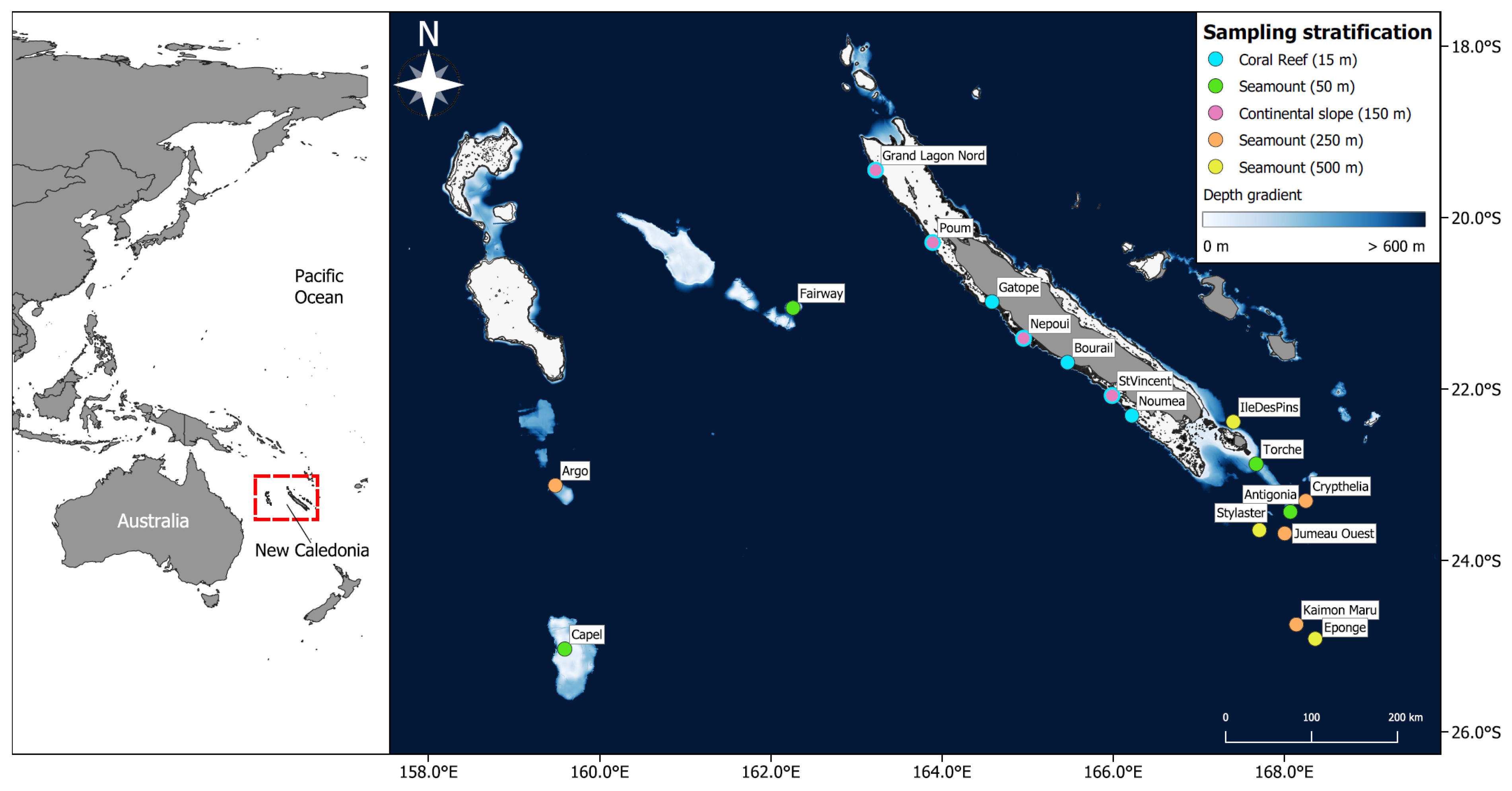
2.1. Data Collection
2.2. Stereo Baited Remote Underwater Video Stations (BRUVS)
2.3. Biomass Estimation
2.4. eDNA Metabarcoding
2.5. eDNA Bioinformatic
2.6. Environmental Variables
2.7. Data Analysis
2.8. Diversity and Biomass Modelling
2.9. Comparisons across Strata
2.10. Assemblages Structure
3. Results
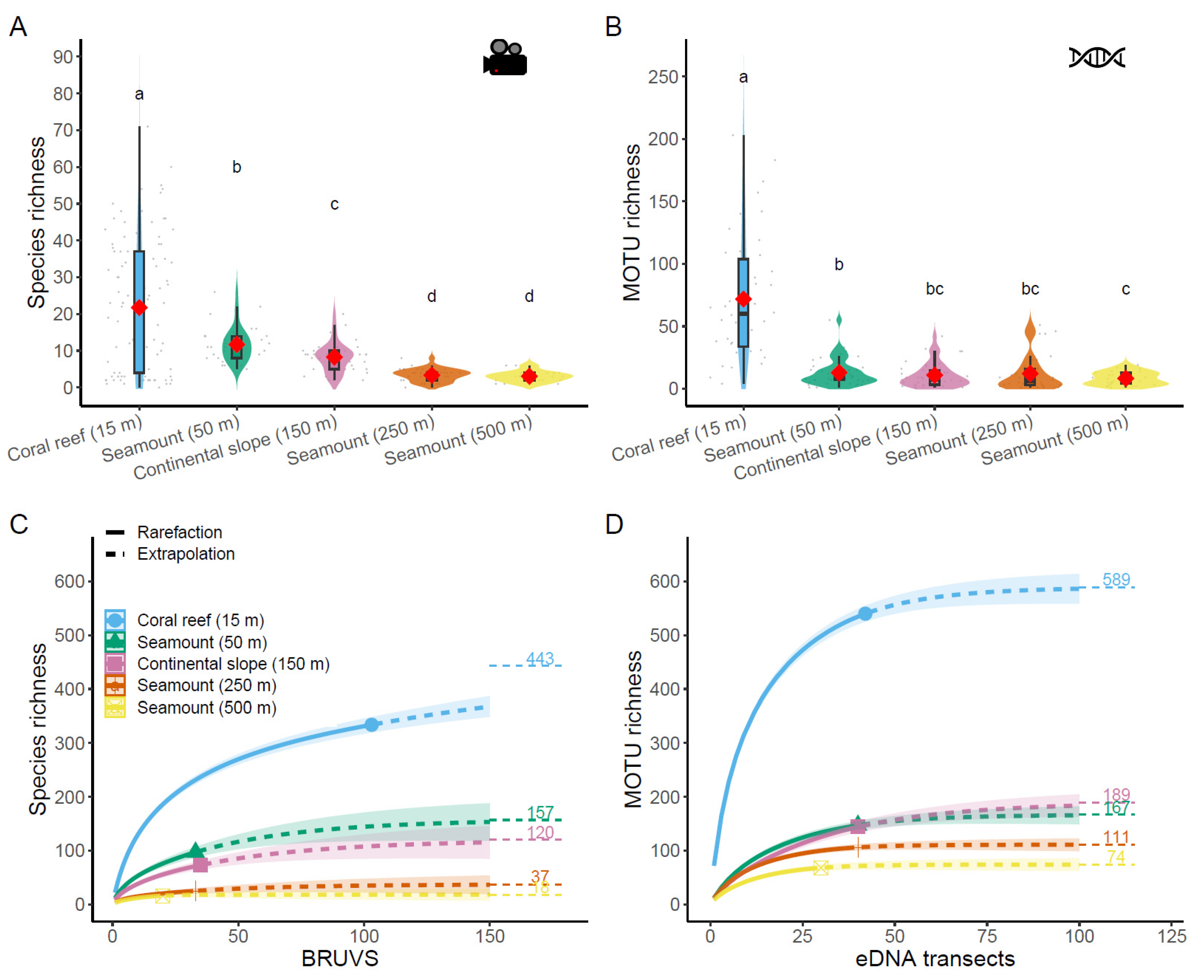
3.1. Biodiversity
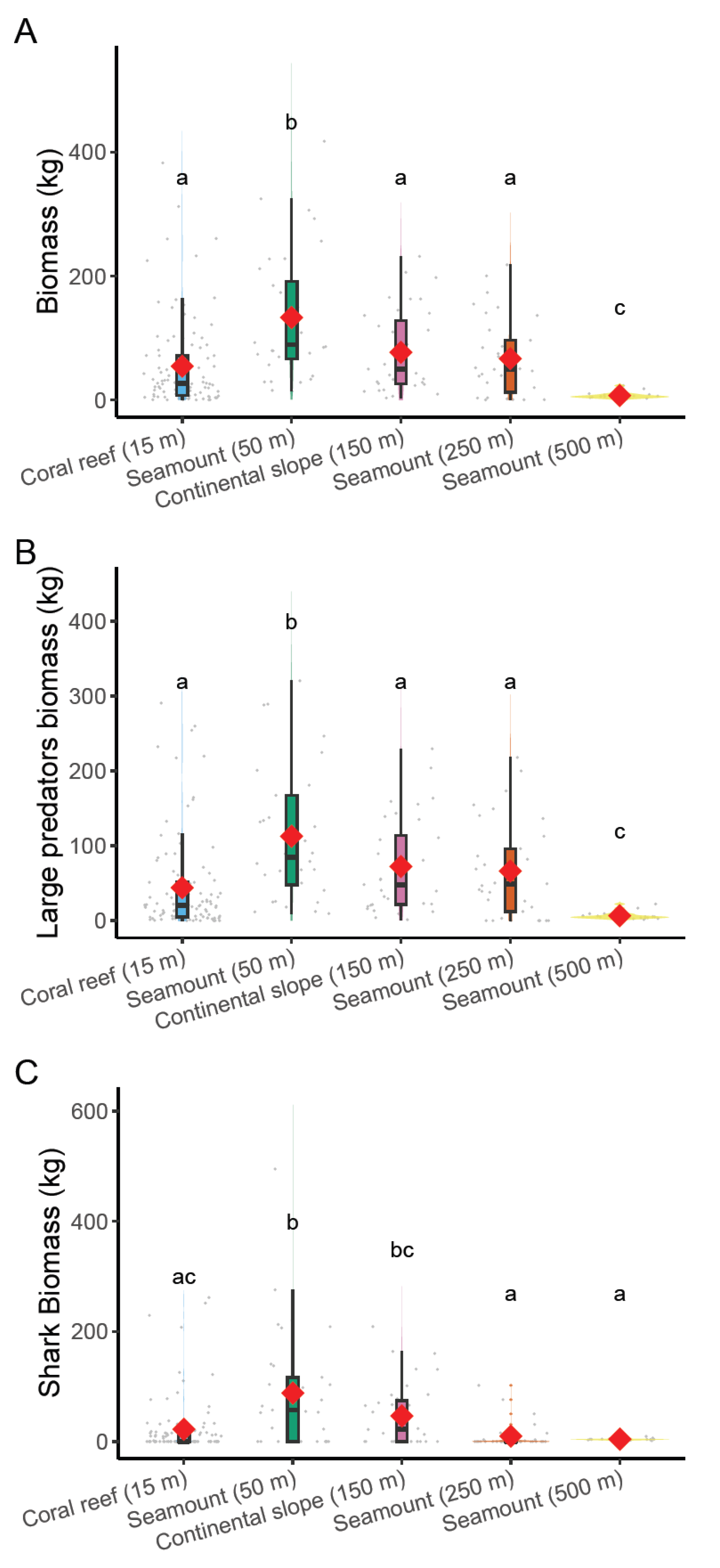
3.2. Biomass
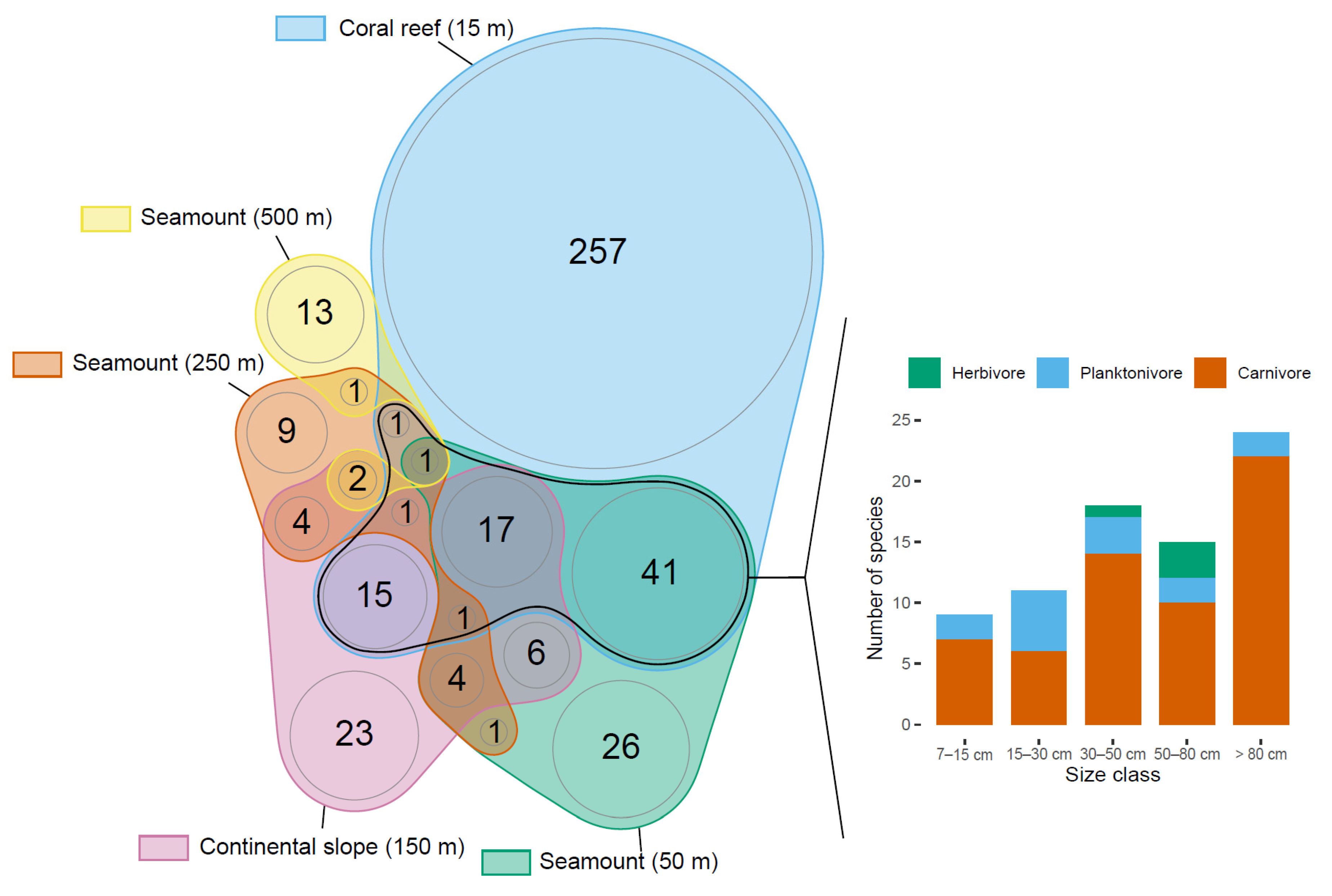
3.3. Assemblage Structure
4. Discussion
5. Conclusions
Supplementary Materials
Author Contributions
Funding
Institutional Review Board Statement
Informed Consent Statement
Data Availability Statement
Acknowledgments
Conflicts of Interest
References
- Kvile, K.Ø.; Taranto, G.H.; Pitcher, T.J.; Morato, T. A Global Assessment of Seamount Ecosystems Knowledge Using an Ecosystem Evaluation Framework. Biol. Conserv. 2014, 173, 108–120. [Google Scholar] [CrossRef]
- Morato, T.; Hoyle, S.D.; Allain, V.; Nicol, S.J. Seamounts Are Hotspots of Pelagic Biodiversity in the Open Ocean. Proc. Natl. Acad. Sci. USA 2010, 107, 9707–9711. [Google Scholar] [CrossRef] [PubMed]
- Samadi, S.; Bottan, L.; Macpherson, E.; de Forges, B.R.; Boisselier, M.C. Seamount Endemism Questioned by the Geographic Distribution and Population Genetic Structure of Marine Invertebrates. Mar. Biol. 2006, 149, 1463–1475. [Google Scholar] [CrossRef]
- Rowden, A.A.; Schlacher, T.A.; Williams, A.; Clark, M.R.; Stewart, R.; Althaus, F.; Bowden, D.A.; Consalvey, M.; Robinson, W.; Dowdney, J. A Test of the Seamount Oasis Hypothesis: Seamounts Support Higher Epibenthic Megafaunal Biomass than Adjacent Slopes. Mar. Ecol. 2010, 31, 95–106. [Google Scholar] [CrossRef]
- Letessier, T.B.; Mouillot, D.; Bouchet, P.J.; Vigliola, L.; Fernandes, M.C.; Thompson, C.; Boussarie, G.; Turner, J.; Juhel, J.-B.; Maire, E.; et al. Remote Reefs and Seamounts Are the Last Refuges for Marine Predators across the Indo-Pacific. PLoS Biol. 2019, 17, e3000366. [Google Scholar] [CrossRef]
- Rogers, A.D. The Biology of Seamounts: 25 Years On. In Advances in Marine Biology; Elsevier: Amsterdam, The Netherlands, 2018; Volume 79, pp. 137–224. ISBN 9780128151013. [Google Scholar]
- Salmerón, F.; Báez, J.; Macías, D.; Fernandez-Peralta, L.; Ramos, A. Rapid Fish Stock Depletion in Previously Unexploited Seamounts: The Case of Beryx Splendens from the Sierra Leone Rise (Gulf of Guinea). Afr. J. Mar. Sci. 2015, 37, 405–409. [Google Scholar] [CrossRef]
- Payne, J.L.; Bush, A.M.; Heim, N.A.; Knope, M.L.; McCauley, D.J. Ecological Selectivity of the Emerging Mass Extinction in the Oceans. Science 2016, 353, 1284–1286. [Google Scholar] [CrossRef]
- Yesson, C.; Clark, M.R.; Taylor, M.L.; Rogers, A.D. The Global Distribution of Seamounts Based on 30 Arc Seconds Bathymetry Data. Deep. Sea Res. Part I Oceanogr. Res. Pap. 2011, 58, 442–453. [Google Scholar] [CrossRef]
- Staudigel, H.; Koppers, A.; Lavelle, J.W.; Pitcher, T.; Shank, T. Defining the Word “Seamount”. Oceanography 2010, 23, 20–21. [Google Scholar] [CrossRef]
- Barnett, A.; AbrantesKá, K.G.; Seymour, J.; Fitzpatrick, R. Residency and Spatial Use by Reef Sharks of an Isolated Seamount and Its Implications for Conservation. PLoS ONE 2012, 7, e0036574. [Google Scholar] [CrossRef]
- Cambra, M.; Lara-Lizardi, F.; Peñaherrera-Palma, C.; Hearn, A.; Ketchum, J.T.; Zarate, P.; Chacón, C.; Suárez-Moncada, J.; Herrera, E.; Espinoza, M. A First Assessment of the Distribution and Abundance of Large Pelagic Species at Cocos Ridge Seamounts (Eastern Tropical Pacific) Using Drifting Pelagic Baited Remote Cameras. PLoS ONE 2021, 16, e0244343. [Google Scholar] [CrossRef]
- Zeppilli, D.; Bongiorni, L.; Santos, R.S.; Vanreusel, A. Changes in Nematode Communities in Different Physiographic Sites of the Condor Seamount (North-East Atlantic Ocean) and Adjacent Sediments. PLoS ONE 2014, 9, e0115601. [Google Scholar] [CrossRef] [PubMed]
- Leitner, A.B.; Neuheimer, A.B.; Drazen, J.C. Evidence for Long-Term Seamount-Induced Chlorophyll Enhancements. Sci. Rep. 2020, 10, 12729. [Google Scholar] [CrossRef] [PubMed]
- Lavelle, J.W.; Mohn, C. Motion, Commotion, and Biophysical Connections at Deep Ocean Seamounts. Oceanography 2010, 23, 90–103. [Google Scholar] [CrossRef]
- Rowden, A.A.; Dower, J.F.; Schlacher, T.A.; Consalvey, M.; Clark, M.R. Paradigms in Seamount Ecology: Fact, Fiction and Future. Mar. Ecol. 2010, 31, 226–241. [Google Scholar] [CrossRef]
- Myers, N.; Mittermeier, R.A.; Mittermeier, C.G.; da Fonseca, G.A.B.; Kent, J. Biodiversity Hotspots for Conservation Priorities. Nature 2000, 403, 853–858. [Google Scholar] [CrossRef] [PubMed]
- Roberts, C.M.; McClean, C.J.; Veron, J.E.N.; Hawkins, J.P.; Allen, G.R.; McAllister, D.E.; Mittermeier, C.G.; Schueler, F.W.; Spalding, M.; Wells, F.; et al. Marine Biodiversity Hotspots and Conservation Priorities for Tropical Reefs. Science 2002, 295, 1280–1284. [Google Scholar] [CrossRef] [PubMed]
- Mittermeier, R.A.; Turner, W.R.; Larsen, F.W.; Brooks, T.M.; Gascon, C. Biodiversity Hotspots; Zachos, F.E., Habel, J.C., Eds.; Springer: Berlin/Heidelberg, Germany, 2011; ISBN 978-3-642-20991-8. [Google Scholar]
- McClanahan, T.R.; Graham, N.A.J.; MacNeil, M.A.; Muthiga, N.A.; Cinner, J.E.; Bruggemann, J.H.; Wilson, S.K. Critical Thresholds and Tangible Targets for Ecosystem-Based Management of Coral Reef Fisheries. Proc. Natl. Acad. Sci. USA 2011, 108, 17230–17233. [Google Scholar] [CrossRef]
- Duffy, J.E.; Lefcheck, J.S.; Stuart-Smith, R.D.; Navarrete, S.A.; Edgar, G.J. Biodiversity Enhances Reef Fish Biomass and Resistance to Climate Change. Proc. Natl. Acad. Sci. USA 2016, 113, 6230–6235. [Google Scholar] [CrossRef]
- Ramdani, M.; Elkhiati, N.; Flower, R.J. Lakes of Africa: North of Sahara. In Encyclopedia of Inland Waters; Elsevier: Amsterdam, The Netherlands, 2009; pp. 544–554. ISBN 9780123706263. [Google Scholar]
- Carney, R.S. Consideration of the Oasis Analogy for Chemosynthetic Communities at Gulf of Mexico Hydrocarbon Vents. Geo-Mar. Lett. 1994, 14, 149–159. [Google Scholar] [CrossRef]
- Nyström, M.; Folke, C.; Moberg, F. Coral Reef Disturbance and Resilence in a Human-Dominated Environment. Trends Ecol. Evol. 2000, 15, 413–417. [Google Scholar] [CrossRef]
- de Leo, F.C.; Smith, C.R.; Rowden, A.A.; Bowden, D.A.; Clark, M.R. Submarine Canyons: Hotspots of Benthic Biomass and Productivity in the Deep Sea. In Proceedings of the Royal Society B: Biological Sciences, London, UK, 22 September 2010; Volume 277, pp. 2783–2792. [Google Scholar]
- Samimi-Namin, K.; Hoeksema, B.W. Hidden Depths: A Unique Biodiversity Oasis in the Persian Gulf in Need of Further Exploration and Conservation. Diversity 2023, 15, 779. [Google Scholar] [CrossRef]
- Sedell, J.R.; Reeves, G.H.; Hauer, F.R.; Stanford, J.A.; Hawkins, C.P. Role of Refugia in Recovery from Disturbances: Modern Fragmented and Disconnected River Systems. Environ. Manag. 1990, 14, 711–724. [Google Scholar] [CrossRef]
- Keppel, G.; van Niel, K.P.; Wardell-Johnson, G.W.; Yates, C.J.; Byrne, M.; Mucina, L.; Schut, A.G.T.; Hopper, S.D.; Franklin, S.E. Refugia: Identifying and Understanding Safe Havens for Biodiversity under Climate Change. Glob. Ecol. Biogeogr. 2012, 21, 393–404. [Google Scholar] [CrossRef]
- Bongaerts, P.; Ridgway, T.; Sampayo, E.M.; Hoegh-Guldberg, O. Assessing the “deep Reef Refugia” Hypothesis: Focus on Caribbean Reefs. Coral Reefs 2010, 29, 309–327. [Google Scholar] [CrossRef]
- Lindfield, S.J.; Harvey, E.S.; Halford, A.R.; McIlwain, J.L. Mesophotic Depths as Refuge Areas for Fishery-Targeted Species on Coral Reefs. Coral Reefs 2016, 35, 125–137. [Google Scholar] [CrossRef]
- Cinner, J.E.; Huchery, C.; MacNeil, M.A.; Graham, N.A.J.; McClanahan, T.R.; Maina, J.; Maire, E.; Kittinger, J.N.; Hicks, C.C.; Mora, C.; et al. Bright Spots among the World’s Coral Reefs. Nature 2016, 535, 416–419. [Google Scholar] [CrossRef]
- Lindfield, S.J.; Mcilwain, J.L.; Harvey, E.S. Depth Refuge and the Impacts of SCUBA Spearfishing on Coral Reef Fishes. PLoS ONE 2014, 9, e92628. [Google Scholar] [CrossRef]
- Bongaerts, P.; Smith, T.B. Beyond the “Deep Reef Refuge” Hypothesis: A Conceptual Framework to Characterize Persistence at Depth. In Mesophotic Coral Ecosystems; Springer: Berlin/Heidelberg, Germany, 2019; pp. 881–895. ISBN 9783319927350. [Google Scholar]
- D’agata, S.; Mouillot, D.; Wantiez, L.; Friedlander, A.M.; Kulbicki, M.; Vigliola, L. Marine Reserves Lag behind Wilderness in the Conservation of Key Functional Roles. Nat. Commun. 2016, 7, 12000. [Google Scholar] [CrossRef]
- Juhel, J.-B.; Vigliola, L.; Mouillot, D.; Kulbicki, M.; Letessier, T.B.; Meeuwig, J.J.; Wantiez, L. Reef Accessibility Impairs the Protection of Sharks. J. Appl. Ecol. 2018, 55, 673–683. [Google Scholar] [CrossRef]
- Januchowski-Hartley, F.A.; Vigliola, L.; Maire, E.; Kulbicki, M.; Mouillot, D. Low Fuel Cost and Rising Fish Price Threaten Coral Reef Wilderness. Conserv. Lett. 2020, 13, 12706. [Google Scholar] [CrossRef]
- Boussarie, G.; Bakker, J.; Wangensteen, O.S.; Mariani, S.; Bonnin, L.; Juhel, J.-B.; Kiszka, J.J.; Kulbicki, M.; Manel, S.; Robbins, W.D.; et al. Environmental DNA Illuminates the Dark Diversity of Sharks. Sci. Adv. 2018, 4, eaap9661. [Google Scholar] [CrossRef]
- Porteiro, F.M.; Gomes-Pereira, J.N.; Pham, C.K.; Tempera, F.; Santos, R.S. Distribution and Habitat Association of Benthic Fish on the Condor Seamount (NE Atlantic, Azores) from in Situ Observations. Deep. Sea Res. Part II Top. Stud. Oceanogr. 2013, 98, 114–128. [Google Scholar] [CrossRef]
- Auzende, J.-M.; Grandperrin, R.; Bouniot, E.; Henin, C.; Lafoy, Y.; Richer de Forges, B.; van de Beuque, S.; Virly, S. Marine Resources of the Economic Zone of New Caledonia. Oceanol. Acta 1999, 22, 557–566. [Google Scholar] [CrossRef]
- Payri, C.E.; Allain, V.; Aucan, J.; David, C.; David, V.; Dutheil, C.; Loubersac, L.; Menkes, C.; Pelletier, B.; Pestana, G. New Caledonia. In World Seas: An Environmental Evaluation; Elsevier: Amsterdam, The Netherlands, 2019; pp. 593–618. [Google Scholar]
- Allain, V.; Kerandel, J.A.; Andréfouët, S.; Magron, F.; Clark, M.; Kirby, D.S.; Muller-Karger, F.E. Enhanced Seamount Location Database for the Western and Central Pacific Ocean: Screening and Cross-Checking of 20 Existing Datasets. Deep Sea Res. Part I Oceanogr. Res. Pap. 2008, 55, 1035–1047. [Google Scholar] [CrossRef]
- Polanco Fernández, A.; Marques, V.; Fopp, F.; Juhel, J.; Borrero-Pérez, G.H.; Cheutin, M.; Dejean, T.; González Corredor, J.D.; Acosta-Chaparro, A.; Hocdé, R.; et al. Comparing Environmental DNA Metabarcoding and Underwater Visual Census to Monitor Tropical Reef Fishes. Environ. DNA 2021, 3, 142–156. [Google Scholar] [CrossRef]
- Deiner, K.; Yamanaka, H.; Bernatchez, L. The Future of Biodiversity Monitoring and Conservation Utilizing Environmental DNA. Environ. DNA 2021, 3, 3–7. [Google Scholar] [CrossRef]
- Valentini, A.; Taberlet, P.; Miaud, C.; Civade, R.; Herder, J.; Thomsen, P.F.; Bellemain, E.; Besnard, A.; Coissac, E.; Boyer, F.; et al. Next-Generation Monitoring of Aquatic Biodiversity Using Environmental DNA Metabarcoding. Mol. Ecol. 2016, 25, 929–942. [Google Scholar] [CrossRef]
- Stat, M.; John, J.; DiBattista, J.D.; Newman, S.J.; Bunce, M.; Harvey, E.S. Combined Use of EDNA Metabarcoding and Video Surveillance for the Assessment of Fish Biodiversity. Conserv. Biol. 2019, 33, 196–205. [Google Scholar] [CrossRef]
- Mathon, L.; Marques, V.; Mouillot, D.; Albouy, C.; Andrello, M.; Baletaud, F.; Borrero-Pérez, G.H.; Dejean, T.; Edgar, G.J.; Grondin, J.; et al. Cross-Ocean Patterns and Processes in Fish Biodiversity on Coral Reefs through the Lens of EDNA Metabarcoding. Proc. R. Soc. B Biol. Sci. 2022, 289, 20220162. [Google Scholar] [CrossRef]
- Whitmarsh, S.K.; Fairweather, P.G.; Huveneers, C. What Is Big BRUVver up to? Methods and Uses of Baited Underwater Video. Rev. Fish Biol. Fish 2017, 27, 53–73. [Google Scholar] [CrossRef]
- Langlois, T.; Goetze, J.; Bond, T.; Monk, J.; Abesamis, R.A.; Asher, J.; Barrett, N.; Bernard, A.T.F.; Bouchet, P.J.; Birt, M.J.; et al. A Field and Video Annotation Guide for Baited Remote Underwater Stereo-Video Surveys of Demersal Fish Assemblages. Methods Ecol. Evol. 2020, 11, 1401–1409. [Google Scholar] [CrossRef]
- Elith, J.; Leathwick, J.R.; Hastie, T. A Working Guide to Boosted Regression Trees. J. Anim. Ecol. 2008, 77, 802–813. [Google Scholar] [CrossRef] [PubMed]
- Shom-IRD MNT Bathymétrique de Façade de La Nouvelle-Calédonie (Projet TSUCAL). 2021. Available online: http://dx.doi.org/10.17183/MNT_NC100m_TSUCAL_WGS84 (accessed on 1 November 2020).
- Letessier, T.B.; Juhel, J.B.; Vigliola, L.; Meeuwig, J.J. Low-Cost Small Action Cameras in Stereo Generates Accurate Underwater Measurements of Fish. J. Exp. Mar. Biol. Ecol. 2015, 466, 120–126. [Google Scholar] [CrossRef]
- Cappo, M.; Harvey, E.; Malcolm, H.; Speare, P. Potential of Video Techniques to Monitor Diversity, Abundance and Size of Fish in Studies of Marine Protected Areas. In Aquatic Protected Areas-What Works Best and How Do We Know? University of Queensland: Brisbane, Australia, 2003; pp. 455–464. [Google Scholar]
- Taylor, R.B.; Willis, T.J. Relationships amongst Length, Weight and Growth of North-Eastern New Zealand Reef Fishes. Mar. Freshw. Res. 1998, 49, 255–260. [Google Scholar] [CrossRef]
- Stekhoven, D.J.; Buhlmann, P. MissForest: Non-Parametric Missing Value Imputation for Mixed-Type Data. Bioinformatics 2012, 28, 112–118. [Google Scholar] [CrossRef]
- Goldberg, C.S.; Turner, C.R.; Deiner, K.; Klymus, K.E.; Thomsen, P.F.; Murphy, M.A.; Spear, S.F.; McKee, A.; Oyler-McCance, S.J.; Cornman, R.S.; et al. Critical Considerations for the Application of Environmental DNA Methods to Detect Aquatic Species. Methods Ecol. Evol. 2016, 7, 1299–1307. [Google Scholar] [CrossRef]
- Mathon, L.; Marques, V.; Manel, S.; Albouy, C.; Andrello, M.; Boulanger, E.; Deter, J.; Hocdé, R.; Leprieur, F.; Letessier, T.B.; et al. The Distribution of Coastal Fish eDNA Sequences in the Anthropocene. Glob. Ecol. Biogeogr. 2023, 32, 1336–1352. [Google Scholar] [CrossRef]
- Marques, V.; Guérin, P.É.; Rocle, M.; Valentini, A.; Manel, S.; Mouillot, D.; Dejean, T. Blind Assessment of Vertebrate Taxonomic Diversity across Spatial Scales by Clustering Environmental DNA Metabarcoding Sequences. Ecography 2020, 43, 1779–1790. [Google Scholar] [CrossRef]
- Rognes, T.; Flouri, T.; Nichols, B.; Quince, C.; Mahé, F. VSEARCH: A Versatile Open Source Tool for Metagenomics. PeerJ 2016, 4, e2584. [Google Scholar] [CrossRef]
- Martin, M. Cutadapt Removes Adapter Sequences from High-Throughput Sequencing Reads. EMBnet. J. 2011, 17, 10. [Google Scholar] [CrossRef]
- Mahé, F.; Rognes, T.; Quince, C.; de Vargas, C.; Dunthorn, M. Swarm v2: Highly-Scalable and High-Resolution Amplicon Clustering. PeerJ 2015, 3, e1420. [Google Scholar] [CrossRef]
- Boyer, F.; Mercier, C.; Bonin, A.; le Bras, Y.; Taberlet, P.; Coissac, E. Obitools: A Unix-Inspired Software Package for DNA Metabarcoding. Mol. Ecol. Resour. 2016, 16, 176–182. [Google Scholar] [CrossRef] [PubMed]
- Leinonen, R.; Akhtar, R.; Birney, E.; Bower, L.; Cerdeno-Tarraga, A.; Cheng, Y.; Cleland, I.; Faruque, N.; Goodgame, N.; Gibson, R.; et al. The European Nucleotide Archive. Nucleic. Acids Res. 2011, 39, D28–D31. [Google Scholar] [CrossRef]
- Schnell, I.B.; Bohmann, K.; Gilbert, M.T.P. Tag Jumps Illuminated-Reducing Sequence-to-Sample Misidentifications in Metabarcoding Studies. Mol. Ecol. Resour. 2015, 15, 1289–1303. [Google Scholar] [CrossRef] [PubMed]
- MacConaill, L.E.; Burns, R.T.; Nag, A.; Coleman, H.A.; Slevin, M.K.; Giorda, K.; Light, M.; Lai, K.; Jarosz, M.; McNeill, M.S.; et al. Unique, Dual-Indexed Sequencing Adapters with UMIs Effectively Eliminate Index Cross-Talk and Significantly Improve Sensitivity of Massively Parallel Sequencing. BMC Genom. 2018, 19. [Google Scholar] [CrossRef]
- Tittensor, D.P.; Mora, C.; Jetz, W.; Lotze, H.K.; Ricard, D.; vanden Berghe, E.; Worm, B. Global Patterns and Predictors of Marine Biodiversity across Taxa. Nature 2010, 466, 1098–1101. [Google Scholar] [CrossRef]
- Currie, D.J.; Mittelbach, G.G.; Cornell, H.v.; Field, R.; Guegan, J.-F.; Hawkins, B.A.; Kaufman, D.M.; Kerr, J.T.; Oberdorff, T.; O’Brien, E.; et al. Predictions and Tests of Climate-Based Hypotheses of Broad-Scale Variation in Taxonomic Richness. Ecol. Lett. 2004, 7, 1121–1134. [Google Scholar] [CrossRef]
- Capblancq, J. Nutrient Dynamics and Pelagic Food Web Interactions in Oligotrophic and Eutrophic Environments: An Overview. Hydrobiologia 1990, 207, 1–14. [Google Scholar] [CrossRef]
- Barletta, M.; Barletta-Bergan, A.; Saint-Paul, U.; Hubold, G. The Role of Salinity in Structuring the Fish Assemblages in a Tropical Estuary. J. Fish Biol. 2005, 66, 45–72. [Google Scholar] [CrossRef]
- Priede, I.G.; Bergstad, O.A.; Miller, P.I.; Vecchione, M.; Gebruk, A.; Falkenhaug, T.; Billett, D.S.M.; Craig, J.; Dale, A.C.; Shields, M.A.; et al. Does Presence of a Mid-Ocean Ridge Enhance Biomass and Biodiversity? PLoS ONE 2013, 8, e0061550. [Google Scholar] [CrossRef]
- Maire, E.; Cinner, J.; Velez, L.; Huchery, C.; Mora, C.; Dagata, S.; Vigliola, L.; Wantiez, L.; Kulbicki, M.; Mouillot, D. How Accessible Are Coral Reefs to People? A Global Assessment Based on Travel Time. Ecol. Lett. 2016, 19, 351–360. [Google Scholar] [CrossRef] [PubMed]
- Clua, E.; Legendre, P.; Vigliola, L.; Magron, F.; Kulbicki, M.; Sarramegna, S.; Labrosse, P.; Galzin, R. Medium Scale Approach (MSA) for Improved Assessment of Coral Reef Fish Habitat. J. Exp. Mar. Biol. Ecol. 2006, 333, 219–230. [Google Scholar] [CrossRef]
- Baletaud, F.; Gilbert, A.; Mouillot, D.; Come, J.-M.; Vigliola, L. Baited Video Reveal Fish Diversity in the Vast Inter-Reef Habitats of a Marine Tropical Lagoon. Mar. Biodivers. 2022, 52, 16. [Google Scholar] [CrossRef]
- Eduardo, L.N.; Frédou, T.; Lira, A.S.; Ferreira, B.P.; Bertrand, A.; Ménard, F.; Frédou, F.L. Identifying Key Habitat and Spatial Patterns of Fish Biodiversity in the Tropical Brazilian Continental Shelf. Cont. Shelf. Res. 2018, 166, 108–118. [Google Scholar] [CrossRef]
- Sih, T.; Daniell, J.; Bridge, T.; Beaman, R.; Cappo, M.; Kingsford, M. Deep-Reef Fish Communities of the Great Barrier Reef Shelf-Break: Trophic Structure and Habitat Associations. Diversity 2019, 11, 26. [Google Scholar] [CrossRef]
- Mouillot, D.; Villeger, S.; Parravicini, V.; Kulbicki, M.; Arias-Gonzalez, J.E.; Bender, M.; Chabanet, P.; Floeter, S.R.; Friedlander, A.; Vigliola, L.; et al. Functional Over-Redundancy and High Functional Vulnerability in Global Fish Faunas on Tropical Reefs. Proc. Natl. Acad. Sci. USA 2014, 111, 13757–13762. [Google Scholar] [CrossRef]
- R Core Team. R: A Language and Environment for Statistical Computing; R Foundation for Statistical Computing: Vienna, Austria, 2021. [Google Scholar]
- Anderson, M.J. A New Method for Non-Parametric Multivariate Analysis of Variance. Austral. Ecol. 2001, 26, 32–46. [Google Scholar] [CrossRef]
- Chao, A.; Gotelli, N.J.; Hsieh, T.C.; Sander, E.L.; Ma, K.H.; Colwell, R.K.; Ellison, A.M. Rarefaction and Extrapolation with Hill Numbers: A Framework for Sampling and Estimation in Species Diversity Studies. Ecol. Monogr. 2014, 84, 45–67. [Google Scholar] [CrossRef]
- Hsieh, T.C.; Ma, K.H.; Chao, A. INEXT: An R Package for Rarefaction and Extrapolation of Species Diversity (Hill Numbers). Methods Ecol. Evol. 2016, 7, 1451–1456. [Google Scholar] [CrossRef]
- Legendre, P.; Legendre, L. Numerical Ecology: Second English Edition; Elsevier Science: Amsterdam, The Netherlands, 1998; Volume 20. [Google Scholar]
- Dorman, S.R.; Harvey, E.S.; Newman, S.J. Bait Effects in Sampling Coral Reef Fish Assemblages with Stereo-BRUVs. PLoS ONE 2012, 7, e0041538. [Google Scholar] [CrossRef] [PubMed]
- Cheal, A.J.; Emslie, M.J.; Currey-Randall, L.M.; Heupel, M.R. Comparability and Complementarity of Reef Fish Measures from Underwater Visual Census (UVC) and Baited Remote Underwater Video Stations (BRUVS). J. Environ. Manag. 2021, 289, 112375. [Google Scholar] [CrossRef] [PubMed]
- Abesamis, R.A.; Utzurrum, J.A.T.; Raterta, L.J.J.; Russ, G.R. Shore-Fish Assemblage Structure in the Central Philippines from Shallow Coral Reefs to the Mesophotic Zone. Mar Biol 2020, 167, 185. [Google Scholar] [CrossRef]
- Andradi-Brown, D.A.; Macaya-Solis, C.; Exton, D.A.; Gress, E.; Wright, G.; Rogers, A.D. Assessing Caribbean Shallow and Mesophotic Reef Fish Communities Using Baited-Remote Underwater Video (BRUV) and Diver-Operated Video (DOV) Survey Techniques. PLoS ONE 2016, 11, e0168235. [Google Scholar] [CrossRef] [PubMed]
- Barley, S.; Meekan, M.; Meeuwig, J. Species Diversity, Abundance, Biomass, Size and Trophic Structure of Fish on Coral Reefs in Relation to Shark Abundance. Mar. Ecol. Prog. Ser. 2017, 565, 163–179. [Google Scholar] [CrossRef]
- Leitner, A.B.; Durden, J.M.; Smith, C.R.; Klingberg, E.D.; Drazen, J.C. Synaphobranchid Eel Swarms on Abyssal Seamounts: Largest Aggregation of Fishes Ever Observed at Abyssal Depths. Deep Sea Res. Part I Oceanogr. Res. Pap. 2021, 167, 103423. [Google Scholar] [CrossRef]
- Fitzpatrick, B.M.; Harvey, E.S.; Heyward, A.J.; Twiggs, E.J.; Colquhoun, J. Habitat Specialization in Tropical Continental Shelf Demersal Fish Assemblages. PLoS ONE 2012, 7, e39634. [Google Scholar] [CrossRef]
- Pearson, R.; Stevens, T. Distinct Cross-Shelf Gradient in Mesophotic Reef Fish Assemblages in Subtropical Eastern Australia. Mar. Ecol. Prog. Ser. 2015, 532, 185–196. [Google Scholar] [CrossRef]
- Abesamis, R.A.; Langlois, T.; Birt, M.; Thillainath, E.; Bucol, A.A.; Arceo, H.O.; Russ, G.R. Benthic Habitat and Fish Assemblage Structure from Shallow to Mesophotic Depths in a Storm-Impacted Marine Protected Area. Coral Reefs 2018, 37, 81–97. [Google Scholar] [CrossRef]
- Wang, S.; Yan, Z.; Hänfling, B.; Zheng, X.; Wang, P.; Fan, J.; Li, J. Methodology of Fish EDNA and Its Applications in Ecology and Environment. Sci. Total Environ. 2021, 755, 142622. [Google Scholar] [CrossRef]
- Evans, N.T.; Li, Y.; Renshaw, M.A.; Olds, B.P.; Deiner, K.; Turner, C.R.; Jerde, C.L.; Lodge, D.M.; Lamberti, G.A.; Pfrender, M.E. Fish Community Assessment with EDNA Metabarcoding: Effects of Sampling Design and Bioinformatic Filtering. Can. J. Fish. Aquat. Sci. 2017, 74, 1362–1374. [Google Scholar] [CrossRef]
- Marques, V.; Castagné, P.; Polanco, A.; Borrero-Pérez, G.H.; Hocdé, R.; Guérin, P.É.; Juhel, J.B.; Velez, L.; Loiseau, N.; Letessier, T.B.; et al. Use of Environmental DNA in Assessment of Fish Functional and Phylogenetic Diversity. Conserv. Biol. 2021, 35, 1944–1956. [Google Scholar] [CrossRef]
- McClenaghan, B.; Fahner, N.; Cote, D.; Chawarski, J.; McCarthy, A.; Rajabi, H.; Singer, G.; Hajibabaei, M. Harnessing the Power of EDNA Metabarcoding for the Detection of Deep-Sea Fishes. PLoS ONE 2020, 15, e0236540. [Google Scholar] [CrossRef] [PubMed]
- Goatley, C.H.R.; Brandl, S.J. Cryptobenthic Reef Fishes. Curr. Biol. 2017, 27, R452–R454. [Google Scholar] [CrossRef]
- Stat, M.; Huggett, M.J.; Bernasconi, R.; DiBattista, J.D.; Berry, T.E.; Newman, S.J.; Harvey, E.S.; Bunce, M. Ecosystem Biomonitoring with EDNA: Metabarcoding across the Tree of Life in a Tropical Marine Environment. Sci. Rep. 2017, 7, 12240. [Google Scholar] [CrossRef]
- Cappo, M.; Speare, P.; De’ath, G. Comparison of Baited Remote Underwater Video Stations (BRUVS) and Prawn (Shrimp) Trawls for Assessments of Fish Biodiversity in Inter-Reefal Areas of the Great Barrier Reef Marine Park. J. Exp. Mar. Biol. Ecol. 2004, 302, 123–152. [Google Scholar] [CrossRef]
- Marchese, C. Biodiversity Hotspots: A Shortcut for a More Complicated Concept. Glob. Ecol. Conserv. 2015, 3, 297–309. [Google Scholar] [CrossRef]
- Hughes, T.P.; Barnes, M.L.; Bellwood, D.R.; Cinner, J.E.; Cumming, G.S.; Jackson, J.B.C.; Kleypas, J.; van de Leemput, I.A.; Lough, J.M.; Morrison, T.H.; et al. Coral Reefs in the Anthropocene. Nature 2017, 546, 82–90. [Google Scholar] [CrossRef]
- Halpern, B.S.; Frazier, M.; Afflerbach, J.; Lowndes, J.S.; Micheli, F.; O’Hara, C.; Scarborough, C.; Selkoe, K.A. Recent Pace of Change in Human Impact on the World’s Ocean. Sci. Rep. 2019, 9, 11609. [Google Scholar] [CrossRef]
- Morato, T.; Watson, R.; Pitcher, T.J.; Pauly, D. Fishing down the Deep. Fish Fish. 2006, 7, 24–34. [Google Scholar] [CrossRef]
- Tillin, H.; Hiddink, J.; Jennings, S.; Kaiser, M. Chronic Bottom Trawling Alters the Functional Composition of Benthic Invertebrate Communities on a Sea-Basin Scale. Mar. Ecol. Prog. Ser. 2006, 318, 31–45. [Google Scholar] [CrossRef]
- Thrush, S.F.; Dayton, P.K. Disturbance to Marine Benthic Habitats by Trawling and Dredging: Implications for Marine Biodiversity. Annu. Rev. Ecol. Syst. 2002, 33, 449–473. [Google Scholar] [CrossRef]
- Williams, A.; Schlacher, T.A.; Rowden, A.A.; Althaus, F.; Clark, M.R.; Bowden, D.A.; Stewart, R.; Bax, N.J.; Consalvey, M.; Kloser, R.J. Seamount Megabenthic Assemblages Fail to Recover from Trawling Impacts. Mar. Ecol. 2010, 31, 183–199. [Google Scholar] [CrossRef]
- Althaus, F.; Williams, A.; Schlacher, T.A.; Kloser, R.J.; Green, M.A.; Barker, B.A.; Bax, N.J.; Brodie, P.; Schlacher-Hoenlinger, M.A. Impacts of Bottom Trawling on Deep-Coral Ecosystems of Seamounts Are Long-Lasting. Mar. Ecol. Prog. Ser. 2009, 397, 279–294. [Google Scholar] [CrossRef]
- West, K.M.; Stat, M.; Harvey, E.S.; Skepper, C.L.; DiBattista, J.D.; Richards, Z.T.; Travers, M.J.; Newman, S.J.; Bunce, M. EDNA Metabarcoding Survey Reveals Fine-Scale Coral Reef Community Variation across a Remote, Tropical Island Ecosystem. Mol. Ecol. 2020, 29, 1069–1086. [Google Scholar] [CrossRef]
- Danovaro, R.; Snelgrove, P.V.R.; Tyler, P. Challenging the Paradigms of Deep-Sea Ecology. Trends Ecol. Evol. 2014, 29, 465–475. [Google Scholar] [CrossRef]
- Wellington, C.M.; Harvey, E.S.; Wakefield, C.B.; Langlois, T.J.; Williams, A.; White, W.T.; Newman, S.J. Peak in Biomass Driven by Larger-Bodied Meso-Predators in Demersal Fish Communities between Shelf and Slope Habitats at the Head of a Submarine Canyon in the South-Eastern Indian Ocean. Cont. Shelf. Res. 2018, 167, 55–64. [Google Scholar] [CrossRef]
- Rogers, A.; Blanchard, J.L.; Mumby, P.J. Vulnerability of Coral Reef Fisheries to a Loss of Structural Complexity. Curr. Biol. 2014, 24, 1000–1005. [Google Scholar] [CrossRef]
- Moura, R.L.; Abieri, M.L.; Castro, G.M.; Carlos-Júnior, L.A.; Chiroque-Solano, P.M.; Fernandes, N.C.; Teixeira, C.D.; Ribeiro, F.V.; Salomon, P.S.; Freitas, M.O.; et al. Tropical Rhodolith Beds Are a Major and Belittled Reef Fish Habitat. Sci. Rep. 2021, 11, 794. [Google Scholar] [CrossRef]
- Pauly, D.; Christensen, V.; Dalsgaard, J.; Froese, R.; Torres, F., Jr. Fishing down the Food Webs. Science 1998, 279, 860–863. [Google Scholar] [CrossRef]
- Pauly, D.; Zeller, D. Catch Reconstructions Reveal That Global Marine Fisheries Catches Are Higher than Reported and Declining. Nat. Commun. 2016, 7, 10244. [Google Scholar] [CrossRef] [PubMed]
- Ripple, W.J.; Wolf, C.; Newsome, T.M.; Betts, M.G.; Ceballos, G.; Courchamp, F.; Hayward, M.W.; van Valkenburgh, B.; Wallach, A.D.; Worm, B. Are We Eating the World’s Megafauna to Extinction? Conserv. Lett. 2019, 12, 1–10. [Google Scholar] [CrossRef]
- Drazen, J.C.; Sutton, T.T. Dining in the Deep: The Feeding Ecology of Deep-Sea Fishes. Ann. Rev. Mar. Sci. 2017, 9, 337–366. [Google Scholar] [CrossRef] [PubMed]
- Bakker, J.; Wangensteen, O.S.; Chapman, D.D.; Boussarie, G.; Buddo, D.; Guttridge, T.L.; Hertler, H.; Mouillot, D.; Vigliola, L.; Mariani, S. Environmental DNA Reveals Tropical Shark Diversity in Contrasting Levels of Anthropogenic Impact. Sci. Rep. 2017, 7, 16886. [Google Scholar] [CrossRef]
- Hemingson, C.R.; Bellwood, D.R. Biogeographic Patterns in Major Marine Realms: Function Not Taxonomy Unites Fish Assemblages in Reef, Seagrass and Mangrove Systems. Ecography 2018, 41, 174–182. [Google Scholar] [CrossRef]
- Collins, R.A.; Wangensteen, O.S.; O’Gorman, E.J.; Mariani, S.; Sims, D.W.; Genner, M.J. Persistence of Environmental DNA in Marine Systems. Commun. Biol. 2018, 1, 185. [Google Scholar] [CrossRef]
- Hansen, B.K.; Bekkevold, D.; Clausen, L.W.; Nielsen, E.E. The Sceptical Optimist: Challenges and Perspectives for the Application of Environmental DNA in Marine Fisheries. Fish Fish. 2018, 19, 751–768. [Google Scholar] [CrossRef]
- Jeunen, G.J.; Knapp, M.; Spencer, H.G.; Lamare, M.D.; Taylor, H.R.; Stat, M.; Bunce, M.; Gemmell, N.J. Environmental DNA (EDNA) Metabarcoding Reveals Strong Discrimination among Diverse Marine Habitats Connected by Water Movement. Mol. Ecol. Resour. 2019, 19, 426–438. [Google Scholar] [CrossRef]
- Nguyen, B.N.; Shen, E.W.; Seemann, J.; Correa, A.M.S.; O’Donnell, J.L.; Altieri, A.H.; Knowlton, N.; Crandall, K.A.; Egan, S.P.; McMillan, W.O.; et al. Environmental DNA Survey Captures Patterns of Fish and Invertebrate Diversity across a Tropical Seascape. Sci. Rep. 2020, 10, 185. [Google Scholar] [CrossRef]
- Tribot, A.-S.; Carabeux, Q.; Deter, J.; Claverie, T.; Villéger, S.; Mouquet, N. Confronting Species Aesthetics with Ecological Functions in Coral Reef Fish. Sci. Rep. 2018, 8, 11733. [Google Scholar] [CrossRef]
- Tribot, A.-S.; Deter, J.; Claverie, T.; Guillhaumon, F.; Villéger, S.; Mouquet, N. Species Diversity and Composition Drive the Aesthetic Value of Coral Reef Fish Assemblages. Biol. Lett. 2019, 15, 20190703. [Google Scholar] [CrossRef] [PubMed]
- Holmlund, C.M.; Hammer, M. Ecosystem Services Generated by Fish Populations. Ecol. Econ. 1999, 29, 253–268. [Google Scholar] [CrossRef]
- Worm, B.; Barbier, E.B.; Beaumont, N.; Duffy, J.E.; Folke, C.; Halpern, B.S.; Jackson, J.B.C.; Lotze, H.K.; Micheli, F.; Palumbi, S.R.; et al. Impacts of Biodiversity Loss on Ocean Ecosystem Services. Science 2006, 314, 787–790. [Google Scholar] [CrossRef] [PubMed]
- Brandl, S.J.; Rasher, D.B.; Côté, I.M.; Casey, J.M.; Darling, E.S.; Lefcheck, J.S.; Duffy, J.E. Coral Reef Ecosystem Functioning: Eight Core Processes and the Role of Biodiversity. Front. Ecol. Environ. 2019, 17, 445–454. [Google Scholar] [CrossRef]
- Pecl, G.T.; Araújo, M.B.; Bell, J.D.; Blanchard, J.; Bonebrake, T.C.; Chen, I.C.; Clark, T.D.; Colwell, R.K.; Danielsen, F.; Evengård, B.; et al. Biodiversity Redistribution under Climate Change: Impacts on Ecosystems and Human Well-Being. Science 2017, 355, 6332. [Google Scholar] [CrossRef]
- Ceballos, G.; Ehrlich, P.R.; Dirzo, R. Biological Annihilation via the Ongoing Sixth Mass Extinction Signaled by Vertebrate Population Losses and Declines. Proc. Natl. Acad. Sci. USA 2017, 114, E6089–E6096. [Google Scholar] [CrossRef] [PubMed]
- Soulé, M.E. What Is Conservation Biology? Bioscience 1985, 35, 727–734. [Google Scholar]
- Boettiger, C.; Lang, D.T.; Wainwright, P.C. rfishbase: Exploring, manipulating and visualizing FishBase data from R. J. Fish Biol. 2012, 81, 2030–2039. [Google Scholar] [CrossRef]
- Woolley, S.N.C.; Tittensor, D.P.; Dunstan, P.K.; Guillera-Arroita, G.; Lahoz-Monfort, J.J.; Wintle, B.A.; Worm, B.; O’Hara, T.D. Deep-sea diversity patterns are shaped by energy availability. Nature 2016, 533, 393–396. [Google Scholar] [CrossRef]


| BRT Model | NT | TC | LR | BF | CV (SD) | Variables | Variable Importance |
|---|---|---|---|---|---|---|---|
| Species richness | 1050 | 4 | 0.005 | 0.5 | 0.89 | Depth | 76.5% |
| (BRUVS) | (0.01) | Habitat diversity | 15.7% | ||||
| Mean SST | 7.8% | ||||||
| MOTU richness | 700 | 4 | 0.01 | 0.75 | 0.86 | Depth | 74.8% |
| (eDNA) | (0.05) | Chla | 11.9% | ||||
| Travel time | 6.7% | ||||||
| Northward velocity | 6.6% | ||||||
| Total biomass | 2875 | 5 | 0.001 | 0.75 | 0.73 | Depth | 36.7% |
| (BRUVS) | (0.03) | Habitat diversity | 23.6% | ||||
| Travel time | 11.7% | ||||||
| Eastward velocity | 8.5% | ||||||
| Chla | 8.1% | ||||||
| Northward velocity | 5.9% | ||||||
| Mean SST | 5.5% | ||||||
| Large predators’ biomass | 2825 | 5 | 0.001 | 0.75 | 0.71 | Depth | 26.1% |
| (BRT) | (0.03) | Habitat diversity | 19.6% | ||||
| Travel time | 15.0% | ||||||
| Eastward velocity | 8.7% | ||||||
| Chla | 8.6% | ||||||
| Mean SST | 8.4% | ||||||
| Environmental stratum | 6.9% | ||||||
| Northward velocity | 6.8% |
Disclaimer/Publisher’s Note: The statements, opinions and data contained in all publications are solely those of the individual author(s) and contributor(s) and not of MDPI and/or the editor(s). MDPI and/or the editor(s) disclaim responsibility for any injury to people or property resulting from any ideas, methods, instructions or products referred to in the content. |
© 2023 by the authors. Licensee MDPI, Basel, Switzerland. This article is an open access article distributed under the terms and conditions of the Creative Commons Attribution (CC BY) license (https://creativecommons.org/licenses/by/4.0/).
Share and Cite
Baletaud, F.; Lecellier, G.; Gilbert, A.; Mathon, L.; Côme, J.-M.; Dejean, T.; Dumas, M.; Fiat, S.; Vigliola, L. Comparing Seamounts and Coral Reefs with eDNA and BRUVS Reveals Oases and Refuges on Shallow Seamounts. Biology 2023, 12, 1446. https://doi.org/10.3390/biology12111446
Baletaud F, Lecellier G, Gilbert A, Mathon L, Côme J-M, Dejean T, Dumas M, Fiat S, Vigliola L. Comparing Seamounts and Coral Reefs with eDNA and BRUVS Reveals Oases and Refuges on Shallow Seamounts. Biology. 2023; 12(11):1446. https://doi.org/10.3390/biology12111446
Chicago/Turabian StyleBaletaud, Florian, Gaël Lecellier, Antoine Gilbert, Laëtitia Mathon, Jean-Marie Côme, Tony Dejean, Mahé Dumas, Sylvie Fiat, and Laurent Vigliola. 2023. "Comparing Seamounts and Coral Reefs with eDNA and BRUVS Reveals Oases and Refuges on Shallow Seamounts" Biology 12, no. 11: 1446. https://doi.org/10.3390/biology12111446