
A Boundary-Enhanced Liver Segmentation Network for Multi-Phase CT Images with Unsupervised Domain Adaptation
 , , ,
, , ,
Abstract
:1. Introduction
- We propose a novel domain adaptation framework [18] with dual discriminators operating at two levels, incorporating adaptation both at the feature level and at the output level.
- We introduce an additional boundary-enhanced decoder to determine the boundary loss along with the segmentation loss. The advantage of this approach is that during inference this additional decoder can be dropped, and use the encoder and decoder-1 network to perform liver segmentation. This approach is cost-effective and can be combined with any network.
- We propose using a boundary-enhanced segmentation network as the generator of our proposed DD-UDA framework to perform liver segmentation on a well-annotated source domain (public dataset) and an unannotated target domain (private dataset). We performed several experiments, and our experimental results show that our proposed framework can achieve significantly improved results compared to other state-of-the-art methods.
2. Related Works
2.1. Deep Learning-Based Segmentation Method
2.2. Unsupervised Domain Adaptation
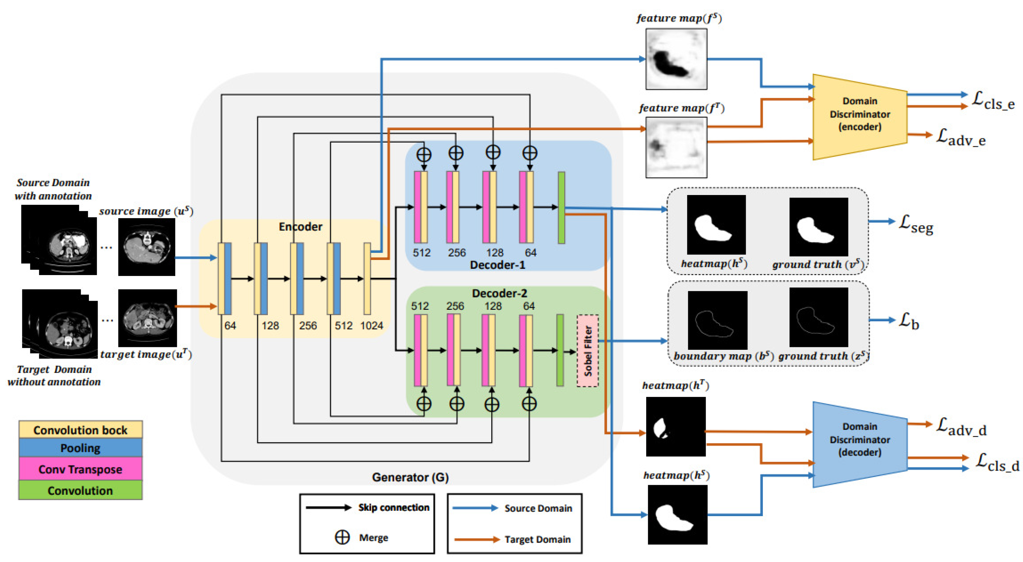
3. Method

3.1. Formal Description
3.2. Boundary-Enhanced Segmentation Network (Generator)
3.2.1. Segmentation Loss
3.2.2. Boundary Loss
3.3. Dual Discriminator-Based Unsupervised Domain Adaptation Using Adversarial Learning
3.3.1. Adversarial Loss
3.3.2. Classification Loss
3.4. Objective Function
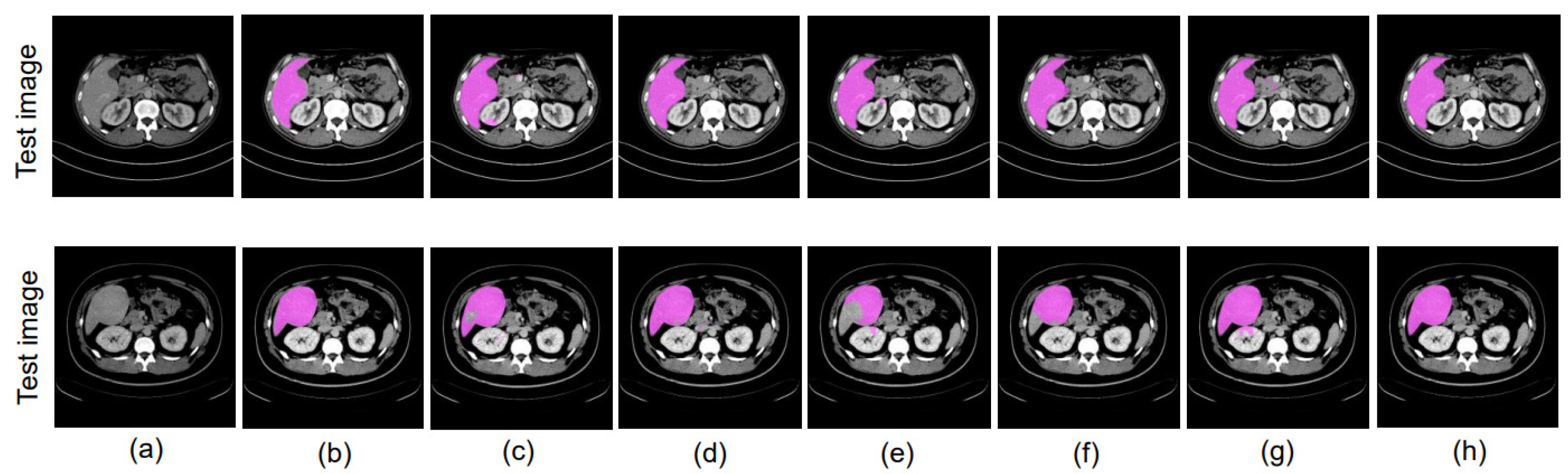
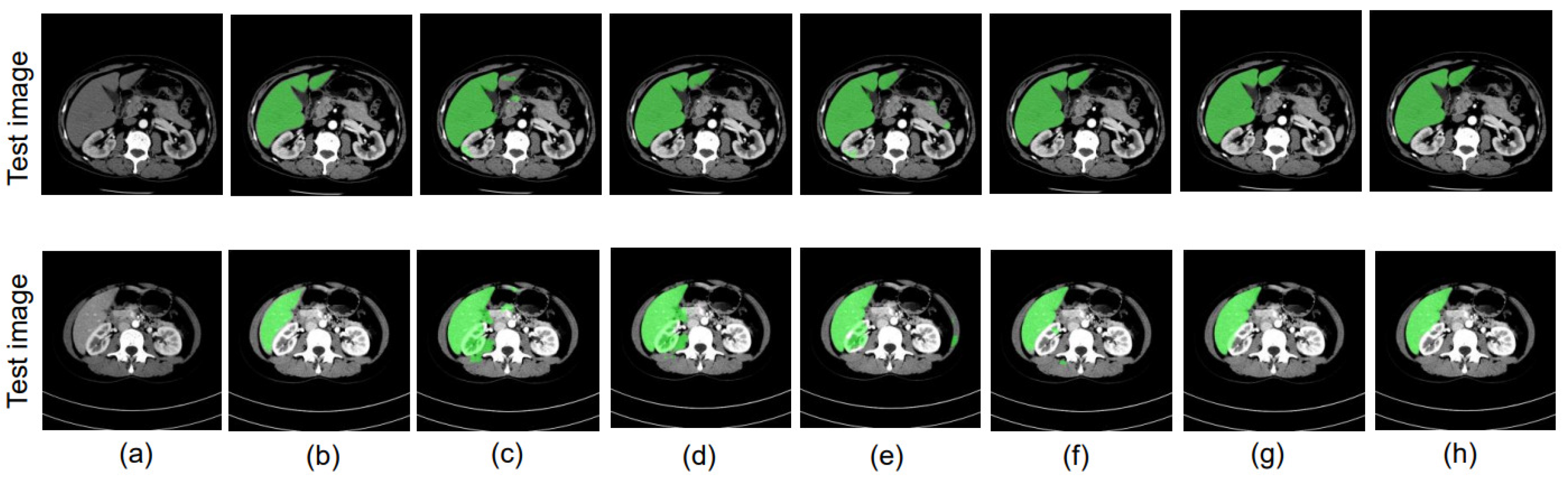
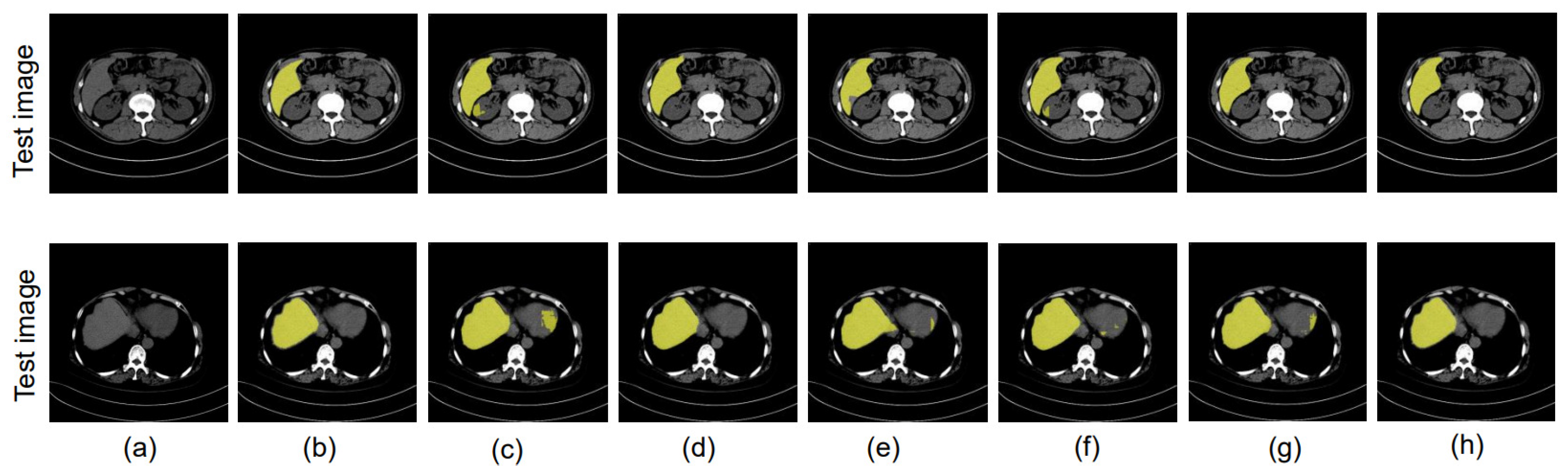
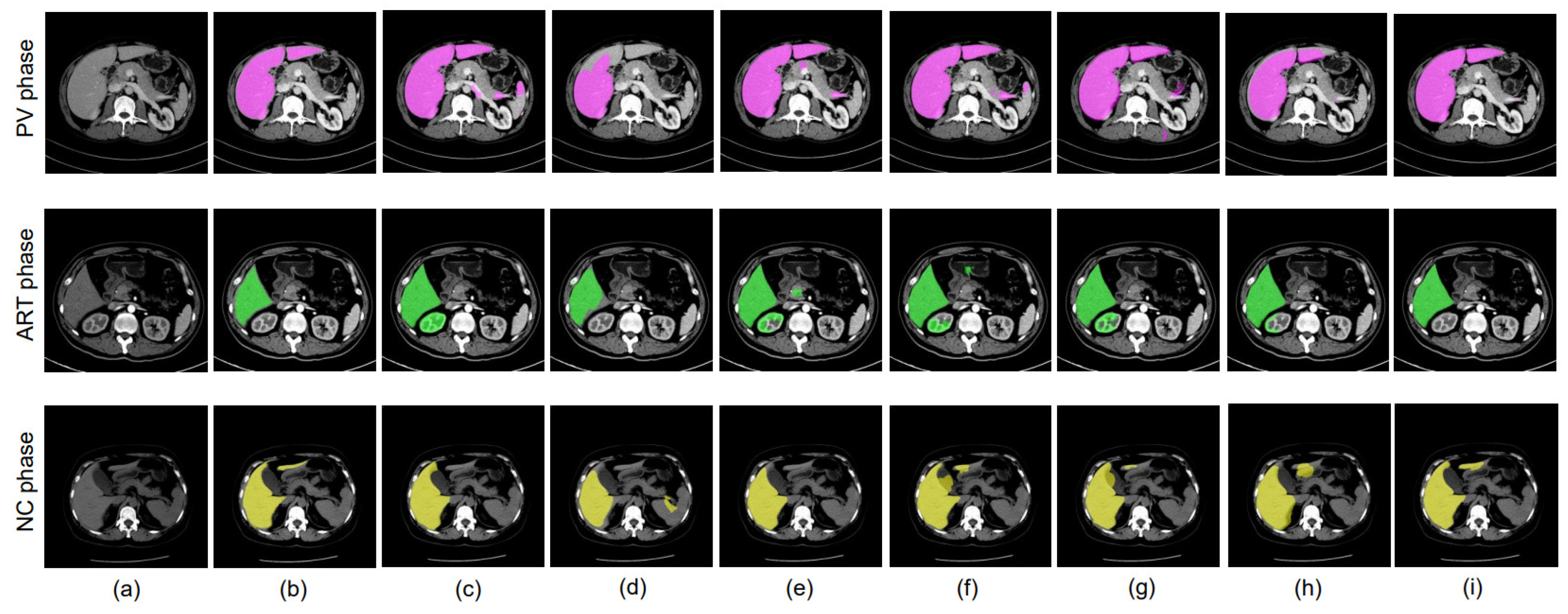
4. Results
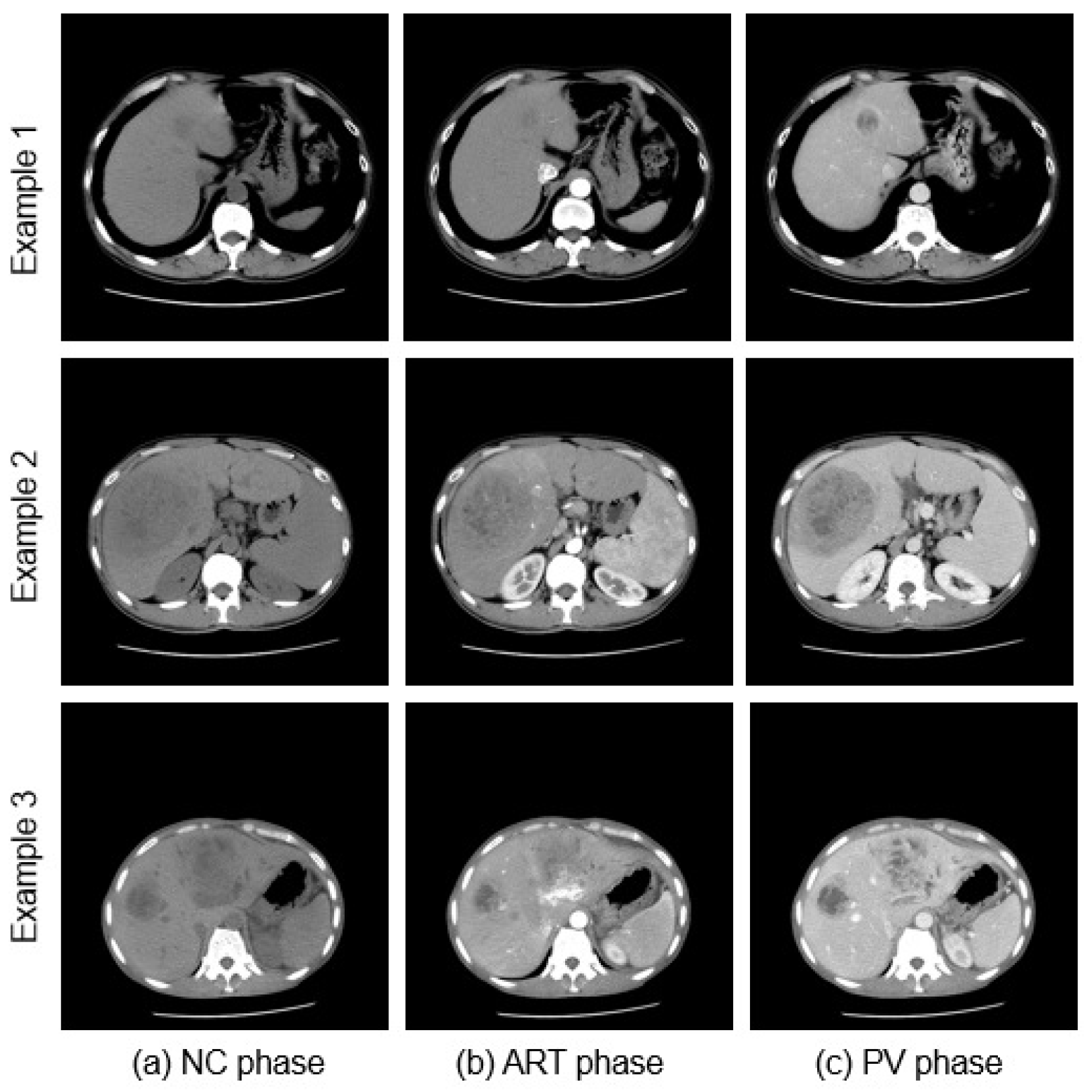
4.1. Dataset
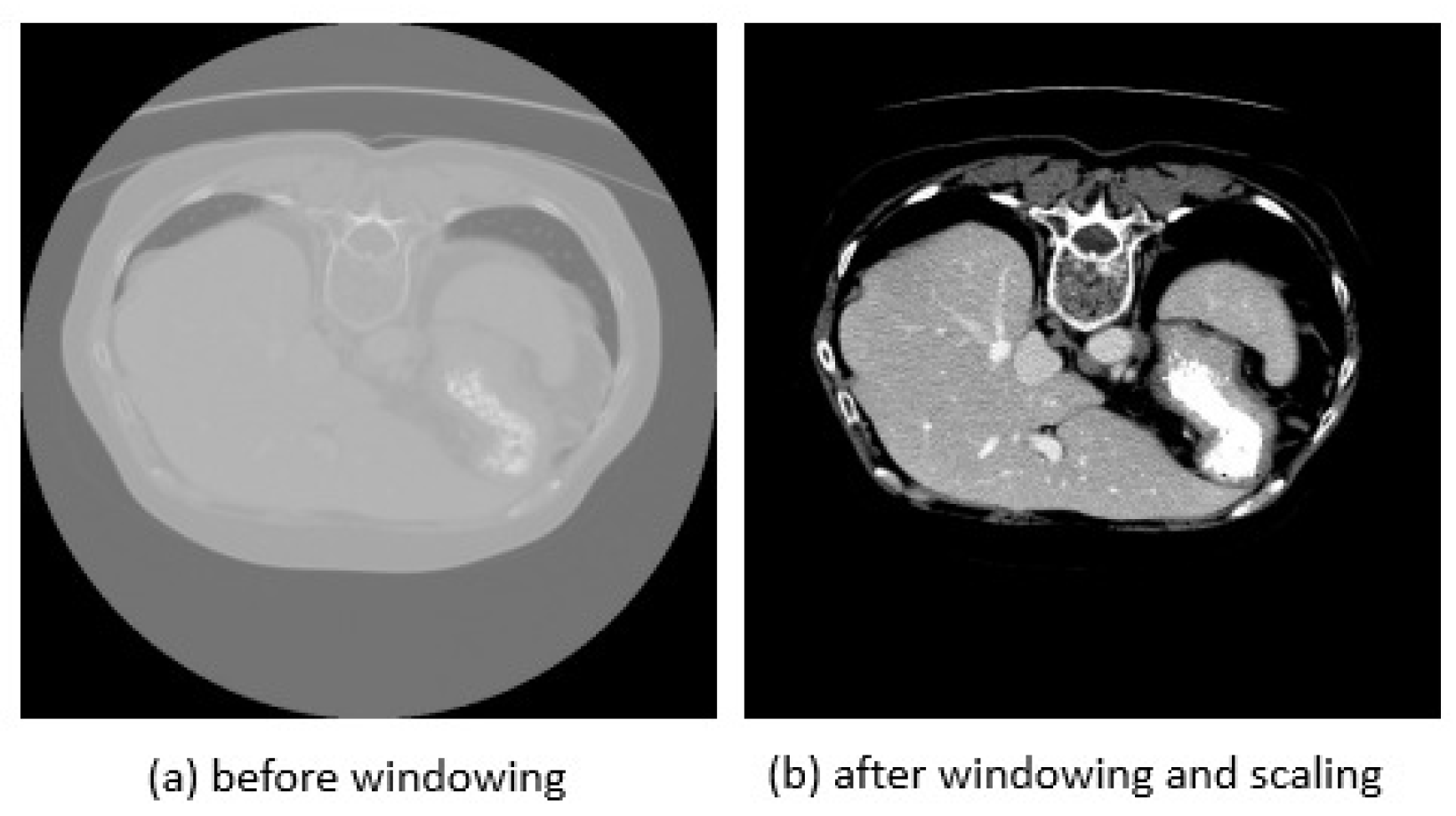
4.2. Data Preprocessing
4.3. Implementation Details
4.4. Training Strategy
4.5. Evaluation
4.5.1. Dice Coefficient (DC)/F1 Score
4.5.2. Intersection over Union (IoU)/Jaccard
4.5.3. Sensitivity/True Positive Rate (TRP)/Recall
4.5.4. Precision/Positive Predicted Value (PPV)
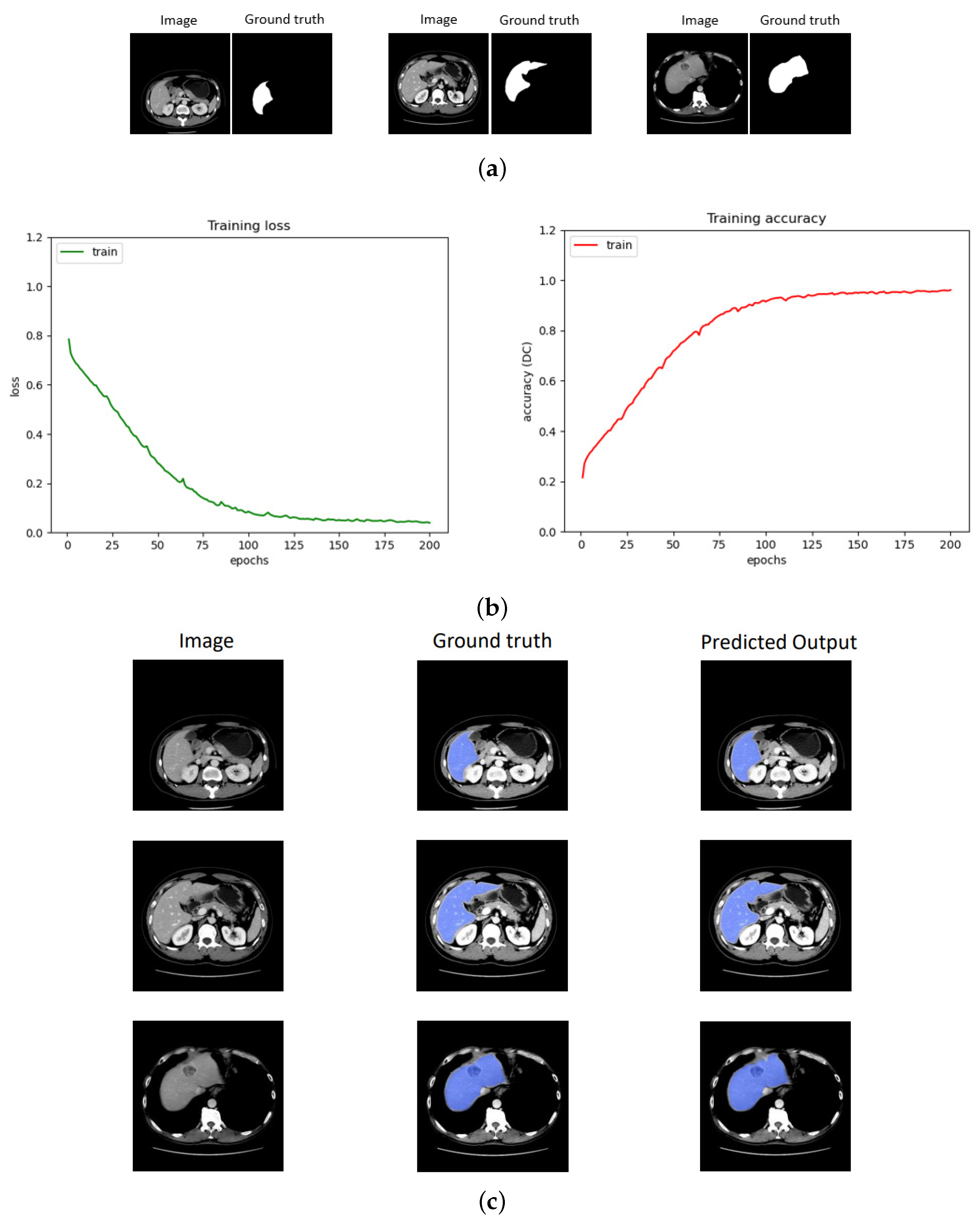
4.6. Performance Evaluation of the Training Model
4.7. Evaluation of Proposed DD-UDA Framework Based on Hyperparameters Such as Adversarial Weights

| Proposed DD-UDA | PV(LiTS)→ PV(MPCT-FLL) | PV(LiTS)→ ART(MPCT-FLL) | PV(LiTS)→ NC(MPCT-FLL) | ||
|---|---|---|---|---|---|
| DC | DC | DC | |||
| 0.0005 | 0.0005 | 0.885 | 0.887 | 0.855 | |
| 0.0005 | 0.003 | 0.894 | 0.888 | 0.872 | |
| 0.0005 | 0.007 | 0.872 | 0.866 | 0.845 |
4.8. Ablation Study
4.8.1. Different Datacenter and Same Phase
4.8.2. Same Datacenter and Different Phase
4.8.3. Different Datacenter and Different Phase
4.9. Evaluation of Proposed Methods with SegNet as the Backbone
4.10. Comparison with the State-of-the-Art Methods
5. Discussion
6. Conclusions
Author Contributions
Funding
Institutional Review Board Statement
Informed Consent Statement
Data Availability Statement
Conflicts of Interest
References
- Tang, W.; Zou, D.; Yang, S.; Shi, J.; Dan, J.; Song, G. A two-stage approach for automatic liver segmentation with Faster R-CNN and DeepLab. Neural Comput. Appl. 2020, 32, 6769–6778. [Google Scholar] [CrossRef]
- Yasaka, K.; Akai, H.; Abe, O.; Kiryu, S. Deep learning with convolutional neural network for differentiation of liver masses at dynamic contrast-enhanced CT: A preliminary study. Radiology 2018, 286, 887–896. [Google Scholar] [CrossRef] [PubMed] [Green Version]
- Campadelli, P.; Casiraghi, E.; Esposito, A. Liver segmentation from computed tomography scans: A survey and a new algorithm. Artif. Intell. Med. 2009, 45, 185–196. [Google Scholar] [CrossRef] [PubMed]
- Chen, Y.W.; Jain, L.C. (Eds.) Deep Learning in Healthcare; Springer: Berlin/Heidelberg, Germany, 2020. [Google Scholar]
- Ronneberger, O.; Fischer, P.; Brox, T. U-net: Convolutional networks for biomedical image segmentation. In International Conference on Medical Image Computing and Computer-Assisted Intervention; Springer: Cham, Switzerland, 2015; pp. 234–241. [Google Scholar]
- Long, J.; Shelhamer, E.; Darrell, T. Fully convolutional networks for semantic segmentation. In Proceedings of the IEEE Conference on Computer Vision and Pattern Recognition, Boston, MA, USA, 7–12 June 2015; pp. 3431–3440. [Google Scholar]
- Ben-Cohen, A.; Diamant, I.; Klang, E.; Amitai, M.; Greenspan, H. Fully convolutional network for liver segmentation and lesions detection. In Deep Learning and Data Labeling for Medical Applications; Springer: Cham, Switzerland, 2016; pp. 77–85. [Google Scholar]
- Huang, H.; Lin, L.; Tong, R.; Hu, H.; Zhang, Q.; Iwamoto, Y.; Han, X.; Chen, Y.W.; Wu, J. UNet 3+: A full-scale connected unet for medical image segmentation. In Proceedings of the ICASSP 2020—2020 IEEE International Conference on Acoustics, Speech and Signal Processing (ICASSP), Barcelona, Spain, 4–8 May 2020; pp. 1055–1059. [Google Scholar]
- Hasegawa, R.; Iwamoto, Y.; Han, X.; Lin, L.; Hu, H.; Cai, X.; Chen, Y.W. Automatic detection and segmentation of liver tumors in multi-phase ct images by phase attention mask r-cnn. In Proceedings of the IEEE International Conference on Consumer Electronics (ICCE), Las Vegas, NV, USA, 10–12 January 2021; pp. 1–5. [Google Scholar]
- Xu, Y.; Cai, M.; Lin, L.; Zhang, Y.; Hu, H.; Peng, Z.; Zhang, Q.; Chen, Q.; Mao, X.; Iwamoto, Y.; et al. PA-ResSeg: A phase attention residual network for liver tumor segmentation from multiphase CT images. Med. Phys. 2021, 48, 3752–3766. [Google Scholar] [CrossRef] [PubMed]
- Lee, S.; Kim, D.; Kim, N.; Jeong, S.G. Drop to adapt: Learning discriminative features for unsupervised domain adaptation. In Proceedings of the IEEE/CVF International Conference on Computer Vision, Seoul, Republic of Korea, 27 October–2 November 2019; pp. 91–100. [Google Scholar]
- Wang, M.; Deng, W. Deep visual domain adaptation: A survey. Neurocomputing 2018, 312, 135–153. [Google Scholar] [CrossRef] [Green Version]
- Shen, R.; Yao, J.; Yan, K.; Tian, K.; Jiang, C.; Zhou, K. Unsupervised domain adaptation with adversarial learning for mass detection in mammogram. Neurocomputing 2020, 393, 27–37. [Google Scholar] [CrossRef]
- Hoffman, J.; Wang, D.; Yu, F.; Darrell, T. Fcns in the wild: Pixel-level adversarial and constraint-based adaptation. arXiv 2016, arXiv:1612.02649. [Google Scholar]
- Tzeng, E.; Hoffman, J.; Zhang, N.; Saenko, K.; Darrell, T. Deep domain confusion: Maximizing for domain invariance. arXiv 2014, arXiv:1412.3474. [Google Scholar]
- Kanopoulos, N.; Vasanthavada, N.; Baker, R.L. Design of an image edge detection filter using the Sobel operator. IEEE J. Solid-State Circuits 1988, 23, 358–367. [Google Scholar] [CrossRef]
- Bilic, P.; Christ, P.; Li, H.B.; Vorontsov, E.; Ben-Cohen, A.; Kaissis, G.; Szeskin, A.; Jacobs, C.; Mamani, G.E.H.; Chartrand, G.; et al. The liver tumor segmentation benchmark (lits). arXiv 2019, arXiv:1901.04056. [Google Scholar] [CrossRef] [PubMed]
- Ananda, S.; Iwamoto, Y.; Han, X.; Lin, L.; Hu, H.; Chen, Y.W. Dual Discriminator-Based Unsupervised Domain Adaptation Using Adversarial Learning for Liver Segmentation on Multiphase CT Images. In Proceedings of the 44th Annual International Conference of the IEEE Engineering in Medicine & Biology Society (EMBC), Glasgow, UK, 11–15 July 2022; pp. 1552–1555. [Google Scholar]
- Zhou, Z.; Rahman Siddiquee, M.M.; Tajbakhsh, N.; Liang, J. Unet++: A nested u-net architecture for medical image segmentation. In Deep Learning in Medical Image Analysis and Multimodal Learning for Clinical Decision Support; Springer: Cham, Switzerland, 2018; pp. 3–11. [Google Scholar]
- Todoroki, Y.; Iwamoto, Y.; Lin, L.; Hu, H.; Chen, Y.W. Automatic detection of focal liver lesions in multi-phase CT images using a multi-channel & multi-scale CNN. In Proceedings of the International Conference of the IEEE Engineering in Medicine and Biology Society (EMBC), Berlin, Germany, 23–27 July 2019; pp. 872–875. [Google Scholar]
- Jinbo, H.; Kitrungrotsaku, T.; Iwamoto, Y.; Lin, L.; Hu, H.; Chen, Y.W. Development of an Interactive Semantic Medical Image Segmentation System. In Proceedings of the 9th Global Conference on Consumer Electronics (GCCE), Kobe, Japan, 13–16 October 2020; pp. 678–681. [Google Scholar]
- Huang, H.; Zheng, H.; Lin, L.; Cai, M.; Hu, H.; Zhang, Q.; Chen, Q.; Iwamoto, Y.; Han, X.; Chen, Y.W.; et al. Medical Image Segmentation with Deep Atlas Prior. IEEE Trans. Med. Imaging 2021, 40, 3519–3530. [Google Scholar] [CrossRef] [PubMed]
- Zhuang, F.; Cheng, X.; Luo, P.; Pan, S.J.; He, Q. Supervised representation learning: Transfer learning with deep autoencoders. In Proceedings of the Twenty-Fourth International Joint Conference on Artificial Intelligence, Buenos Aires, Argentina, 25–31 July 2015. [Google Scholar]
- Toldo, M.; Maracani, A.; Michieli, U.; Zanuttigh, P. Unsupervised domain adaptation in semantic segmentation: A review. Technologies 2020, 2, 35. [Google Scholar] [CrossRef]
- Tzeng, E.; Hoffman, J.; Saenko, K.; Darrell, T. Adversarial discriminative domain adaptation. In Proceedings of the IEEE Conference on Computer Vision and Pattern Recognition, Honolulu, HI, USA, 21–26 July 2017; pp. 7167–7176. [Google Scholar]
- Javanmardi, M.; Tolga, T. Domain adaptation for biomedical image segmentation using adversarial training. In Proceedings of the IEEE 15th International Symposium on Biomedical Imaging (ISBI), Washington, DC, USA, 4–7 April 2018; pp. 554–558. [Google Scholar]
- Panfilov, E.; Tiulpin, A.; Klein, S.; Nieminen, M.T.; Saarakkala, S. Improving robustness of deep learning based knee mri segmentation: Mixup and adversarial domain adaptation. In Proceedings of the IEEE/CVF International Conference on Computer Vision Workshops, Long Beach, CA, USA, 16–17 June 2019. [Google Scholar]
- Vu, T.H.; Jain, H.; Bucher, M.; Cord, M.; Pérez, P. Advent: Adversarial entropy minimization for domain adaptation in semantic segmentation. In Proceedings of the IEEE/CVF Conference on Computer Vision and Pattern Recognition, Long Beach, CA, USA, 15–20 June 2019; pp. 2517–2526. [Google Scholar]
- Chen, M.; Xue, H.; Cai, D. Domain adaptation for semantic segmentation with maximum squares loss. In Proceedings of the IEEE/CVF International Conference on Computer Vision, Seoul, Republic of Korea, 27 October–2 November 2019; pp. 2090–2099. [Google Scholar]
- Huang, X.; Lin, Z.; Jiao, Y.; Chan, M.T.; Huang, S.; Wang, L. Two-Stage segmentation framework based on distance transformation. Sensors 2022, 22, 250. [Google Scholar] [CrossRef] [PubMed]
- Maas, A.L.; Hannun, A.Y.; Ng, A.Y. Rectifier nonlinearities improve neural network acoustic models. In Proceedings of the 30th International Conference on Machine Learning, Atlanta, GA, USA, 16–21 June 2013. [Google Scholar]
- Kingma, D.P.; Ba, J. Adam: A method for stochastic optimization. arXiv 2014, arXiv:1412.6980. [Google Scholar]
- Badrinarayanan, V.; Kendall, A.; Cipolla, R. Segnet: A deep convolutional encoder-decoder architecture for image segmentation. IEEE Trans. Pattern Anal. Mach. Intell. 2017, 39, 2481–2495. [Google Scholar] [CrossRef] [PubMed]
- Jain, R.K.; Sato, T.; Watasue, T.; Nakagawa, T.; Iwamoto, Y.; Han, X.; Lin, L.; Hu, H.; Ruan, X.; Chen, Y.W. Unsupervised domain adaptation using adversarial learning and maximum square loss for liver tumors detection in multi-phase CT images. In Proceedings of the 44th Annual International Conference of the IEEE Engineering in Medicine & Biology Society (EMBC), Glasgow, UK, 11–15 July 2022; pp. 1536–1539. [Google Scholar]


| Method | Strength | Limitations |
|---|---|---|
| U-Net [5] | Can perform segmentation using smaller dataset. | Lower generalization capability when tested on unknown datasets. |
| UDA [13] | Adaptation is performed at output level using single discriminator. | This method does not show improved results for the PV and NC phases. |
| UDA(GRL) [26] | Adaptation is performed using GRL layer. | This method achieves better results only for the NC phase. |
| Advent [28] | Adaptation is performed by converting feature maps to entropy maps. | This approach show poor results on medical datasets. |
| MSL [29] | Adaptation is performed using the maximum square loss without discriminator. | This approach does not achieve better results for certain phases, and is designed for multi-class segmentation. |
| Proposed Method | Adaptation is carried out by employing two discriminators, one for each of the feature and output levels. We introduce an additional decoder to effectively learn the boundary features. | Our proposed method requires more trainable parameters. |
| Encoder | Decoder-1 and Decoder-2 | ||
|---|---|---|---|
| Layer | Details (Kernel Size, Output Channels, BN, Leaky Relu, Stride, Padding) | Layer | Details |
| input | CT image | upsample1 | upsample of conv5-2 concatenate with conv4-2 |
| conv1-1 | , BN, Leaky Relu, 2, 1 | conv 6-1 | Leaky Relu |
| conv1-2 | ,BN, Leaky Relu, 2, 1 | conv 6-2 | Leaky Relu |
| pool 1 | , 2 | upsample2 | upsample of conv6-2 concatenate with conv3-2 |
| conv2-1 | ,BN, Leaky Relu, 2, 1 | conv 7-1 | Leaky Relu |
| conv2-2 | ,BN, Leaky Relu, 2, 1 | conv 7-2 | Leaky Relu |
| pool 2 | , 2 | upsample3 | upsample of conv7-2 concatenate with conv2-2 |
| conv3-1 | ,BN, Leaky Relu, 2, 1 | conv 8-1 | Leaky Relu |
| conv3-2 | ,BN, Leaky Relu, 2, 1 | conv 8-2 | Leaky Relu |
| pool 3 | , 2 | upsample4 | upsample of conv8-2 concatenate with conv1-2 |
| conv4-1 | ,BN, Leaky Relu, 2, 1 | conv 9-1 | Leaky Relu |
| conv4-2 | ,BN, Leaky Relu, 2, 1 | conv 9-2 | Leaky Relu |
| pool 4 | , 2 | conv 10 | |
| conv5-1 | ,BN, Leaky Relu, 2, 1 | ||
| conv5-2 | ,BN, Leaky Relu, 2, 1 | ||
| Layers | Output | Operation, Kernel Size Output Channels, Stride |
|---|---|---|
| Layer-1 | Conv, , 64, 2 | |
| Layer-2 | Conv, , 128, 2 | |
| Layer-3 | Conv, , 256, 2 | |
| Layer-4 | Conv, , 512, 2 | |
| Layer-5 | Conv, , 1, 2 |
| PV(MPCT-FLL)→ART(MPCT-FLL) | PV(MPCT-FLL)→ NC(MPCT-FLL) | |||||
|---|---|---|---|---|---|---|
| Source | Target | Test | Source | Target | Test | |
| No. of Patients | 71 | 39 | 11 | 71 | 39 | 11 |
| No. of slices | 1888 | 985 | 257 | 1888 | 989 | 255 |
| PV(LiTS)→ PV(MPCT-FLL) | PV(LiTS)→ ART(MPCT-FLL) | PV(LiTS)→ NC(MPCT-FLL) | |||||||
|---|---|---|---|---|---|---|---|---|---|
| Source | Target | Test | Source | Target | Test | Source | Target | Test | |
| No. of Patients | 111 | 110 | 11 | 111 | 110 | 11 | 111 | 110 | 11 |
| No. of slices | 16,156 | 2887 | 274 | 16,156 | 2881 | 257 | 16,156 | 2855 | 255 |
| Method | Boundary | UDA | DD-UDA | PV(LiTS)→ PV(MPCT-FLL) | |||
|---|---|---|---|---|---|---|---|
| DC | IoU | TRP | PPV | ||||
| U-Net [5] | 0.866 | 0.775 | 0.549 | 0.788 | |||
| Proposed Boundary-enhanced U-Net | ✓ | 0.877 | 0.793 | 0.546 | 0.805 | ||
| U-Net+UDA (baseline) [13] | ✓ | 0.872 | 0.785 | 0.916 | 0.812 | ||
| Proposed Boundary- enhanced U-Net+UDA | ✓ | ✓ | 0.884 | 0.803 | 0.967 | 0.823 | |
| U-Net+ Proposed DD-UDA [18] | ✓ | 0.894 | 0.817 | 0.983 | 0.828 | ||
| Proposed Boundary- enhanced U-Net+ DD-UDA | ✓ | ✓ | 0.892 | 0.823 | 0.975 | 0.830 | |
| Method | Boundary | UDA | DD- UDA | PV(MPCT-FLL)→ ART(MPCT-FLL) | PV(MPCT-FLL)→ NC(MPCT-FLL) | ||||||
|---|---|---|---|---|---|---|---|---|---|---|---|
| DC | IoU | TRP | PPV | DC | IoU | TRP | PPV | ||||
| U-Net [5] | 0.905 | 0.846 | 0.543 | 0.903 | 0.859 | 0.785 | 0.544 | 0.863 | |||
| Proposed Boundary -enhanced U-Net | ✓ | 0.913 | 0.853 | 0.572 | 0.908 | 0.862 | 0.788 | 0.584 | 0.865 | ||
| U-Net+UDA (baseline) [13] | ✓ | 0.914 | 0.859 | 0.878 | 0.919 | 0.893 | 0.829 | 0.847 | 0.895 | ||
| Proposed Boundary- enhanced U-Net+UDA | ✓ | ✓ | 0.918 | 0.872 | 0.844 | 0.924 | 0.894 | 0.852 | 0.836 | 0.852 | |
| U-Net+ Proposed DD-UDA [18] | ✓ | 0.921 | 0.863 | 0.875 | 0.922 | 0.911 | 0.857 | 0.902 | 0.903 | ||
| Proposed Boundary- enhanced U-Net+DD-UDA | ✓ | ✓ | 0.922 | 0.883 | 0.929 | 0.934 | 0.912 | 0.862 | 0.897 | 0.924 | |
| Method | Boundary | UDA | DD- UDA | PV(LiTS)→ ART(MPCT-FLL) | PV(LiTS)→ NC(MPCT-FLL) | ||||||
|---|---|---|---|---|---|---|---|---|---|---|---|
| DC | IoU | TRP | PPV | DC | IoU | TRP | PPV | ||||
| U-Net [5] | 0.826 | 0.728 | 0.560 | 0.752 | 0.825 | 0.736 | 0.564 | 0.741 | |||
| Proposed Boundary- enhanced U-Net | ✓ | 0.844 | 0.753 | 0.537 | 0.537 | 0.779 | 0.749 | 0.535 | 0.762 | ||
| U-Net+UDA (baseline) [13] | ✓ | 0.880 | 0.796 | 0.966 | 0.813 | 0.855 | 0.772 | 0.944 | 0.811 | ||
| Proposed Boundary- enhanced U-Net+UDA | ✓ | ✓ | 0.874 | 0.789 | 0.892 | 0.821 | 0.864 | 0.781 | 0.818 | 0.811 | |
| U-Net+Proposed DD-UDA [18] | ✓ | 0.888 | 0.808 | 0.750 | 0.832 | 0.872 | 0.794 | 0.662 | 0.821 | ||
| Proposed Boundary- enhanced U-Net+ DD-UDA | ✓ | ✓ | 0.890 | 0.811 | 0.966 | 0.838 | 0.875 | 0.800 | 0.945 | 0.832 | |
| Method | PV(LiTS)→ PV(MPCT-FLL) | PV(LiTS)→ ART(MPCT-FLL) | PV(LiTS)→ NC(MPCT-FLL) | |||||||||
|---|---|---|---|---|---|---|---|---|---|---|---|---|
| DC | IoU | TRP | PPV | DC | IoU | TRP | PPV | DC | IoU | TRP | PPV | |
| SegNet [33] | 0.879 | 0.796 | 0.747 | 0.819 | 0.868 | 0.783 | 0.667 | 0.809 | 0.836 | 0.750 | 0.632 | 0.802 |
| Proposed Boundary -enhanced SegNet | 0.884 | 0.805 | 0.825 | 0.826 | 0.861 | 0.779 | 0.738 | 0.822 | 0.845 | 0.762 | 0.681 | 0.808 |
| SegNet+Proposed DD-UDA [18] | 0.890 | 0.813 | 0.893 | 0.830 | 0.896 | 0.819 | 0.966 | 0.838 | 0.886 | 0.811 | 0.850 | 0.841 |
| Proposed Boundary- enhanced SegNet+ DD-UDA | 0.901 | 0.828 | 0.929 | 0.850 | 0.899 | 0.823 | 0.959 | 0.843 | 0.894 | 0.822 | 0.933 | 0.840 |
| Method | PV(LiTS)→ PV(MPCT-FLL) | PV(LiTS)→ ART(MPCT-FLL) | PV(LiTS)→ NC(MPCT-FLL) | |||||||||
|---|---|---|---|---|---|---|---|---|---|---|---|---|
| DC | IoU | TRP | PPV | DC | IoU | TRP | PPV | DC | IoU | TRP | PPV | |
| No adaptation | ||||||||||||
| U-Net [5] | 0.866 | 0.775 | 0.549 | 0.788 | 0.826 | 0.728 | 0.560 | 0.752 | 0.825 | 0.736 | 0.564 | 0.741 |
| U-Net 3+ [8] | 0.878 | 0.794 | 0.976 | 0.809 | 0.869 | 0.781 | 0.960 | 0.802 | 0.847 | 0.758 | 0.938 | 0.791 |
| Unsupervised domain adaptation | ||||||||||||
| UDA [13] | 0.872 | 0.785 | 0.916 | 0.812 | 0.880 | 0.796 | 0.966 | 0.813 | 0.855 | 0.772 | 0.944 | 0.811 |
| ADVENT [28] | 0.706 | 0.629 | 0.500 | 0.706 | 0.629 | 0.547 | 0.500 | 0.668 | 0.626 | 0.538 | 0.500 | 0.664 |
| MSL+IW [29] | 0.884 | 0.803 | 0.978 | 0.818 | 0.863 | 0.777 | 0.963 | 0.797 | 0.833 | 0.747 | 0.952 | 0.813 |
| UDA(GRL) [26] | 0.879 | 0.796 | 0.981 | 0.807 | 0.853 | 0.769 | 0.935 | 0.810 | 0.863 | 0.787 | 0.929 | 0.826 |
| UDA(MIXUP) [27] | 0.870 | 0.784 | 0.613 | 0.812 | 0.880 | 0.797 | 0.960 | 0.816 | 0.854 | 0.766 | 0.958 | 0.781 |
| UDA+MSL [34] | 0.874 | 0.790 | 0.500 | 0.827 | 0.863 | 0.782 | 0.804 | 0.808 | 0.834 | 0.751 | 0.909 | 0.810 |
| Proposed DD-UDA [18] | 0.894 | 0.817 | 0.983 | 0.828 | 0.888 | 0.808 | 0.750 | 0.832 | 0.872 | 0.794 | 0.662 | 0.821 |
| Proposed Boundary- enhanced U-Net+DD-UDA | 0.892 | 0.823 | 0.975 | 0.830 | 0.890 | 0.811 | 0.966 | 0.838 | 0.875 | 0.800 | 0.945 | 0.832 |
Disclaimer/Publisher’s Note: The statements, opinions and data contained in all publications are solely those of the individual author(s) and contributor(s) and not of MDPI and/or the editor(s). MDPI and/or the editor(s) disclaim responsibility for any injury to people or property resulting from any ideas, methods, instructions or products referred to in the content. |
© 2023 by the authors. Licensee MDPI, Basel, Switzerland. This article is an open access article distributed under the terms and conditions of the Creative Commons Attribution (CC BY) license (https://creativecommons.org/licenses/by/4.0/).
Share and Cite
Ananda, S.; Jain, R.K.; Li, Y.; Iwamoto, Y.; Han, X.-H.; Kanasaki, S.; Hu, H.; Chen, Y.-W. A Boundary-Enhanced Liver Segmentation Network for Multi-Phase CT Images with Unsupervised Domain Adaptation. Bioengineering 2023, 10, 899. https://doi.org/10.3390/bioengineering10080899
Ananda S, Jain RK, Li Y, Iwamoto Y, Han X-H, Kanasaki S, Hu H, Chen Y-W. A Boundary-Enhanced Liver Segmentation Network for Multi-Phase CT Images with Unsupervised Domain Adaptation. Bioengineering. 2023; 10(8):899. https://doi.org/10.3390/bioengineering10080899
Chicago/Turabian StyleAnanda, Swathi, Rahul Kumar Jain, Yinhao Li, Yutaro Iwamoto, Xian-Hua Han, Shuzo Kanasaki, Hongjie Hu, and Yen-Wei Chen. 2023. "A Boundary-Enhanced Liver Segmentation Network for Multi-Phase CT Images with Unsupervised Domain Adaptation" Bioengineering 10, no. 8: 899. https://doi.org/10.3390/bioengineering10080899