Article

EnviroStream: A Stream Reasoning Benchmark for Environmental and Climate Monitoring

by
Elena Mastria
1,†,
Francesco Pacenza
1,†,
Jessica Zangari
1,†,
Francesco Calimeri
1,2,‡,
Simona Perri
1,‡ and
Giorgio Terracina
1,*,‡
1
Department of Mathematics and Computer Science, University of Calabria, 87036 Rende, Italy
2
DLVSystem Ltd., Via della Resistenza 19/C, 87036 Rende, Italy
*
Author to whom correspondence should be addressed.
These authors contributed equally to this work.
Big Data Cogn. Comput. 2023, 7(3), 135; https://doi.org/10.3390/bdcc7030135
Submission received: 2 May 2023 / Revised: 20 July 2023 / Accepted: 25 July 2023 / Published: 31 July 2023
(This article belongs to the Special Issue Big Data and Cognitive Computing in 2023)

Abstract

:
Stream Reasoning (SR) focuses on developing advanced approaches for applying inference to dynamic data streams; it has become increasingly relevant in various application scenarios such as IoT, Smart Cities, Emergency Management, and Healthcare, despite being a relatively new field of research. The current lack of standardized formalisms and benchmarks has been hindering the comparison between different SR approaches. We proposed a new benchmark, called EnviroStream, for evaluating SR systems on weather and environmental data. The benchmark includes queries and datasets of different sizes. We adopted I-DLV-sr, a recently released SR system based on Answer Set Programming, as a baseline for query modelling and experimentation. We also showcased continuous online reasoning via a web application.

1. Introduction

Stream Reasoning (SR) [1,2] is a relatively new field of research that has evolved from Stream Processing (SP). It focuses on studying and developing advanced approaches and techniques for continuously applying inference to highly dynamic data streams. These theoretically infinite streams of data change over time, generated by sources such as sensors, devices, and social networks that monitor physical or virtual environments and report on their status and changes. While SP aims to quickly process data streams and answer continuous queries on their elements, SR tackles the challenge of inferring new information based on both the elements in the data streams and background knowledge on the application domain. Recently, SR has been studied in depth, far beyond the academic context, and has therefore become increasingly relevant in various application scenarios, such as IoT, smart cities, emergency management, and healthcare. In such contexts, practical applications require the response to complex queries in very short time frames, defined according to the application domain in hand and typically in real or near real-time. Therefore, an SR system (i.e., a stream reasoner) must be able to efficiently perform continuous complex reasoning tasks while processing heterogeneous data streams together, and according to large background knowledge bases.
Over the past few years, different approaches to SR have been proposed, based on Complex Event Processing (CEP), Semantic Web or Knowledge Representation and Reasoning (KRR) [3,4,5,6]. However, to date, there are no standardized formalisms nor techniques for SR; this complicates the comparison between different approaches that are based on different languages, semantics and technologies. Indeed, even SR competitions are currently more oriented towards “model and solve” challenges rather than performance assessment [7]. Another crucial aspect for the advancement of the state-of-the-art is the availability of suitable benchmarks. Some first proposals can be found in the literature, concerning, e.g., social networks [8], an extended LUBM version [9], smart cities [10], social media [11], maritime traffic monitoring [12], and automobile traffic and autonomous driving [7]. However, only a few datasets include real data extracted from real-world domains. Moreover, there is an evident lack of benchmarks for logic-programming-based Stream Reasoning systems, as emerged in the recent Hackathon event [7].
Summarizing, the main desiderata for improving the current SR benchmark scenario can be outlined as follows: (i) provide proper means to simplify correctness checking; (ii) improve variety of supported input data formats; (iii) allow for the generation and customization of benchmark scenarios (scalability); (iv) increase availability of benchmarks for logic-based SR approaches.
In particular, desiderata (i) and (ii) attack both diversification of technologies and lack of standards. Desideratum (ii) fosters consumer agnosticism, whereas desideratum (iii) aims to overcome the limitations of fixed benchmarks that do not fit certain specificities of SR contexts, which require testing not only on the quantity of data but also on different time frames and the frequency of incoming data. Finally, desideratum (iv) tries to support the emerging area of research on logic-based SR systems.
The objective of the present work is to contribute precisely to the above desiderata. To this aim, we proposed EnviroStream, a novel benchmark for evaluating Stream Reasoning systems using weather and environmental data from European cities (names of the cities are omitted for anonymity reasons) including queries of interest in typical smart cities scenarios, such as monitoring air quality, noise pollution, heatwaves, rain intensity, and wind force. The queries were developed based on recommendations from organizations focused on human health and climate change.
In order to address desideratum (i), we provide both query definitions in textual format and their implementation in a logic-based language we recently proposed, which is supported by an actual system, namely I-DLV-sr  [13], as a baseline; in this way, any user of the benchmark can compare their results against the baseline. In order to improve data variety (desideratum (ii)), the benchmark data are provided in different formats, namely Datalog/ASP, plain JSON, and CSV. Moreover, we also intended to provide data in the RDF format in the next releases. Desideratum (iii) is tackled from several perspectives: besides providing different, ready to use, fixed datasets arranged in different sizes and time frames, we also provided an ad-hoc data generator which arranges the available data based on user-defined parameters allowing for arbitrary scaling and configuration of streaming data [7,11]; in this way, different aspects of any SR system can be tested. It is worth noting that benchmark data come from a real-world sensor network that is currently in use and growing, and they are continuously ingested; this allows us to periodically update the benchmark both with fresh data from existing sources and new data coming from additional measuring stations that will be available over time. Finally, the availability of data in the Datalog/ASP format along with a full-fledged logic-based SR system are clearly geared towards desideratum (iv).
Three datasets of different sizes (composed as described in Section 2.3) are publicly available on Zenodo (https://doi.org/10.5281/zenodo.8142369 (accessed on 1 May 2023)). In addition, the datasets, all queries modelled in the I-DLV-sr language along with instructions to run them, and a generator allowing the filtering of data on the basis of time frame and frequency, are reported in a dedicated GitHub repository https://github.com/DeMaCS-UNICAL/EnviroStream (accessed on 1 May 2023).
As a further contribution, we released a publicly accessible web site showcasing the online real-time reasoning performed by I-DLV-sr in the featured scenario; the application is available at https://experiments.demacs.unical.it (accessed on 1 May 2023).
The remainder of the paper is structured as follows. Section 2 describes EnviroStream data and queries. Section 3 illustrates how queries of EnviroStream can be modeled in the Stream Reasoning language of I-DLV-sr. Section 4 reports on the performance of I-DLV-sr when tested on EnviroStream. The web application is introduced in Section 5. Finally, Section 6 provides a final discussion and outlines future directions.

2. The EnviroStream Benchmark

In this section, we introduce and describe EnviroStream, a novel resource for benchmarking modern Stream Reasoning systems and applications that provides data and (continuous) reasoning tasks, both coming from real-world scenarios. We first illustrate the main features of EnviroStream, and discuss how it is placed in the context of related benchmarks; we then provide a thorough description of the benchmark, by both presenting the featured data and detailing all queries.

2.1. Main Features

As already mentioned, the benchmark features both data and reasoning tasks. The main features of EnviroStream, to date, can be summarized as follows:
Reasoning tasks are described by 10 queries, that:
require to manage time-based windows of varying size;
require to explicitly reason over time;
require to express various forms of aggregation across time slots and windows;
are supposed to be continuously processed over streams;
are both expressed in natural language and formally translated into a logic-based language for stream reasoning;
thanks to the translation and the availability of an actual system they come with proper means for correctness checking and baseline comparison.
Currently, the available data are streamed from weather sensors installed in European cities, and are such that:
they are continuously injected in real-time;
they are periodically incrementally updated and made available, thus fostering scalability, variety and continuous maintenance of data;
they are available in different formats, in order to foster the applicability of the benchmark also to different contexts, and grant consumer agnosticism [7];
besides static datasets, EnviroStream comes with a generator for tuning streams, thus allowing custom testing scenarios.

2.2. EnviroStream in the Context of SR Benchmarks

In the following, we describe how EnviroStream is placed in the context of the current related benchmarks. It is worth noting that, as a matter of fact, existing stream reasoning benchmarks mainly focus on RDF Stream Processing (RSP) and are geared towards continuous query answering under RDFS entailment regime [11]. Among these, one of the most popular is CityBench [10], which is also the closest to EnviroStream in terms of domain, being focused on smart cities. However, the two benchmarks significantly differ in the nature of the queries: EnviroStream requires an intensive use of time-based windows, thus explicitly stressing the evaluation capabilities of a tested SR system, whereas this aspect is covered by CityBench only to a limited extent. Indeed, in EnviroStream, windows are featured over all queries, with varying size spotlighting varying sections of the timeline. Other differences concern the nature of the data; while EnviroStream focuses on real data only, that are also continuously growing and updated, the CityBench dataset is static and hybrid, i.e., it features partly synthetic and partly real data. As for the data formats, beside those available in CityBench, EnviroStream also provides the Datalog/ASP one.
Coming to benchmark explicitly focused on SR based on logic programming, only two significant contributions are currently available. The first is the Maritime Monitoring benchmark [12]—it emerged from a real-world application and presents a relevant contribution featuring a large amount of real data; nevertheless, data are provided only in CSV format, with no means for scaling it. As already pointed out, in EnviroStream, not only are the real data provided in a number of different formats (thus increasing the already mentioned consumer agnosticism), but it also complies with one of the main desiderata for an SR benchmark: scalability. Indeed, thanks to an ad-hoc data generator, it allows for the arbitrary scaling and configuration of streaming data to be used [7,11]; this allows different aspects of the chosen system(s) to be tested.
The second contribution in the LP field, namely the Stream Reasoning Playground [7], has been released on the occasion of the Stream Reasoning Hackathon 2021  (https://streamreasoning.org/events/stream-reasoning-hackathon-2021/ (accessed on 1 May 2023)). The contribution is significant, as it incorporates the experience and the discussions from the hackaton. However, it is not conceived as a benchmark; rather, it is actually an extensible platform for data stream generation and pluggable data formatters. Notably, the platform features two scenarios, namely Traffic Monitoring and Autonomous Driving, that can be considered as the most relevant benchmarks for the logic-programming targets to date. EnviroStream is aimed at contributing to increasing the availability of resources for Stream Reasoning approaches and solutions based on logic-programming; it is worth noting that it shares with these benchmarks several points that make them both grant some desirable features in terms of widening targeted systems and data formats; in this respect, this testifies to the relevance of our proposal. In addition, EnviroStream further enriches the set of available data formats and introduces data that are continuously updated over time.

2.3. Data

The data include weather and environmental data from two European cities, whose names are omitted for anonymity reasons. Data are collected through weather stations scattered in each city. Each city has a station, which provides, approximately every 5 min, the following measures:
  • wind speed in m/s (meters per second);
  • wind direction in degrees;
  • relative humidity percentage;
  • external temperature in C (Celsius degrees);
  • noise in dB(A) (A—weighted decibels);
  • PM 2.5 , i.e., concentration of particulate matter of diameter 2.5 in μ g/m 3 (micro-grams per cubic meter of air);
  • PM 10 , i.e., concentration of particulate matter of diameter 10 in μ g/m 3 ;
  • atmospheric pressure in Kpa (Kilo-pascal);
  • optical rainfall in mm (millimeters).
Each station transmits the measures along with the associated measuring timestamps to a MongoDB (https://www.mongodb.com (accessed on 1 May 2023)) database, in charge of storing all of them. It is worth noting that stations send data separately, thus their measuring timestamps are not synchronized. Approximately, the database receives a bunch of data every 2 min. We provide three datasets of different sizes, freely available at https://doi.org/10.5281/zenodo.8142369 (accessed on 1 May 2023): day, night and large. day is a three hour dataset on a Wednesday afternoon (15 March 2023 from 12:00 p.m. to 03:00 p.m.), night is a three hour dataset on a Saturday night (from 11 March 2023 10:00 p.m. to 12 March 2023 01:00 a.m.) and large is a bigger dataset featuring detections from 1 January 2023 12:00 a.m. to 28 March 2023 11:59 p.m. Besides these static datasets, we provide a flexible generator allowing the filtering of data, configuring both data frequency and time frame and specifying the start and end points. Filtered data can be used to populate a MongoDB database or can be outputted via a TCP socket or standard output.

2.4. Queries

The queries focus on some crucial ambient topics: air quality, noise pollution, heatwave, rain intensity, and wind force. Studying the recommendations of major organizations promoting human health and monitoring climate change, we designed 2 queries for each topic.

2.4.1. Air Quality

The concentration of particulate matter has a high influence on human health as well as on the environment. Queries 1 and 2 focus on monitoring the concentration of PM 10 and PM 2.5 .
Query 1
Determination of the average of PM 10 and PM 2.5 measurements in the last 10 min and raise an alert if the PM 10 average is greater than or equal to 50 and/or the PM 2.5 average is greater than or equal to 25. The thresholds refer to the current European recommendation (https://environment.ec.europa.eu/topics/air/air-quality/eu-air-quality-standards_en (accessed on 1 May 2023)). The more the concentration of particulate matter in the air exceed these thresholds, the greater the health risks.
Query 2
Determination of the cities in which the PM 10 and PM 2.5 averages are maximum.

2.4.2. Noise Pollution

Noise pollution has been proven to have a crucial impact on human health, e.g., it contributes to cardiovascular effects and increases the incidence of coronary artery disease. Queries 3 and 4 focus on monitoring the noise exposure.
Query 3
Determination of the number of noise measurements exceeding the threshold recommended by the World Health Organisation (WHO) in the last hour. The WHO generally defines 65 dB(A) as the threshold during the day (from 6 a.m. to 10 p.m.) and 55 dB(A) at night (from 10 p.m. to 6 p.m.) (https://www.who.int/europe/news-room/fact-sheets/item/noise (accessed on 1 May 2023)).
Query 4
Determination of the cities in which a noise above 85 dB(A) was observed continuously for one hour. In fact, the WHO recommends that noise exposure should not exceed 85 dB(A) within an hour to avoid hearing impairment (https://apps.who.int/iris/bitstream/handle/10665/39458/9241540729-eng.pdf (accessed on 1 May 2023)).

2.4.3. Heat

Extreme heat can pose a health risk to the population. For instance, heat waves can occur when there are very high temperatures, often associated with high humidity, strong solar radiation and lack of ventilation. Humidex is one of the indices used to evaluate human climatic well-being in relation to humidity and temperature (https://www.canada.ca/en/environment-climate-change/services/seasonal-weather-hazards/warm-season-weather-hazards.html#toc7 (accessed on 1 May 2023)). It can be computed on the basis the temperature T and the relative humidity R (https://www.canada.ca/en/environment-climate-change/services/climate-change/canadian-centre-climate-services/display-download/technical-documentation-climate-normals.html (accessed on 1 May 2023)) as
humidex = T + h ,
where:
h = 0.5555 × ( e 10.0 ) e = 6.11 × e x p 5417.7530 × 1 273.15 1 d d = T 100 R 5
and ranges from 1 (little discomfort) to 4 (dangerous, possible heat stroke). Queries 5 and 6 monitor the Humidex to intercept extreme heat conditions.
Query 5
Alert when the Humidex is currently greater than 2 and has been above 2 at least 3 times in the last 30 min.
Query 6
Determination of the cities in which the Humidex results are always above 2 in the last 30 min.

2.4.4. Rain Intensity

Queries 7 and 8 regard rain monitoring, crucial to assess hydro-geological risks and droughts.
Query 7
Monitoring of the total millimeters of rain in the last hour and the classification of the rain intensity as light, moderate, or heavy. Rain is considered light if less than 25 mm fell in one hour, moderate if more than 25 mm and less than 76 mm fell in one hour, heavy if more than 76 mm fell in one hour (https://glossary.ametsoc.org/wiki/Rain (accessed on 1 May 2023)).
Query 8
Identification of the least rainy cities, i.e., those in which less millimeters of rain fell in the last hour.

2.4.5. Wind Force

Similar to rain, wind represents an atmospheric agent whose monitoring is essential for several aspects, including, e.g., wind energy, maritime conditions, or storm forecasts. The Beaufort scale is one of the most widely adopted systems for classifying wind force into 12 levels, ranging from calm wind to hurricane [14]. Queries 9 and 10 monitor the wind force, both using the Beaufort scale.
Query 9
Alert when the Beaufort level computed over the average wind speed in the last 10 min is above 6.
Query 10
Suppose L represents the current Beaufort level, this query determines, for each city, the duration in minutes for which the level has remained at L.

3. Modelling EnviroStream via the I-DLV-sr Language

In this section, we show how queries of EnviroStream can be modeled in an SR language.
As previously pointed out, in order to provide a formal baseline for the correctness checking of queries, we next provide the implementation of the 10 benchmark queries in a logic-based language we recently proposed, which is also supported by an actual system, namely I-DLV-sr  [13]. This formalization, along with their execution with I-DLV-sr, can be exploited by benchmark users to compare their results against the baseline.
The choice of I-DLV-sr is motivated by the fact that it has been designed to leverage state-of-the-art Stream Processing and Answer Set Programming (ASP) [15,16,17] technologies; I-DLV-sr is based on the integration of a custom Apache Flink application, ensuring a distributed processing of data streams, and the incremental version of the ASP system DLV2 [18], granting a continuous and incremental reasoning over time [19].
Before illustrating how EnviroStream queries have been modelled, we briefly recall I-DLV-sr input language via a high-level overview of its features. We suppose the reader to be familiar with basic concepts of ASP; for a comprehensive formal description of syntax, semantics, and properties of I-DLV-sr, we refer to  [13].

3.1. The I-DLV-sr Language

The language of I-DLV-sr consists in the ASP fragment of normal and stratified with respect to negation programs, extended with streaming literals and time-based constructs for enabling continuous online reasoning over data streams. In particular, the language includes different types of streaming literals based on four different operators: always, at least, at most and count. Their semantics is evaluated according to a stream  Σ , which is basically a sequence of sets of atoms Σ = S 0 , , S n . Each set is associated with a time point, i.e., a specific moment in time. An example of stream is depicted in Figure 1 in which, e.g., the atom b(5) is true in the time points 12 and 15.
Let us consider the stream Σ 1 as reported in Figure 1, and let us assume it to be at the 15-th time point (i.e., the current time point is 15). Table 1 reports some examples of ground (i.e., variable-free) streaming literals and specifies whether each of them holds according to Σ 1 at the current time point. The expression [2 sec] encompasses the last 2 s, i.e., it refers to the window consisting of the time points 13, 14 and 15. The expression {0,2}, instead, refers to the specific time points 15 and 13 (i.e., 0 and 2 s before the current time point, respectively). Note that the expression {0,1,2} is equivalent to [2 sec].
The always operator can be used to check that an atom holds in all considered time points: for instance, a(3) is always true in the window of the last two seconds. The count operator checks the occurrences of an atom in all the specified time points: e.g., b(5) occurs only once in the window of the last two seconds. Similarly, at least (resp., at most) checks that the number of occurrences is equal to or greater than (resp., less than) a given number. For instance, in the window consisting of the last two seconds, b(5) is true once: thus, we have both at least 1 and at most 1 occurrences of b(5).
A rule can have a predicate atom (defined as in the ASP-Core-2 standard) in the head and a conjunction of literals in the body. The body may contain streaming literals, all types of literals defined in the ASP-Core-2 standard such as aggregates, as well as external literals whose semantics can be defined externally via custom Python3 functions. A program is a finite set of rules, and has to be stratified according to the definition given in [13].
As an example, the following is an I-DLV-sr program:
                      c(Z) :- b(X), a(X), &sum(X,Y;Z). d(X) :- c(X) at least 1 in [1 sec].
where c(Z), b(X), a(X), and d(X) are predicate atoms, c(X) at least 1 in [1 sec] is a streaming literal, and &sum(X,Y;Z) is an external literal, whose meaning could be, for instance, defined via the following Python function:
def 
sum(a, b):
return a+b
Furthermore, the language features a dedicated construct for explicitly dealing with time, namely the @now construct; it is a special form of term that, at each time point t, is automatically assigned with the value of t. @now can be either (1) numeric, i.e., an integer number representing t in seconds, minutes or hours or (2) textual, i.e., a string in the datetime format: yyyy-MM-ddTHH:mm:ss.SSS. In case (2), one can also access a specific field via the “dot notation” (e.g., @now.hour). For instance, let us refer to the example stream Σ 1 introduced above, and let us assume (again) to be at time point 15; then, the rule:
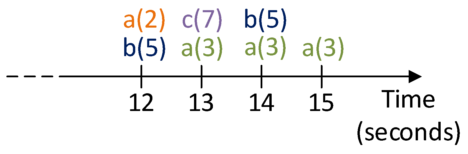
                      occurring_time_a(X,Y) :- a(X,@now).
allows one to infer occurring_time_a(3,15).
Finally, it is worth pointing out that, as far as incomplete data are concerned, I-DLV-sr relies on the closed world assumption (in line with Answer Set Programming), i.e., everything not explicitly declared as true is considered to be false. This is useful when dealing with incomplete information, as it allows for deducing that what is not known or declared as true is false. Moreover, data that arrived with some delay are ignored by I-DLV-sr, e.g., any data associated with a timestamp before the last processed timestamp will be ignored.

3.2. Design of EnviroStream Queries

Table 2 lists input atoms illustrating their meaning. Static atoms represent background information, not changing over time; dynamic ones correspond to the input provided by stations at each time point, i.e., at each measuring time.

3.2.1. Query 1

The following program P Q 1 determines the average of PM 10 and PM 2.5 measurements in the last 10 min and checks if the maximum allowed level has been exceeded, as required by Query 1.
r1: last_pm10(C,X) :- pm10(C,X) in [10 min].
 r2: tot_pm10(C,Tot) :- station(C), #sum{X,C: last_pm10(C,X)} = Tot.
 r3: count_pm10(C,Count) :- station(C), #count{X,C: last_pm10(C,X)} = Count.
 r4: avg_pm10(C,Avg) :- tot_pm10(C,Tot), count_pm10(C,Count), Avg = Tot/Count
 r5: too_high_pm10(C) :- avg_pm10(C,A), A>=X, maximum_allowed_pm10(X).
r6: last_pm2_5(C,X) :- pm2_5(C,X) in [10 min].
 r7: tot_pm2_5(C,Tot) :- station(C), #sum{X,C: last_pm2_5(C,X)} = Tot.
 r8: count_pm2_5(C,Count) :- station(C), #count{X,C: last_pm2_5(C,X)} = Count.
 r9: avg_pm2_5(C,Avg) :- tot_pm2_5(C,Tot), count_pm2_5(C,Count), Avg = Tot/Count
 r10: too_high_pm2_5(C) :- avg_pm2_5(C,A), A>=X, maximum_allowed_pm2_5(X).
Rule r 1 filters the detections of PM 10 occurred in the last 10 min. Rules r 2 and r 3 compute, for each station, the total amount of particulate matter in the air and the total number of occurred measurements in the last 10 min, respectively. Rule r 4 is in charge of evaluating the average quantity of particulate matter in the last 10 min. If the computed average exceeds the threshold, an alert is raised via rule r 5 . Similarly, rules r 6 r 10 compute the average quantity of PM 2.5 and raise an alert if the average is greater than or equal to the corresponding threshold.

3.2.2. Query 2

Rules r 1 r 4 and r 6 r 9 of P Q 1 along with rules r 11 r 14 reported below compose the program P Q 2 , which determines the city with the highest average of PM 10 and PM 2.5 measured in the last 10 min, as in Query 2.
r11: max_avg_pm10(MAX) :- MAX = #max{X: avg_pm10(C,X)}.
 r12: most_polluted_area_pm10(C) :- avg_pm10(C,MAX), max_avg_pm10(MAX).
r13: max_avg_pm2_5(MAX) :- MAX = #max{X: avg_pm2_5(C,X)}.
 r14: most_polluted_area_pm2_5(C) :- avg_pm2_5(C,MAX), max_avg_pm2_5(MAX).
In particular, rule r 11 determines the maximum measured average value, and, accordingly, r 12 identifies the most polluted city (or cities, in case more than one city has the same maximum average). Similarly, rules r 13 r 14 compute the city/cities in which the average PM 2.5 level is the highest.

3.2.3. Query 3

The program P Q 3 below answers Query 3.
r15: day :- @now.hour>=6, @now.hour<22.
 r16: night :- not day.
 r17: above_threshold(C) :- noise(C,N), day_threshold(T), day, &geq(N,T;).
 r18: above_threshold(C) :- noise(C,N), night_threshold(T), night, &geq(N,T;).
 r19: number_of_high_detections(C,X) :- above_threshold(C) count X in [60 min].
Rules r 15 and r 16 determine whether it is day (6 a.m.-10 p.m.) or night (10 p.m.–6 a.m.). Note that, in order to infer day, we use the special term @now.hour, which allows us to obtain the current hour as an integer between 0–23. Rules r 17 and r 18 are intended to record the city station where the measured noise is above the recommended threshold. Rule r 19 counts, for every city, how many times the noise has been above the threshold in the last hour. In both rules, the external atom &gt(N,T;) is true if N≥ T, false otherwise; this check is externally delegated, since noise measures are non-integer numbers and in line with ASP systems, I-DLV-sr does not support non-integer arithmetic.

3.2.4. Query 4

The program P Q 4 below concerns Query 4, in charge of evaluating whether citizens are exposed for a period of one hour to a level of noise pollution above a recommended threshold.
r20: above_threshold_1_h(C) :- noise(C,N), threshold_1_hour(T), &geq(N,T;).
 r21: noise(C) :- noise(C,N).
 r22: above_threshold_1_h(C) :- above_threshold_1_h(C) in {1}, not noise(C).
 r23: noise_pollution(C) :- above_threshold_1_h(C) always in [60 min].
Rule r 20 keeps track of cities where noise emissions are above the specified threshold. Given that we have a new measure every 5 min, for precautionary purposes, we assume that, between two high measures, the noise remains high, preferring to raise alerts even if the noise between two measuring times may decrease. Rules r 21 and r 22 are used to model such assumption until a new measure is transmitted. Finally, rule r 23 checks that the threshold has been continuously exceeded in the last one-hour period.

3.2.5. Query 5

The following program P Q 5 is about Query 5, i.e., heat monitoring.
r24: humidex(C,Hi) :- temperature(C,T), humidity(C,H), &compute_humidex(T,H;Hi).
 r25: humidex_level(C,1) :- humidex(C,Hi), Hi>=20, Hi<30.
 r26: humidex_level(C,2) :- humidex(C,Hi), Hi>=30, Hi<40.
 r27: humidex_level(C,3) :- humidex(C,Hi), Hi>=40, Hi<45.
 r28: humidex_level(C,4) :- humidex(C,Hi), Hi>=45.
 r29: disconfort(C,L) :- humidex_level(C,L), L>2,
		         humidex_level(C,L) at least 3 in [30 min].
Rule r 24 computes the current Humidex via &compute_humidex. Given the temperature and the humidity, the external atom &compute_humidex returns a numeric value computed according to Equation (1). Rules r 25 r 28 classifies the Humidex between 1 and 4. Finally, rule r 29 raises an alert when the Humidex is currently greater than 2 and has been above 2 at least 3 times in the last 30 min.

3.2.6. Query 6

Rules r 24 r 28 of P Q 5 and r 30 r 32 shown below encode the program P Q 6 modeling Query 6.
r30: temperature(C) :- temperature(C,T).
 r31: humidex_level(C,L) :- humidex_level(C,L) in {1}, not temperature(C).
 r32: always_high_humidex(C,L) :- humidex_level(C,L), L>2,
                                  humidex_level(C,L) always in [30 min].
Similarly to Query 4, since new data arrive every 5 min, we assume that the temperature and humidity do not change significantly enough to cause the Humidex to fluctuate. Again, we prefer to send alerts even if, in principle, the Humidex may vary between two measuring times. Rules r 30 and r 31 model this assumption. Rule r 32 checks that the Humidex is currently above 2 and has always been greater than 2 in the last 30 min.

3.2.7. Query 7

The following program P Q 7 concerns rain intensity and encodes Query 7.
r34: rain_now(Sensor,Rain,@now) :- rain(Sensor, Rain).
 r35: rain_1_hour(Sensor, Rain, X) :- rain_now(Sensor, Rain, X) in [60 min].
r36: precedes(C,T1,T2) :- rain_1_hour(C,R1,T1), rain_1_hour(C,R2,T2), T1<T2.
 r37: successor(C,T1,T2) :- precedes(C,T1,T2), not inBetween(C,T1,T2).
 r38: inBetween(C,T1,T2) :- precedes(C,T1,T3), precedes(C,T3,T2).
 r39: first(C,T) :- rain_1_hour(C,R,T), not hasPredecessor(C,T).
 r40: last(C,T) :- rain_1_hour(C,R,T), not hasSuccessor(C,T).
 r41: hasPredecessor(C,T2) :- successor(C,T1,T2).
 r42: hasSuccessor(C,T1) :- successor(C,T1,T2).
 r43: partialSum(C,T,R) :- first(C,T), rain_1_hour(C,R,T).
 r44: partialSum(C,T2,R3) :- successor(C,T1,T2), rain_1_hour(C,R2,T2),
                             partialSum(C,T1,PS), &sum(PS,R2;R3).
 r45: mm_rain_1_hour(C,R) :- last(C,T), partialSum(C,T,R).
r46: light_rain(C) :- mm_rain_1_hour(C,R), &gt(R,0;), light_rain_threshold(LTh),
                       &leq(R,LTh;).
 r47: moderate_rain(C) :- mm_rain_1_hour(C,R), ligh_rain_threshold(LTh),
                          heavy_rain_threshold(HTh), &gt(R,LTh;), &leq(R,HTh;).
 r48: heavy_rain(C) :- mm_rain_1_hour(C,R), heavy_rain_threshold(HTh),
                       &gt(R,HTh;).
Rule r 34 maps each rain measure to its associated time point, by means of the @now term. Rule r 35 collects all rain measures that occurred in the last hour. The total millimeters of rain fallen in the last hour is computed via rules r 36 r 45 . Since rain measures are non-integer numbers, we cannot use an aggregate literal (such as #sum); rather, we have to sort measures in chronological order according to their associated time points (rules r 36 r 42 ) and recursively determine the total by updating a partial total via the external atom &sum(PS,R2;R3) returning R3=PS+R2 (rules r 42 r 45 ). Eventually, rules r 46 r 48 identify whether the rain intensity in the last hour is light, moderate, or heavy, respectively, on the basis of the corresponding thresholds.

3.2.8. Query 8

Rules r 34 r 45 of P Q 7 paired with the following rules r 49 r 53 compose the program P Q 8 solving Query 8.
r49: precedes_rain(M1,M2) :- mm_rain_1_hour(S1,M1), mm_rain_1_hour(S2,M2),
                              S1!=S2, &lt(M1,M2;).
 r50: successor_rain(X,Y) :- precedes_rain(X,Y), not inBetween_rain(X,Y).
 r51: inBetween_rain(X,Y) :- precedes_rain(X,Z), precedes_rain(Z,Y).
 r52: min_mm_rain_1_hour(M) :- mm_rain_1_hour(S,M), not hasPredecessor_rain(M).
 r53: least_rainy_city(C) :- mm_rain_1_hour(C,M), min_mm_rain_1_hour(M).
The minimum of the total amount of rain is calculated through the rules r 49 r 52 , once again leveraging on an external atom to properly handle non-integer values. Rules r 53 determines the least rainy city, i.e., the one in which the least millimeters of rain fell in the last hour. If more than one city has the same minimum amount of rainfall, more cities will be returned.

3.2.9. Query 9

The following program P Q 9 is about Query 9, i.e., wind alert according to the Beaufort scale.
r55: wind_now(C,W,@now) :- wind_speed(C,W).
 r56: wind_10_min(C,W,T) :- wind_now(C,W,T) in [10 min].
r57: precedes(C,T1,T2) :- wind_10_min(C,W1,T1), wind_10_min(C,W2,T2), T1<T2.
 r58: successor(C,T1,T2) :- precedes(C,T1,T2), not inBetween(C,T1,T2).
 r59: inBetween(C,T1,T2) :- precedes(C,T1,T3), precedes(C,T3,T2).
 r60: first(C,T) :- wind_10_min(C,W,T), not hasPredecessor(C,T).
 r61: last(C,T) :- wind_10_min(C,W,T), not hasSuccessor(C,T).
 r62: hasPredecessor(C,T1) :- successor(S,T2,T1).
 r63: hasSuccessor(C,T2) :- successor(C,T2,T1).
 r64: partialSum(C,T,W) :- first(C,T), wind_10_min(C,W,T).
 r65: partialSum(C,T2,W3) :- successor(C,T1,T2), wind_10_min(C,W2,T2),
                             partialSum(C,T1,PS), &sum(PS,W2;W3).
 r66: tot_wind_speed(C,W) :- last(C,T), partialSum(C,T,W).
 r67: count_wind_speed(C,Count) :- #count{T: wind_10_min(C,W,T)} = Count,
                                   station(C).
 r68: avg_wind_speed(C,Avg) :- &div(Tot,Count;Avg), tot_wind_speed(C,Tot),
                               count_wind_speed(C,Count).
r69: beaufort_level(C,L) :- avg_wind_speed(C,A), &beaufort_scale(A;L).
 r70: wind_alert(C) :- beaufort_level(C,L), L>6.
The modeling is similar with respect to Query 8. Intuitively, rule r 55 associates each wind speed measure with its corresponding time point, again using the @now term. Rule r 56 gathers all wind speed measures in the last 10 min. Since wind speed values are non-integers, the average wind speed in the last 10 min is determined via rules r 57 r 68 . In particular, rules r 57 r 66 compute the sum of all the filtered wind speed measures in the last 10 min, using the same “pattern” of Query 8. Rule r 68 computes the average as the ratio of such sum with the number of filtered measures. Once the average is computed, the Beaufort level is inferred via rule r 69 using the external atom &beaufort_scale(A;L) which, given the average wind speed A, returns the corresponding level L according to the Beaufort scale (see Section 2). Finally, rule r 70 raises an alert when this level is greater than 6.

3.2.10. Query 10

Rules r 55 r 69 of program P Q 9 together with rules r 71 r 75 below form the program P Q 10 relative to Query 10, about the duration of the current Beaufort level.
r71: duration(C,XNext,DNext,@now,L) :- duration(C,X1,D1,T1,L) in {1}, D=@now-T1,
		  		        DNext=D1+D, XNext=X1+1,
		 		        beaufort_level(C,L),
		 		        beaufort_level(C,L) in {1}.
 r72: duration(C,1,1,@now,L1) :- beaufort_level(C,L1),
           		         beaufort_level(C,L2) in {1}, L1!=L2.
 r73: computed_beaufort_level(C) :- beaufort_level(C,_) in {1}.
 r74: duration(C,1,1,@now,X) :- beaufort_level(C,X),
                 		not computed_beaufort_level(C).
 r75: duration(C,D,L) :- duration(C,_,D,_,L), beaufort_level(C,L).
In more detail, rule r 71 recursively updates the duration in minutes of the current Beaufort level L if, in the previous time point, the Beaufort level was still L. Rule r 72 is needed to reset the duration to 1 minute when the Beaufort levels in the current and in the previous time points differ. Similarly, rule r 74 also initializes the duration to 1 minute, but only in the very first time point, as checked via rule r 73 . Rule r 75 is a projection rule, getting rid of variables used to properly compute the actual duration and stating that the current Beaufort level L in a city C is lasting for D minutes.

3.2.11. Query 4 in LARS

Eventually, as an additional proof-of-concept and with the only purpose of showing how the proposed benchmark can be tested on other SR systems, we report below how Query 4 can be modelled in the language supported by the Ticker system [20,21]. Ticker is an ASP-based Stream Reasoning system supporting a tractable and practical fragment of LARS [22], a logic-based language extending ASP towards Stream Reasoning.
s1: above_threshold_1_h(C) at T1 :- city(C), number(N), threshold_1_hour(T),
     noise(C,N) at T1 in [1 min], N>=T.
 s2: noise_copy(C) at T :- city(C), number(N), noise(C,N) at T in [1 min].
 s3: above_threshold_1_h(C) at T1 :- city(C),
     above_threshold_1_h(C) at T in [1 min],
     not noise_copy(C) at T1 in [1 min], T=T1-1.
 s4: noise_pollution(C) :- city(C), above_threshold_1_h(C) always [60 min].
Rule s 1 detects the cities where noise emissions are higher than the given threshold by analyzing the latest data arrived. This rule makes use of the so-called @-atoms (i.e., atoms featuring at T1) allowing us to link information with the time point, similarly to I-DLV-sr @now construct. This allows us to reason about the inferred information within the scope of time windows in rules s 2 s 4 . We assume that cities maintain the same level of noise emissions between two consecutive measurements. Therefore, rules s 2 and s 3 are used to remember if noise emissions above the threshold have been observed in a city. Finally, rule s 4 derives all the cities where the threshold has been exceeded continuously in the last hour.

4. Baseline Experiments

In this section, we discuss the performance of I-DLV-sr Version 2.0.0 available at https://github.com/DeMaCS-UNICAL/I-DLV-sr/releases (accessed on 1 May 2023) when tested over EnviroStream on the day and night datasets (as introduced in Section 2). The two datasets have been selected based on parameters that cause queries to be triggered: e.g., the night has been chosen in the weekend to check environmental and noise pollution, and the day has been extracted from a midweek rainy day during a rush hour. Besides testing each query, we also tested the program resulting from the union of all queries, namely Q _ A L L . In the following, we first describe the experimental setting focusing on reproducibility, then we discuss the obtained results.

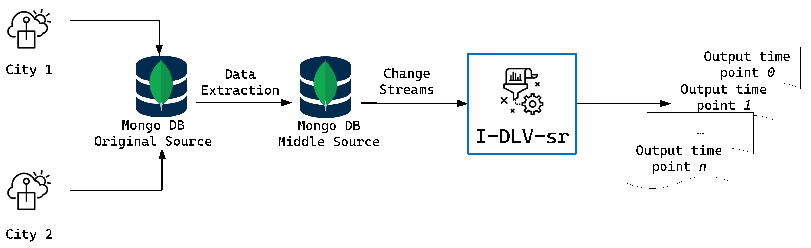
4.1. Experimental Setting

The experiments have been performed on a DELL XPS machine equipped with a 2.2 GHz Intel® Xeon® E5-2650 CPU, with 12 cores and 64GB of RAM. The tested query modellings are those described in Section 3. All modellings along with instructions for properly reproducing experiments are reported at the dedicated GitHub repository https://github.com/DeMaCS-UNICAL/EnviroStream (accessed on 1 May 2023). As a performance measure, we took into account the processing-time latency (latency for short): for each time point, we measured the delay between the time at which the input relative to such time point is received and the time at which the system produces the corresponding output. In other words, latency measures the period of time the system takes to reason on a given input.
To fairly test all queries in the same setting, we emulated a real environment in which I-DLV-sr consumes the dataset at hand from a MongoDB source. Intuitively, testing all queries over data extracted in different time periods could result in an unfair comparison, since environmental and climate data vary over time. Therefore, we cannot use the original MongoDB source, which continuously receives new data.
To show I-DLV-sr reactivity in practice, we simulated real-time data arrival via the MongoDB “Change Streams” functionality, allowing a client to subscribe to all data changes on a database and immediately react to them. Figure 2 exemplifies the adopted pipeline. In more detail, to run each query, we populated an initially empty MongoDB database (MongoDB Middle Source in Figure 2) according to the dataset at hand, and I-DLV-sr continuously retrieved data from this database. Specifically, data are ingested into the MongoDB database in real-time, at the same frequency they arrived to the original source, i.e., approximately every 2 min, as specified in Section 2.
In this setting, in order to run the queries allowing I-DLV-sr to read new data from a MongoDB source and obtain the expected output, users should execute the following command:
  • java –jar I–DLV–sr.jar \
  •   ––program=path/to/query/encoding \
  •   ––py–script=path/to/external.py \
  •   ––mongodb \
  •   ––mongodb–config=path/to/mongodb/config.yaml \
  •   ––t–unit=min ––windows–unit=min ––now–format=min,
where the option --program is used to specify the query encoding; --py-script is used to provide a path to a script containing Python functions which define the behaviour of external atoms (if any); --mongodb and --mongodb-config are used to enable I-DLV-sr to read data stream from a MongoDB source as specified in the given configuration file in the YAML format; the remaining options are used to set the reasoning time unit in minutes.
In more detail, in order to run, e.g., query 4 over I-DLV-sr, the following parameters must be specified:
  • java –jar I–DLV–sr.jar \
  •   ––program=EnviroStream/queries/program/q4.idlvsr \
  •   ––py-script=EnviroStream/queries/script/external.py \
  •   ––mongodb \
  •   ––mongodb–config=EnviroStream/queries/config/q4.yaml \
  •   ––t–unit=min ––windows-unit=min ––now–format=min.
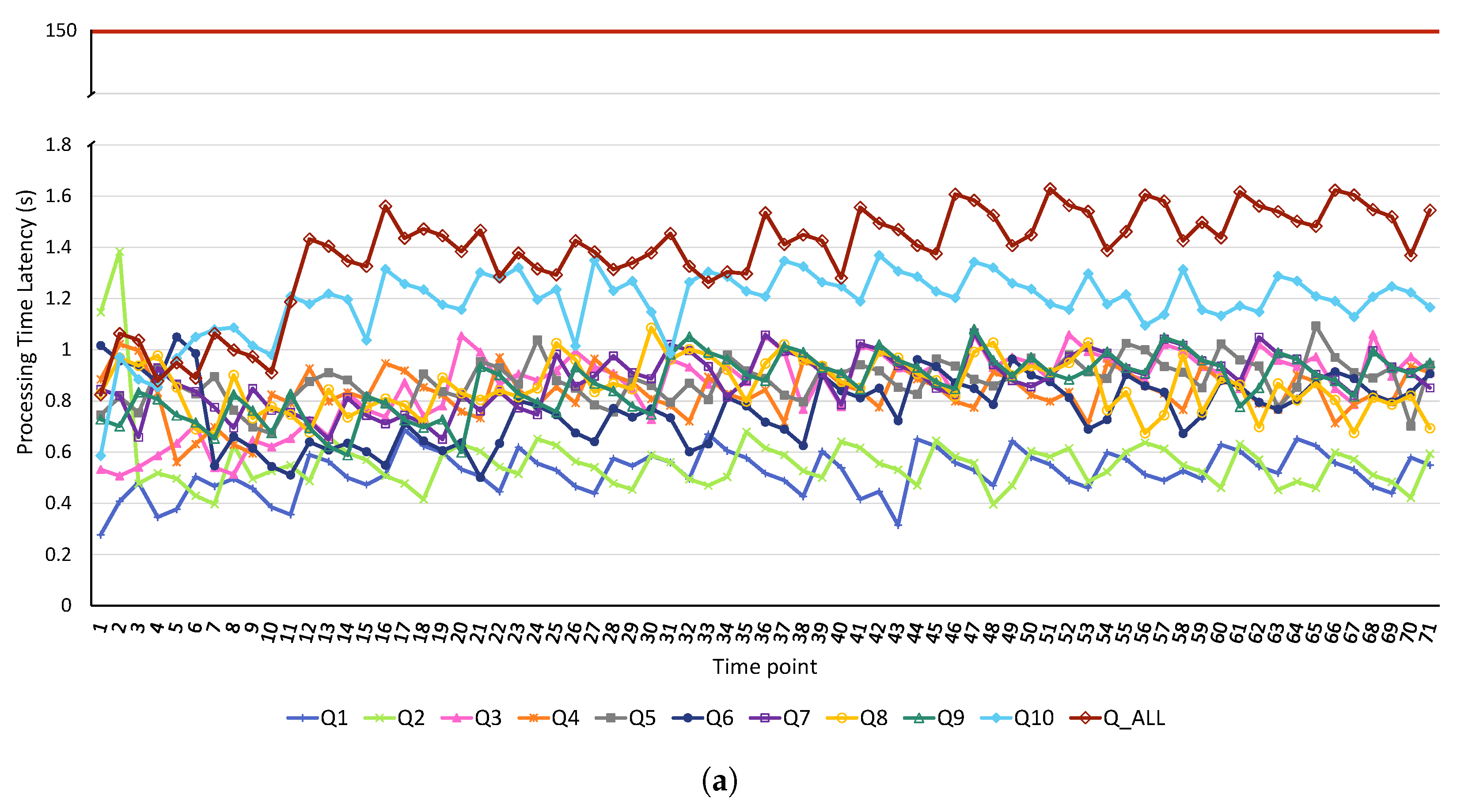
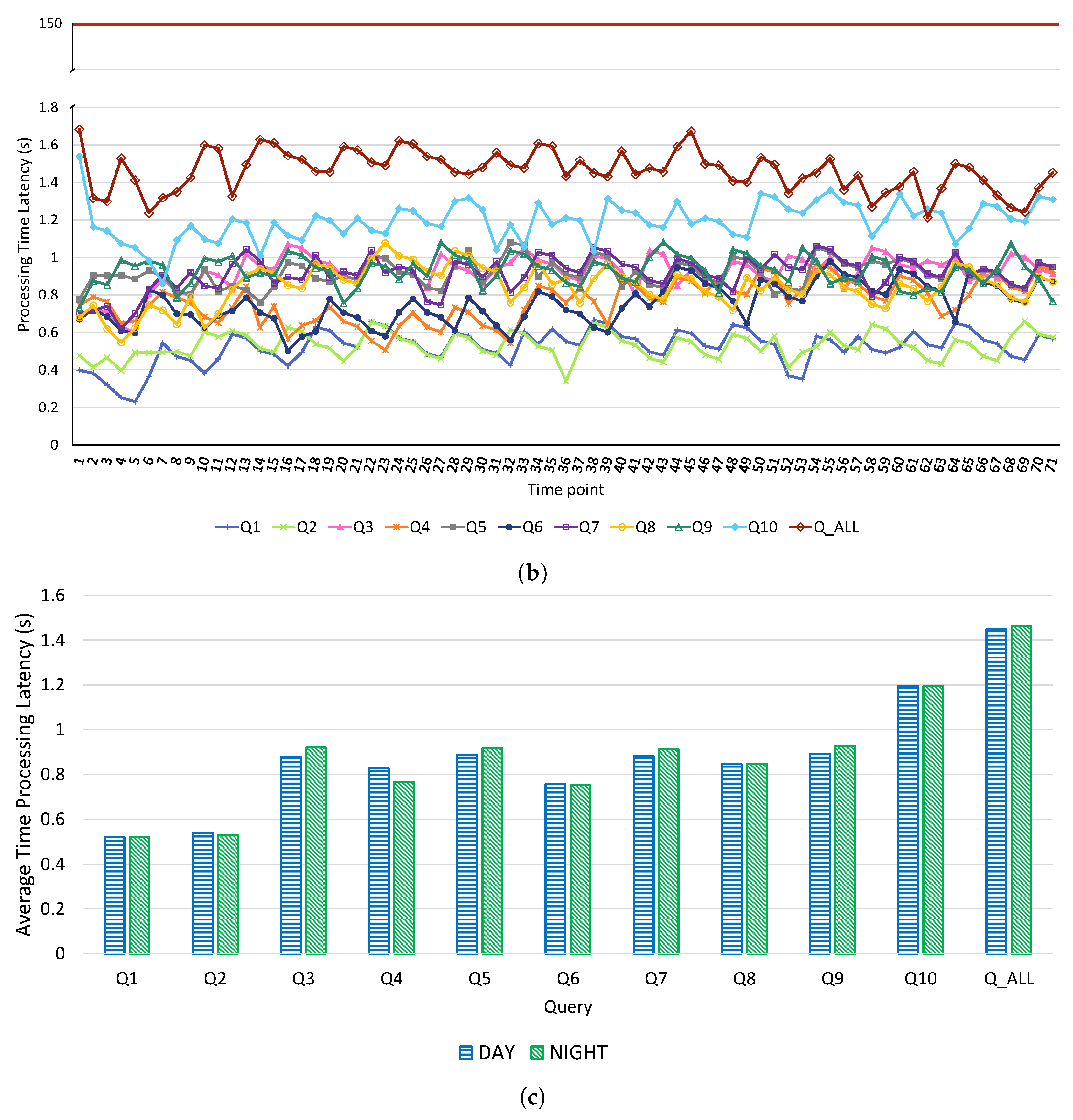
Note that, in this setting, the time required to execute a single query is at least equal to the time interval represented by the dataset, i.e., given a dataset of three hours (like day or night), the execution of each query takes at least 3 h. We remark that, in order to simulate the arrival of data to the MongoDB source across the whole observed period of 3 months, the execution of each query would require at least 3 months. Indeed, Stream Reasoning systems are conceived to process data in real-time, and in case the time spent to reason on a bunch of data is less than the arrival time of the next bunch, systems have to wait because there are no new inputs to reason on. For this reason, testing all the 11 queries (including Q _ A L L ), in a fair sequential mode, on the whole 3 months data would require about 33 months, which would be unfeasible. Moreover, to evaluate the real-time reasoning capabilities of I-DLV-sr in practice, we implemented a web application as discussed in Section 5.

4.2. Results

Figure 3 reports the latency. In further detail, Figure 3a,b show how the latency (y-axis) varies over the time points (x-axis) per each query over the day and the night, respectively; the red line indicates the average time between the arrival of a bunch of data and the next one. Furthermore, Figure 3c reports the average latency computed over all time points on both datasets. Note that a time point corresponds to a measuring time, i.e., a timestamp at which a bunch of data has been produced by a station.
The results show that the latency is far below the red line in all time points for each query, including Q _ A L L , which is, as expected, the one requiring more computational effort. On average, performance over day and night datasets are quite similar, as evidenced in Figure 3c. Taking a closer look, we observe that in Q 1 and Q 2 the latency is always less than 0.7 s since they require to reason over smaller windows w.r.t. the other queries. Slightly higher latency times are registered for Q 3 , Q 4 , Q 5 , Q 6 , Q 7 , Q 8 , and Q 9 whose trends vary between 0.5 and 1.1 s; indeed, these queries have been designed to be computationally more expensive and to involve larger windows. The highest latency times are obtained on Q 10 and Q _ A L L : the former ranges between 0.8 and 1.5 s, whereas the latter between 1.1 and 1.7 s. The reason behind this behaviour is the modelling of Q 10 , in which streaming literals are recursively evaluated over past time points. In turn, the trend of Q _ A L L , which consists of the union of all queries, is influenced by Q 10 . Finally, it is worth noting that the performance on Q _ A L L is not given by the sum of latencies over the 10 queries because several queries share portions of programs, as reported in Section 3.

5. Online Reasoning over EnviroStream via the I-DLV-sr System

In order to practically assess online reasoning of I-DLV-sr on the herein presented EnviroStream benchmark, we deployed a web application available at https://experiments.demacs.unical.it/ (accessed on 1 May 2023). The web app features some plots showing aggregated information, used within the queries of EnviroStream, over real-time data collected by the weather stations of both cities, namely:
  • average PM 10 emissions in the last 10 min;
  • average PM 2.5 emissions in the last 10 min;
  • number of noise measures above the recommended WHO thresholds (i.e., 65 during day and 55 during night);
  • current Humidex level;
  • total millimeters of rain fallen in the last hour;
  • current Beaufort level on the basis of the average wind speed in the last 10 min.
The plots are generated on the basis of data produced by I-DLV-sr, which runs in the back-end, continuously receiving new data from the MongoDB source storing measures from both weather stations. Note that, differently from the experimental setting of Section 4, in the web app, I-DLV-sr directly retrieves data from the real MongoDB source communicating with the stations.

6. Conclusions

EnviroStream is a benchmark for evaluating Stream Reasoning systems in real dynamic settings over weather and environmental data; it currently provides data from weather stations in two European cities, but we plan to extend the deployment of base stations to other cities in the near future. To date, it consists of 10 queries for monitoring some crucial ambient topics: air quality, noise pollution, heatwave, rain intensity, and wind force. The queries have been conceived by studying the recommendations of major organizations promoting human health and monitoring climate change, and they have been designed in such a way as to cope with the most commonly needed expressive capabilities in Stream Reasoning systems. As a baseline, we also discussed in detail how I-DLV-sr, a recent Stream Reasoning system, can be adopted to model the queries and reason over EnviroStream datasets, and we outlined with a proof-of-concept example how queries in EnviroStream can be expressed in a different language. Moreover, we released a publicly accessible web site showcasing the online real-time reasoning performed by I-DLV-sr in the featured scenario.
As pointed out in Section 1, this work aimed at overcoming the current difficulties in evaluating Stream Reasoning systems, with a special focus on logic-based ones. The present work contributes to increasing the availability of Stream Reasoning benchmarks for both the logic-programming and the RSP settings; its applicability to different kinds of systems is granted by the wide range of available data formats. Furthermore, data are continuously injected in real-time from the available sensors, thus producing over time an incrementally growing amount of data that are periodically released. To the best of our knowledge, this is a unique feature of the herein presented benchmark.
In conclusion, this work provides a foundation for future studies, offering a baseline for comparing Stream Reasoning systems functionalities, capabilities and performance. Concerning functionalities, EnviroStream is challenging as it requires to deal with real-time data stream processing and incompleteness, caused, e.g., when stations delay data transmission because of network issues. Moreover, the queries pose a modeling challenge for comparing the expressive capabilities of the system at hand. Eventually, EnviroStream can be adopted to test performance as systems are required to reason over data coming at a non-fixed rate without losing responsiveness. We believe that it is particularly interesting to evaluate systems on large-scale datasets. We thus provided the large dataset featuring all data we gathered since the stations became operational, i.e., about three months. For the same reason, we developed the aforementioned web application, proving the I-DLV-sr resilience over real-time and long-term reasoning.
We plan to enrich EnviroStream in both datasets and queries through the installation of further stations so that for each city, we can combine data coming from more than one station and begin to consider some form of weather forecasting. This way, it will be possible to have a more comprehensive and accurate view of the weather conditions in each city.

Author Contributions

Conceptualization, F.P. and J.Z.; methodology, F.P. and J.Z.; software, E.M., F.P and J.Z.; validation, E.M., F.P. and J.Z.; formal analysis, F.P. and J.Z.; investigation, F.P. and J.Z.; resources, F.C., S.P. and G.T.; data curation, E.M., F.P. and J.Z.; writing—original draft preparation, F.P. and J.Z.; writing—review and editing, F.C., E.M., F.P., S.P., G.T. and J.Z.; visualization, F.P. and J.Z.; supervision, F.C., F.P., S.P., G.T. and J.Z.; project administration, F.C., S.P. and G.T.; funding acquisition, F.C., S.P. and G.T. All authors have read and agreed to the published version of the manuscript.

Funding

This work has been supported by the PNRR project FAIR—Future AI Research (PE00000013), Spoke 9—Green-aware AI, under the NRRP MUR program funded by the “NextGenerationEU”, and by the project PRIN PE6, Title: “Declarative Reasoning over Streams”, funded by the Italian Ministero dell’Università, dell’Istruzione e della Ricerca (MIUR), CUP:H24I17000080001, and by the project “Smart Cities Lab” (CUP J89J21009750007) funded on POR FESR-FSE Calabria 2014–2020.

Data Availability Statement

We provide three datasets of different sizes in CSV and JSON format, freely available at https://doi.org/10.5281/zenodo.8142369 (accessed on 1 May 2023): day, night and large. day is a three hour dataset on a Wednesday afternoon (15 March 2023 from 12:00 p.m. to 03:00 p.m.), night is a three hour dataset on a Saturday night (from 11 March 2023 10:00 p.m. to 12 March 2023 01:00 a.m.) and large is a bigger dataset featuring detections from 1 January 2023 12:00 a.m. to 28 March 2023 11:59 p.m. All dataset concern weather and environmental data of two European cities, whose names are omitted for anonymity reasons. Data are collected through weather stations scattered in each city.

Acknowledgments

The authors would like to thank the DLVSystem Srl Company (https://www.dlvsystem.com (accessed on 1 May 2023)) for providing access to valuable data and the fruitful collaboration; furthermore, they want to thank Giovanni Laboccetta for the fruitful discussions about the application domains.

Conflicts of Interest

The authors declare no conflict of interest.

Abbreviations

The following abbreviations are used in this manuscript:
ASPAnswer Set Programming
SRStream Reasoning
SPStream Processing
CEPComplex Event Processing
KRRKnowledge Representation and Reasoning
PMParticulate Matter

References

  1. Dell’Aglio, D.; Valle, E.D.; van Harmelen, F.; Bernstein, A. Stream reasoning: A survey and outlook. Data Sci. 2017, 1, 59–83. [Google Scholar] [CrossRef] [Green Version]
  2. Mileo, A.; Dao-Tran, M.; Eiter, T.; Fink, M. Stream Reasoning. In Encyclopedia of Database Systems, 2nd ed.; Springer: Berlin/Heidelberg, Germany, 2018. [Google Scholar]
  3. Barbieri, D.F.; Braga, D.; Ceri, S.; Valle, E.D.; Grossniklaus, M. C-SPARQL: A Continuous Query Language for RDF Data Streams. Int. J. Semantic Comput. 2010, 4, 3–25. [Google Scholar] [CrossRef] [Green Version]
  4. Phuoc, D.L.; Dao-Tran, M.; Parreira, J.X.; Hauswirth, M. A Native and Adaptive Approach for Unified Processing of Linked Streams and Linked Data. In International Semantic Web Conference; Lecture Notes in Computer Science; Springer: Berlin/Heidelberg, Germany, 2011; Volume 7031, pp. 370–388. [Google Scholar]
  5. Hoeksema, J.; Kotoulas, S. High-Performance Distributed Stream Reasoning Using s4. In Ordring Workshop at ISWC; 2011; Available online: http://iswc2011.semanticweb.org/fileadmin/iswc/Papers/Workshops/OrdRing/paper_8.pdf (accessed on 1 May 2023).
  6. Pham, T.; Ali, M.I.; Mileo, A. C-ASP: Continuous ASP-Based Reasoning over RDF Streams. In Logic Programming and Nonmonotonic Reasoning; Lecture Notes in Computer Science; Springer: Berlin/Heidelberg, Germany, 2019; Volume 11481, pp. 45–50. [Google Scholar]
  7. Schneider, P.; Alvarez-Coello, D.; Le-Tuan, A.; Duc, M.N.; Phuoc, D.L. Stream Reasoning Playground. In Proceedings of the 19th European Semantic Web Conference, Hersonissos, Greece, 29 May–2 June 2022; Lecture Notes in Computer Science. Springer: Berlin/Heidelberg, Germany, 2022; Volume 13261, pp. 406–424. [Google Scholar]
  8. Phuoc, D.L.; Dao-Tran, M.; Pham, M.; Boncz, P.A.; Eiter, T.; Fink, M. Linked Stream Data Processing Engines: Facts and Figures. In Proceedings of the 11th International Semantic Web Conference, Hangzhou, China, 23–27 October 2022; Lecture Notes in Computer Science. Springer: Berlin/Heidelberg, Germany, 2012; Volume 7650, pp. 300–312. [Google Scholar]
  9. Nguyen, T.N.; Siberski, W. SLUBM: An Extended LUBM Benchmark for Stream Reasoning. In Proceedings of the 2nd International Workshop on Ordering and Reasoning, OrdRing 2013, Co-located with the 12th International Semantic Web Conference (ISWC 2013), Sydney, Australia, 22 October 2013; Volume 1059, pp. 43–54. [Google Scholar]
  10. Ali, M.I.; Gao, F.; Mileo, A. CityBench: A Configurable Benchmark to Evaluate RSP Engines Using Smart City Datasets. In International Semantic Web Conference; Lecture Notes in Computer Science; Springer: Berlin/Heidelberg, Germany, 2015; Volume 9367, pp. 374–389. [Google Scholar]
  11. Tommasini, R.; Balduini, M.; Valle, E.D. Towards a Benchmark for Expressive Stream Reasoning. In Proceedings of the 2nd RDF Stream Processing (RSP 2017) and the Querying the Web of Data (QuWeDa 2017) Workshops Co-Located with 14th ESWC 2017 (ESWC 2017), Portoroz, Slovenia, 28–29 May 2017; Volume 1870, pp. 26–36. [Google Scholar]
  12. Pitsikalis, M.; Artikis, A.; Dreo, R.; Ray, C.; Camossi, E.; Jousselme, A. Composite Event Recognition for Maritime Monitoring. In Proceedings of the 13th ACM International Conference on Distributed and Event-Based Systems, Darmstadt, Germany, 24–28 June 2019; ACM: Boston, MA, USA, 2019; pp. 163–174. [Google Scholar]
  13. Calimeri, F.; Manna, M.; Mastria, E.; Morelli, M.C.; Perri, S.; Zangari, J. I-DLV-sr: A Stream Reasoning System based on I-DLV. Theory Pract. Log. Program. 2021, 21, 610–628. [Google Scholar] [CrossRef]
  14. Huler, S. Defining the Wind: The Beaufort Scale and How a 19th-Century Admiral Turned Science into Poetry; Crown: New York, NY, USA, 2007. [Google Scholar]
  15. Gelfond, M.; Lifschitz, V. Classical Negation in Logic Programs and Disjunctive Databases. New Gener. Comput. 1991, 9, 365–386. [Google Scholar] [CrossRef] [Green Version]
  16. Brewka, G.; Eiter, T.; Truszczynski, M. Answer set programming at a glance. Commun. ACM 2011, 54, 92–103. [Google Scholar] [CrossRef]
  17. Lifschitz, V. Answer Set Programming; Springer: Berlin/Heidelberg, Germany, 2019. [Google Scholar]
  18. Calimeri, F.; Ianni, G.; Pacenza, F.; Perri, S.; Zangari, J. ASP-based Multi-shot Reasoning via DLV2 with Incremental Grounding. In Proceedings of the 24th International Symposium on Principles and Practice of Declarative Programming, Tbilisi, Georgia, 20–22 September 2022; ACM: Boston, MA, USA, 2022; pp. 2:1–2:9. [Google Scholar]
  19. Ianni, G.; Pacenza, F.; Zangari, J. Incremental maintenance of overgrounded logic programs with tailored simplifications. Theory Pract. Log. Program. 2020, 20, 719–734. [Google Scholar] [CrossRef]
  20. Beck, H.; Eiter, T.; Folie, C. Ticker: A system for incremental ASP-based stream reasoning. Theory Pract. Log. Program. 2017, 17, 744–763. [Google Scholar] [CrossRef] [Green Version]
  21. Eiter, T.; Ogris, P.; Schekotihin, K. A Distributed Approach to LARS Stream Reasoning (System paper). Theory Pract. Log. Program. 2019, 19, 974–989. [Google Scholar] [CrossRef] [Green Version]
  22. Beck, H.; Dao-Tran, M.; Eiter, T. LARS: A Logic-based framework for Analytic Reasoning over Streams. Artif. Intell. 2018, 261, 16–70. [Google Scholar] [CrossRef]
Figure 1. Σ 1 : an example of a (partial) stream.
Bdcc 07 00135 g001
Figure 2. Experimental set-up.
Bdcc 07 00135 g002
Figure 3. Performance of I-DLV-sr over the day dataset (a), the night dataset (b), and average latency per time point over both datasets (c).
Bdcc 07 00135 g003aBdcc 07 00135 g003b
Table 1. Examples of entailment of ground streaming literals.
Positive LiteralHoldsNegative LiteralHolds
b(5) always in [2 sec]Nonot b(5) always in [2 sec]Yes
a(3) always in [2 sec]Yesnot a(3) always in [2 sec]No
a(3) always in {0,2,3}Nonot a(3) always in {0,2,3}Yes
b(5) count 2 in [2 sec]Nonot b(5) count 2 in [2 sec]Yes
b(5) count 1 in [2 sec]Yesnot b(5) count 1 in [2 sec]No
b(5) count 1 in {1,3}Nonot b(5) count 1 in {1,3}Yes
b(5) at least 2 in [2 sec]Nonot b(5) at least 2 in [2 sec]Yes
b(5) at least 1 in [2 sec]Yesnot b(5) at least 1 in [2 sec]No
b(5) at least 2 in {1,3}Yesnot b(5) at least 1 in {1,3}No
a(3) at most 2 in [2 sec]Nonot a(3) at most 2 in [2 sec]Yes
b(5) at most 1 in [2 sec]Yesnot b(5) at most 1 in [2 sec]No
b(5) at most 1 in {0,2}Yesnot b(5) at most 1 in {0,2}No
Table 2. Input atoms.
TypeAtomMeaning
Staticstation(C)Weather station of city C
maximum_allowed_pm10(X)X is the maximum PM 10 allowed
maximum_allowed_pm2_5(X)X is the maximum PM 2.5 allowed
day_threshold(X)X is the noise limit during day
night_threshold(X)X is the noise limit during night
threshold_1_hour(X)X is the noise exposure limit over a hour
light_rain_threshold(X)X is the light rain threshold over a hour
heavy_rain_threshold(X)X is the heavy rain threshold over a hour
Dynamicpm10(C,V)V is the current PM 10 level in city C
pm2_5(C,V)V is the current PM 2.5 level in city C
noise(C,V)V is the current noise in city C
temperature(C,V)V is the current temperature in city C
humidity(C,V)V is the current humidity in city C
rain(C,V)V is the current rain in city C
wind_speed(C,V)V is the current wind speed in city C
Disclaimer/Publisher’s Note: The statements, opinions and data contained in all publications are solely those of the individual author(s) and contributor(s) and not of MDPI and/or the editor(s). MDPI and/or the editor(s) disclaim responsibility for any injury to people or property resulting from any ideas, methods, instructions or products referred to in the content.

