Comparative Study of Parameter Identification with Frequency and Time Domain Fitting Using a Physics-Based Battery Model

Abstract

Parameter identification with the pseudo-two-dimensional (p2D) model has been an important research topic in battery engineering because some of the physicochemical parameters used in the model can be measured, while some can only be estimated or calculated based on the measurement data. Various methods, either in the time domain or frequency domain, have been proposed to identify the parameters of the p2D model. While the methods in each domain bring their advantages and disadvantages, a comprehensive comparison regarding parameter identifiability and accuracy is still missing. In this present work, some selected physicochemical parameters of the p2D model are identified in four different cases and with different methods, either only in the time domain or with a combined model. Which parameters are identified in the frequency domain is decided by a comprehensive analysis of the analytical expression for the DRT spectrum. Finally, the parameter identifiability results are analyzed and the validation results with two highly dynamic load profiles are shown and compared. The results indicate that the model with ohmic resistance and the combined method achieves the best performance and the average voltage error is at the level of 12 mV.

1. Introduction

To build a more robust power grid with growing renewable energy sources and to enable an electrified transportation system, lithium-ion batteries (LIBs) are being increasingly deployed in various sectors, such as stationary energy storage systems and electrical vehicles. While the demand for LIBs is increasing, a longer lifespan and safer operation should still be guaranteed. To realize a better design of BMS and ensure a safer operation, an accurate identification of the cell parameters is imperative [1]. In most cases, to estimate the cell parameters, a proper objective function will be chosen and an optimization problem will be established to identify the parameters of interest [2]. Generally, according to the input data for the optimization problem, the identification methods can be roughly classified into two groups: time domain and frequency domain methods [3]. Time domain methods use the measurement data gathered in the time domain, such as charging/discharging curves or pulse test data; frequency domain methods usually refer to electrochemical impedance spectroscopy (EIS), where the cell impedance is measured as a function of the frequency of the excitation signal. Due to the different measurement principles, parameters are identified with different identifiabilities and accuracies [3,4].

1.1. Parameter Identification in Time Domain

For the time domain methods, first, a preselected model is built to model the internal physicochemical processes of the LIBs. Depending on the desired model complexity and comprehensiveness, the equivalent circuit model (ECM), reduced-order model (ROM) based on the physicochemical model, and full-order physicochemical model (PCM) are available as potential candidates. The ECM is able to model certain physicochemical processes using specific circuit elements such as resistance, capacitance, and inductance. On the one hand, the ECM models the LIBs only in a simplified way, many complicated electrochemical processes are modeled with a lumped circuit element or even simply neglected; therefore, some physicochemical parameters are not given in the ECM. On the other hand, due to its easy implementation and fast computational speed, the ECM is favored in real-time or on-board applications [5,6,7]. The PCM describes the physicochemical processes with the first principle equations and the model output (voltage, current, temperature, etc.) is directly related to the fundamental physicochemical parameters [8,9,10,11,12,13]. The PCM usually consists of a group of coupled partial differential equations (PDEs) and the required computational effort is much higher than that of the ECM. Normally, the PCM must be solved using numerical methods such as the finite-element-method, which prevents it from real-time applications and large-scale simulation studies. To resolve the computational burden issue and meanwhile keep the accuracy loss on an acceptable level, the ROM has been developed by neglecting the less important processes or conducting mathematical simplification [14,15,16,17,18,19,20,21,22]. Compared to the full-order PCM, the computational demand of the ROM can be largely reduced and the accuracy loss can be generally kept to an acceptable level.

As the next step for parameter identification, an objective function must be selected and an optimization program with an appropriate algorithm is established to solve the parameter identification program. Due to the strongly nonlinear nature of the LIB models, the resulting optimization problem is strongly nonlinear as well and a carefully chosen algorithm must be applied to solve the problem. Various nonlinear optimization algorithms have been applied to the parameter identification problem of LIBs, including gradient-based or Hessian-based methods [6,15,16], heuristic methods [5,9,12,17], and statistical methods [10,13]. ECM-based parameter identification has a low demand for computational capacity, while a direct connection with the fundamental physicochemical parameters is usually unclear or even missing, which is a considerable drawback for the identification of physicochemical parameters and cell design. The PCM is the most comprehensive model, and relates the physicochemical and geometric parameters directly to the model output.

While most parameter identification studies focus on model development and optimization algorithms, only a small part of the works considers the parameter identifiability and sensitivity issues. Forman et al. conducted a parameter identification test and identifiability analysis using the Fisher information [12], where the local parameter identifiability and variance were determined. Berliner et al. applied the Markov chain Monte Carlo (MCMC) method to explore the parameter space and identified the quantitative nonlinear correlation among three parameters [13]. The characterization of the quantitative correlation (especially nonlinear) among multiple (more than two) parameters is an essential step, because the emphasis has been mostly laid on the analysis of parameter sensitivity and correlation between only two parameters and an important fact has been neglected: a coordinated change of multiple parameters (more than two) may lead to the same model output and a unique global optimum may not exist. As a result, the parameter identifiability analysis suggests that simply minimizing the objective function and analyzing the local parameter sensitivity cannot guarantee a reliable and physically meaningful identification result.

1.2. Parameter Identification in Frequency Domain

Parameter identification in the frequency domain is conducted in a similar manner, where the desired impedance model is selected and an optimization program is established to estimate the model parameters. Various models have been used to identify the cell parameters, including the ECM [23,24,25,26,27,28], ROM [29,30,31], and PCM [32,33,34,35]. The identification methods used in the aforementioned literature are all based on nonlinear optimization methods and naturally are faced with the same issues as in the time domain method. For example, the same impedance data can be fitted using different equivalent circuits with different structures and numbers of circuit elements [36], thus the results could be quite confusing. Moreover, many local optima may exist and it needs more effort to find the global optimum. Recently, many researchers proposed to use the method distribution of relaxation times (DRT) to evaluate the impedance data, which is based on linear optimization and the identifiability issue is no more considerable [37,38,39,40,41,42]. However, an appropriate model is still necessary for the interpretation of the DRT results. Until now, most models that have been used to interpret the DRT results are based on the ECM and a direct relation to the physicochemical parameters is still missing [42,43,44,45,46,47].

1.3. Comparison and Unification of Time Domain and Frequency Domain Parameter Identification Methods

Both time domain methods and frequency domain methods characterize the cell parameters using a selected model. Due to the different properties of both methods, different parameters may be estimated with different identifiabilities. Laue et al. [4] investigated the sensitivity of the p2D model by considering the data both in the time domain and frequency domain. However, no universal analysis was made regarding the identifiability of the parameters with impedance data and the results were not validated. Wimarshana et al. [3] investigated the parameter sensitivity by considering the measurement data in both the time and frequency domains. Again the parameters were not identified and the results were not validated and compared, which means that the effectiveness of the combined procedures is still unknown. After the parameters have been identified, the estimation results are usually simply validated by inserting the estimated parameters back into the model and the model will be simulated in a few limited application scenarios, mostly only with constant charging/discharging current. In most cases, the parametrized model gives a moderate to low error. As a result, three important questions are raised regarding the issues mentioned above: (1) How reliable are the parameters identified using the time domain fitting? (2) If a combined method with both time and frequency domain data is applied, which parameters will be better identified with impedance data and why? (3) Does a combined identification method with both the time domain and frequency domain data optimize the parameter identifiability and lead to better accuracy for the validation? In the present work, we will focus on the three questions raised above and try to find the answers.

The rest of the work is organized as follows: in Section 2, the used models and parameter identification procedures will be introduced; in Section 3, lab experiments are conducted to identify the model parameters and investigate the identifiability with each method; in Section 4, the results will be discussed; Section 5 concludes the work.

2. Theory and Model Development

In this section, the theoretical fundamentals, procedures, and algorithms used for different parameter identification methods will be introduced. Then the methodology for the parameter identifiability and correlation analysis will be explained.

2.1. Parameter Identification in the Time Domain

Since being proposed by Doyle and Newman [48,49,50], the p2D model has been widely applied to the design, simulation, and parameter identification of LIBs. The p2D model describes the internal physicochemical processes using a group of coupled PDEs, thus requiring a high computation capability. Therefore, a direct application of the p2D model to parameter identification is rather time-consuming and inefficient because the model must be iteratively computed a large number of times depending on the parameter identifiability and convergence rate. As an alternative, the reduced-order model (ROM) has been proposed by researchers to improve the computation speed, while the accuracy loss is nearly negligible when the model order is properly chosen. In one of our previous works, a ROM using the Chebyshev orthogonal collocation method has been developed and validated [20]. According to the conducted simulation experiment, it is found that the model with an (8, 5, 7) collocation point configuration in the anode, separator, and cathode, respectively, can well approximate the relevant transport processes and the computation demand is much lower with a degree of freedom (DOF) of ca. 160. The simulation time of one charging/discharging process $t_{\mathrm{CH}/\mathrm{DCH}}$ with Matlab/Simulink is about 0.2 s, the model setting is summarized in

Table 1. Summary of the model setting for ROM used for parameter identification test.

Model Type	Polynomial Type	(nn, ns, np)	DOF	tCH/DCH
ROM with p2D	Chebyshev	($8,5,7$)	ca. 160	0.2 s

.

To assess the quality of the parameter estimation results, various methods have been proposed to quantify the identifiability of the estimated parameters. Commonly used methods include the once-at-a-time (OAT) method [3,51], Fisher information matrix (FIM) [12] and Sobol’ indices [4,52]. In this present work, we choose to use Bayesian statistics combined with the MCMC sampling algorithm for the parameter estimation and identifiability characterization. The reasons for using the Bayesian MCMC method are as follows: (1) It quantifies the global identifiability of the parameters because the parameter values are randomly sampled in the whole defined parameter space. If the sample size is big enough, an empirical distribution close to the real posterior distribution can be obtained. (2) The posterior distribution of the parameters is able to characterize the unidentifiability when it arises either from non-sensitivity or parameter correlation, in both cases, a posterior distribution with a wide credible interval can be observed. (3) The credible interval and thus the identifiability of parameters can easily be visualized and computed with the resulting parameter distribution.

In practical applications, the measurement data is generally exposed to a normally distributed noise with a zero mean:

$$V_{\mathrm{m}}={\widehat{V}}_{\mathrm{m}}+{ϵ}_{\mathrm{e}}$$

(1)

where $V_{\mathrm{m}}$ is the measured cell voltage, ${\widehat{V}}_{\mathrm{m}}$ is the cell voltage without noise, ${ϵ}_{\mathrm{e}}$ is the measurement noise, and the following distribution is assumed:

$${ϵ}_{\mathrm{e}}\sim \mathcal{N}(0,{\sigma }_{\mathrm{e}}^2)$$

(2)

where ${\sigma }_{\mathrm{e}}$ is the standard deviation of the noise and is set to 10 mV in this work. As usually there is no information about the variance of the voltage noise, other proper values can be used as well and the results should not vary because this is equivalent to adding a constant to the logarithmic object function values. By using Bayes’ theorem, the conditional probability of the model parameter $\theta$, given the measurement data, is defined as:

$$P\left(\theta \right|V_{\mathrm{m}})=\frac{P\left(V_{\mathrm{m}}\right|\theta )P\left(\theta \right)}{P\left(V_{\mathrm{m}}\right)}$$

(3)

where $P\left(\theta \right)$ is the prior distribution for the parameters, which is based on the prior knowledge of the parameter. In certain situations, enough information can be collected to define an informative prior distribution for the parameter, for example the beta distribution. In this present work, the prior distribution $P\left(\theta \right)$ is assumed to be uniformly distributed between its upper and lower bound because there is no information available to define an informative prior distribution. In our application, the measurement data $V_{\mathrm{m}}$ are given with a certain constant distribution, thus $P\left(V_{\mathrm{m}}\right)$ can be assumed to be a constant. As a result, the conditional probability can be reformulated as:

$$P\left(\theta \right|V_{\mathrm{m}})\propto P\left(V_{\mathrm{m}}\right|\theta )$$

(4)

The probability of observing the measurement data $V_{\mathrm{m}}$ is equivalent to that of observing the measurement noise ${ϵ}_{\mathrm{e}}$ given the model parameter $\theta$ and can be defined as follows:

$$P\left(V_{\mathrm{m}}\right|\theta )=\prod _{i=1}^{N_{\mathrm{m}}}\frac{1}{{\sigma }_{\mathrm{e}}\sqrt{2\pi }}\exp \left(-\frac{1}{2}{\left(\frac{V_{\mathrm{m},i}-{\widehat{V}}_{\mathrm{m},i}\left(\theta \right)}{{\sigma }_{\mathrm{e}}}\right)}^2\right)$$

(5)

where i represents the index of the measurement data points and $N_{\mathrm{m}}$ is the total number of the measured voltage data points. To sample the parameter space, the adaptive Metropolis–Hastings MCMC algorithm is used to generate the parameter samples [53], the sample size for each test is set to 50,000 and the desired acceptance rate is set to 0.23 [54].

While the OAT metrics only characterize the sensitivity and possible correlation of a parameter at a specific location, the Bayesian MCMC sampling results can well characterize both properties globally. Therefore, to quantify the general identifiability of a parameter, the following sensitivity index (SI) $\mathcal{S}$ is defined:

$$\mathcal{S}=\frac{{\theta }_{\max }-{\theta }_{\min }}{\mathcal{L}}$$

(6)

where ${\theta }_{\max }$ and ${\theta }_{\min }$ are the upper and lower bound of the parameter, respectively, and $\mathcal{L}$ is the width of the $95\%$ credible interval (CI) of the parameter. Unlike the equal-tailed-interval (ETI), in this work the CI of each parameter is calculated using the highest-density-probability (HDP) concept, where the interval with the highest probability density is chosen to calculate the CI, as some parameters, such as the diffusion coefficients, can range for multiple orders of magnitude, the logarithmic scale is used to calculate the SI. A high sensitivity index implies that the parameter is confined in a small credible interval compared to the bounds and thus can be reliably estimated, whereas a low SI indicates that the parameter is practically unidentifiable.

2.2. Parameter Identification in Frequency Domain

According to our previous works on the interpretation of a DRT spectrum using a physics-based impedance model, the diffusion coefficient in the solid and liquid phases and the interface parameters such as the kinetic reaction rate constant and the film resistance can be directly determined, if the related geometric parameters are known. For the Bruggeman coefficients and the conductivities in the solid and liquid phases, the corresponding contribution only appears in the ohmic resistance of the cell and possibly also in the high-frequency dispersion part of the impedance/DRT. The Bruggeman coefficients also contribute to the effective transportation in the liquid phase. However, the bulk value of the liquid diffusivity is usually unknown, thus it is still impossible to estimate the Bruggeman coefficients using the liquid phase diffusion. Considering that the dispersion of the DRT spectra in the high-frequency area is usually blurred by contributions of other processes in practical applications and it is impossible to separate the impedance contribution from the anode, separator, and cathode, the conductivity in the solid/liquid phase and the Bruggeman coefficient can be considered as unidentifiable with the DRT method.

Rabissi et al. [55] investigated the sensitivity and identifiability of the physicochemical parameters with a physicochemical impedance model. However, no general conclusions have been made with the impedance model regarding the parameter identifiability. To have a quantitative conclusion on the identifiability, a numerical analysis is still necessary. Based on the analysis made in our previous works, where the analytical expressions for the DRT have been derived and interpreted, a universal conclusion can be made regarding the identifiability of the physicochemical parameters used in the p2D model. Due to the fact that the DRT spectrum ($\tau$ domain) is actually equivalent to the raw impedance data (f domain), the conclusions made with the DRT spectrum are also valid for the impedance. In the DRT spectrum, a process is characterized mainly by two key features: (1) the time constant of the peak (or the dominant peak) representing the process; (2) the area under the peak (or the dominant peak) which represents the polarization resistance of the process. As a result, a parameter is identifiable only when the following conditions are fulfilled: (1) the time constant of the process related to the parameter cannot be fully coinciding with that of another peak at all SOCs; (2) the magnitude of the peak must be clearly visible and evaluable (at least significantly higher than noise). If any of the two aforementioned conditions is not fulfilled, the parameter will be unidentifiable, two examples where condition 1 or 2 are not fulfilled are shown in Figure 1. It is worth mentioning that here we assume that with each peak/process we aim to identify only one parameter, otherwise the analytical expression of the DRT spectrum must be analyzed to assess if the multiple parameters can be identified uniquely at the same time.

In summary, according to the analytical expressions of the DRT spectrum using a physicochemical impedance model, a clear deterministic conclusion can be made on the identifiability of the kinetic and transport parameters. In ideal case that each process has a considerable polarization resistance and is not fully overlapping with any other process, the identifiability of the kinetic and transport parameters of interest are summarized in

Table 2. Summary of parameter identifiability in the frequency domain.

Parameter	Symbol	Identifiability	Remark
Reaction rate constant	k	identifiable	EIS at multiple SOCs may be necessary
SEI film resistance	$R_{\mathrm{f}}$	identifiable	-
Solid diffusivity	$D_{\mathrm{s}}$	identifiable	particle geometric information needed
Liquid diffusivity	$D_{\mathrm{l}}$	identifiable	usually only an average diffusivity can be estimated due to overlapping peaks of each electrode layer
Bruggeman coefficient	$\alpha$	unidentifiable	-
Solid phase conductivity	$\sigma$	unidentifiable	may be identifiable in extreme case
Liquid phase conductivity	$\kappa$	unidentifiable	may be identifiable in extreme case

.

2.3. Parameter Correlation Analysis

The reason for the structural non-identifiability is that the effect of the change of one parameter can be compensated by a coordinated change of some other parameters, thus leading to the same model output [56]. In such a situation, no unique global optimal solution exists. If the fitted model has a simple algebraic structure, the parameter correlation can be easily identified by directly inspecting the structure of the equations. However, the physicochemical model for a LIB consists of a few PDEs and has a complicated mathematical structure, thus making it impossible to directly identify the parameter correlation. To the author’s best knowledge, the parameter correlation analysis found in the literature has only been conducted on every two parameters, namely pairwise; moreover, the correlation analysis has merely been conducted by simply plotting the parameter values against each other and no theoretical model has been used or proposed. In this work, we try to identify the possible quantitative correlation among multiple parameters based on a theoretical model.

The essence of fitting a battery model to the measured voltage curve lies in the calculation of the overpotential under the given parameter set and input load profile, because the OCV-SOC relation can be relatively accurately measured using half cells and regarded as time-invariant within the measurement period and does not depend on the fitting parameters. Because the p2D model has no closed-form analytical solutions, we try to approximate the cell overpotential using the concept of impedance and seek the possible correlation relationship among the parameters. According to the origin, the total cell overpotential can be divided into the liquid phase diffusion overpotential, the solid phase diffusion overpotential, the conduction overpotential in the liquid and solid phases, and the overpotential caused by the interfacial processes. Accordingly, we use the diffusional resistance, charge transfer resistance, and ohmic resistance to analyze the possible correlation:

$${\eta }_{\mathrm{cell}}={\eta }_{\mathrm{l},\mathrm{diff}}+{\eta }_{\mathrm{s},\mathrm{diff}}+{\eta }_{\mathrm{s},\mathrm{R}}+{\eta }_{\mathrm{l},\mathrm{R}}+{\eta }_{\mathrm{ct}}+{\eta }_{\mathrm{f}}$$

(7)

where the subscripts $\mathrm{l}$ and $\mathrm{s}$ represent the processes related to the liquid and solid phases, respectively; $\mathrm{diff}$, $\mathrm{ct}$, $\mathrm{R}$, and $\mathrm{f}$ represent the processes related to the diffusion, charge transfer, ohmic conduction, and film, respectively. Each component can be further separated into the contributions from the anode, separator, and cathode, if the corresponding components exist. The corresponding diffusion and activation impedance components are defined as [57,58]:

$${\eta }_{\mathrm{l},\mathrm{diff}}=\frac{\mathrm{R}T(1-t^{+})l_{\mathrm{e}}}{2{\mathrm{F}}^2{c}_{\mathrm{l},0}{D}_{\mathrm{l},\mathrm{eff}}}\propto \frac{1}{D_{\mathrm{l},\mathrm{eff}}}$$

(8)

$${\eta }_{\mathrm{s},\mathrm{diff}}=\left(-\frac{\partial U}{\partial c_{\mathrm{s}}}\right)\frac{R_{\mathrm{p}}}{\mathrm{F}{D}_{\mathrm{s}}}\propto \frac{1}{D_{\mathrm{s}}}$$

(9)

$${\eta }_{\mathrm{ct}}=\frac{\mathrm{R}T}{\mathrm{F}k{(c_{\mathrm{s},\max }-c_{\mathrm{s}})}^{0.5}{c}_{\mathrm{s}}^{0.5}{c}_{\mathrm{l},0}^{0.5}}\propto \frac{1}{k}$$

(10)

$${\eta }_{\mathrm{f}}\propto R_{\mathrm{f}}$$

(11)

For the overpotential caused by the conduction process in the solid and liquid phases, we choose to model the corresponding components according to the definition of Nyman et al. [59] with the single particle assumption. As a result, the following definitions can be obtained:

$${\eta }_{\mathrm{s},\mathrm{R}}=\frac{l_{\mathrm{e}}}{{ϵ}_s^{1+\alpha }{\sigma }_{\mathrm{s}}}\propto \frac{1}{{ϵ}_s^{1+\alpha }{\sigma }_{\mathrm{s}}}$$

(12)

$${\eta }_{\mathrm{l},\mathrm{R}}=\frac{l_{\mathrm{e}}}{{ϵ}_{\mathrm{l}}^{1+\alpha }{\kappa }_{\mathrm{l}}}\propto \frac{1}{{ϵ}_{\mathrm{l}}^{1+\alpha }{\kappa }_{\mathrm{l}}}$$

(13)

where $l_{\mathrm{e}}$ is the thickness of the electrode or separator. We can easily see that all the overpotential components (left side of Equations (8)–(13)) have the unit of Ωm² and qualitatively reflect the impact of the parameters on the cell overpotential. The total cell overpotential is inversely correlated with the diffusivity, reaction rate constant, and conductivity and is proportional to the film resistivity. Intuitively, this is also easy to comprehend, since a higher kinetic or transport parameter will lead to a faster material transport and thus lower overpotential. Consequently, a possible linear correlation is sought among the following parameters (combinations) of each electrode:

$${\theta }_{\mathrm{corr}}=\left\{\frac{1}{D_{\mathrm{l},\mathrm{n},\mathrm{eff}}},\frac{1}{D_{\mathrm{l},\mathrm{sep},\mathrm{eff}}},\frac{1}{D_{\mathrm{l},\mathrm{p},\mathrm{eff}}},\frac{1}{D_{\mathrm{s},\mathrm{n}}},\frac{1}{D_{\mathrm{l},\mathrm{p}}},\frac{1}{{ϵ}_{\mathrm{s},\mathrm{n}}^{1+{\alpha }_{\mathrm{n}}}{\sigma }_{\mathrm{s},\mathrm{n}}},\frac{1}{{ϵ}_{\mathrm{l},\mathrm{n}}^{1+{\alpha }_{\mathrm{n}}}{\kappa }_{\mathrm{n}}},\frac{1}{{ϵ}_{\mathrm{l},\mathrm{n}}^{1+{\alpha }_{\mathrm{n}}}{\kappa }_{\mathrm{n}}},\frac{1}{{ϵ}_{\mathrm{l},\mathrm{p}}^{1+{\alpha }_{\mathrm{p}}}{\kappa }_{\mathrm{p}}},\frac{1}{{ϵ}_{\mathrm{s},\mathrm{p}}^{1+{\alpha }_{\mathrm{p}}}{\sigma }_{\mathrm{s},\mathrm{p}}},\frac{1}{k_{\mathrm{n}}},\frac{1}{k_{\mathrm{p}}},R_{\mathrm{f}}\right\}$$

(14)

To eliminate the possible influence of the parameter magnitude, each parameter (combination) sample vector is normalized by dividing it by the mean value of each sample vector, and the normalized vector is defined as ${\overline{\theta }}_{\mathrm{corr}}^i$. To determine the correlation among the terms defined above, a linear optimization problem is defined. The linear correlation coefficients are determined by solving the following linear least square problem:

$$\rho \left({\overline{\theta }}_{\mathrm{corr}}^i\right)=\mathrm{argmin}\left\{{∥\sum _{j=1,j\ne i}^{N_{\theta }}{a}_j^i{\overline{\theta }}_{\mathrm{corr}}^j+{\beta }_i-{\overline{\theta }}_{\mathrm{corr}}^i∥}_2\right\}$$

(15)

where $\rho$ represents the coefficient vector corresponding to each tested component sample vector and $N_{\theta }$ is the total number of the tested components. To assess the fitting quality and further investigate if a correlation exists, the parameter samples are again reconstructed using the solved correlation coefficients:

$${\overline{\theta }}_{\mathrm{corr}}^{*}=\sum _{j=1,j\ne i}^{N_{\theta }}{a}_j^i{\overline{\theta }}_{\mathrm{corr}}^j+{\beta }_i$$

(16)

where ${\overline{\theta }}_{\mathrm{corr}}^{*}$ is the reconstructed parameter sample vector. To visualize the fitting quality and the possible correlation, the original parameter samples are plotted against the reconstructed parameter samples ${\overline{\theta }}_{\mathrm{corr}}^{*}$ using the calculated coefficients in Equation (15). If a correlation is existent, then the data points $({\overline{\theta }}_{\mathrm{corr}},{\overline{\theta }}_{\mathrm{corr}}^{*})$ should lie close to the straight line ${\overline{\theta }}_{\mathrm{corr}}^{*}={\overline{\theta }}_{\mathrm{corr}}$. If the reconstructed data points deviate far from the straight line ${\overline{\theta }}_{\mathrm{corr}}^{*}={\overline{\theta }}_{\mathrm{corr}}$, then the tested component is not correlated with other components regarding the defined parameter combination. It is worth mentioning here that even if no correlation can be characterized using the defined relationship, the possibility that the tested component is correlated with other parameters still cannot be excluded, because they may be correlated by another unknown relationship. This phenomenon may especially appear in practical applications because the used model generally cannot describe the real physicochemical processes in an absolutely precise manner.

2.4. Influence of the External Ohmic Resistance on the Parameter Estimation

In practical applications, besides the conduction process described by the p2D model, additional ohmic resistance may arise from the cell contact and current collector. While the p2D model does not take the external ohmic resistance of various origins, such as current collector and cell contact resistance, into consideration, it may have a considerable impact on the parameter estimation. When the external ohmic resistance is not considered in the model, then the ohmic resistance of the cell arises only from the conduction process in the solid and liquid phases inside the battery cell. However, when the external ohmic resistance is practically existent but not considered by the model, it can be suspected that the conductivity and Bruggeman coefficients will almost certainly be underestimated and overestimated, respectively, because the additional ohmic resistance must be compensated. Reimers et al. investigated the current distribution inside the current collector (CC) and proposed a model to account for the CC ohmic resistance for different tab arrangements [60]. Generally, the ohmic resistance of an 18,650 round cell measured by impedance spectroscopy ranges from a few milliohms to a few tens of milliohms. Through a simple qualitative calculation using the model given by Reimers et al., it can be seen that the CC ohmic resistance is generally non-negligible compared to the total ohmic resistance of a cylindrical cell. In this work, the impact of the external ohmic resistance on the parameter identifiability will be investigated.

2.5. Influence of Parameter Identification Procedure on the Identifiability

While parameter estimation using only time domain or frequency domain methods can be frequently found in the literature, a comprehensive investigation and comparison of parameter identification using both time domain and frequency domain methods can seldomly be found. It has been widely acknowledged that the EIS can provide reliable parameter estimation results, especially for highly dynamic processes [36]. As a result, an important research question naturally arises: would a combined method using both time domain and frequency domain methods significantly optimize the identifiability and reduce the parameter uncertainty? In the present work, we will try to compare the parameter estimation with only the time domain method and with the method combining the measurement data in both the time and frequency domains. For the time domain method, all parameters are estimated by fitting the p2D model. According to the conclusions made in Section 2.2 on the identifiability of the kinetic and transport parameters in the frequency domain, for the combined method, the selected kinetic parameters including the kinetic reaction rate constant, solid diffusivity, film resistance, and their SOC dependence are identified by the DRT method and the parameter values are taken from our previous work [61,62]. Then these parameters are directly substituted into the model as known parameters, other parameters are still estimated by fitting the p2D model, which results in a reduced number of fitted parameters. In this work, we refer to the former model as the full model and the latter as the combined model. In this work, we will not choose to identify the liquid phase diffusivity in the frequency domain due to the following reasons: (1) for fresh cells, the electrolyte degradation and thus the liquid diffusion overpotential can basically be neglected; (2) it is impossible to identify the bulk liquid diffusivity and the Bruggeman coefficients separately, as mentioned in Section 2.2.

Altogether, four cases for parameter identification will be investigated in this present work to characterize the impact of the external ohmic resistance and parameter characterization procedures on parameter identifiability and accuracy. The estimated parameters and corresponding models are summarized in

Table 3. Summary of the investigated model cases and fitted parameters.

Case	Circuit Model	Fitted Parameters	Substituted Parameters
1		1–12	-
2		1–12	-
3		6–12	13–17
4		6–12	13–17

, a summary of all estimated and substituted parameters can be found in

Table 4. Summary of all estimated and substituted parameters in the time and frequency domains.

Number	Parameter	Scale	Bound	Reference
Fitted Parameters with p2D Model
1	Bruggeman coefficient ${\alpha }_n$, (-)	linear	[0.5, 3.82]	[63,64]
2	Bruggeman coefficient ${\alpha }_s$, (-)	linear	[0.5, 2.87]	[63,64,65]
3	Bruggeman coefficient ${\alpha }_p$, (-)	linear	[0.5, 3.14]	[63,64,66,67]
4	Anode solid diffusivity $D_{s,n,lumped}$, (${\mathrm{m}}^2{\mathrm{s}}^{-1}$)	log	[−15, −12]	[63,64]
5	Cathode solid diffusivity $D_{s,p,lumped}$, (${\mathrm{m}}^2{\mathrm{s}}^{-1}$)	log	[−15, −12]	[63,64,66,67]
6	Liquid bulk diffusivity $D_{l,0}$, (${\mathrm{m}}^2{\mathrm{s}}^{-1}$)	log	[−11, −8.15]	[68,69,70,71]
7	Liquid bulk conductivity ${\kappa }_0$, (${\mathrm{Sm}}^{-1}$)	log	[−0.82, 0.42]	[68,70,71,72]
8	Anode bulk solid phase conductivity ${\sigma }_n$, (${\mathrm{Sm}}^{-1}$)	log	[0, 2]	[63]
9	Cathode bulk solid phase conductivity ${\sigma }_p$, (${\mathrm{Sm}}^{-1}$)	log	[−3.1, −0.47]	[63,67]
10	Anode film resistance $R_{f,lumped}$, ($\Omega$m2)	log	[−5, −1]	assumed
11	Anodic reaction rate constant $k_n$, (${\mathrm{ms}}^{-1}$)	log	[−12, −9]	[63]
12	Cathodic reaction rate constant $k_p$, (${\mathrm{ms}}^{-1}$)	log	[−12, −9]	[63]
Paremeters Determined in Frequency Domain
13	Anode solid diffusivity $D_{s,n}\left(\mathrm{SOC}\right)$, (${\mathrm{m}}^2{\mathrm{s}}^{-1}$)			[62]
14	Cathode solid diffusivity $D_{s,p}\left(\mathrm{SOC}\right)$, (${\mathrm{m}}^2{\mathrm{s}}^{-1}$)			[62]
15	Film resistivity $R_f\left(\mathrm{SOC}\right)$ ($\Omega$m2)			[61]
16	Anodic reaction rate constant $k_n$, (${\mathrm{ms}}^{-1}$)			[61]
17	Cathodic reaction rate constant $k_p$, (${\mathrm{ms}}^{-1}$)			[61]

.

3. Experiment

The commercial cell used in this work is a 3.35 Ah NMC811/SiC LIB (INR18650-MJ1, LG Chem, Seoul, Kroea), which has been investigated in our previous works as well. For parameter estimation in the time domain using the p2D model, the cell was first fully charged to 100% SOC using a CCCV charging protocol and then relaxed for about 6 h. Then the cell was discharged using a 1 C current rate until the lower voltage limit was reached. The test temperature is 25 °C. The 1 C discharging data was then used for the parameter estimation with the Bayesian statistics and MCMC sampling. The MJ1 cell has a single tab design [63] and the ohmic resistance caused by the ohmic conduction in the current collector can be calculated as follows [60]:

$$R_{\mathrm{CC}}=\frac{1}{3}{L}_{\mathrm{CC}}\left(\frac{{\rho }_{\mathrm{a}}}{W_{\mathrm{a}}{t}_{\mathrm{a}}}+\frac{{\rho }_{\mathrm{c}}}{W_{\mathrm{c}}{t}_{\mathrm{c}}}\right)\approx 11\mathrm{m}\Omega$$

(17)

where ${\rho }_{\mathrm{a}}$ and ${\rho }_{\mathrm{c}}$ are resistivities of the anode and cathode CC, respectively, $L_{\mathrm{CC}}$ is the length of the current collector, $W_{\mathrm{a}}$ and $W_{\mathrm{c}}$ are the widths of the anode and cathode CC, $t_{\mathrm{a}}$ and $t_{\mathrm{c}}$ are the thicknesses of the anode and cathode CC. Another origin of ohmic resistance is the contact resistance between the current collector and the active material, which has been characterized to be about 1 mΩ in our previous work [61]. The ohmic resistance for the measurement cable and clamp is assumed to be 1 mΩ. As a result, the total external ohmic resistance used for the parameter estimation study is 13 mΩ. For each case of parameter identification, 50,000 samples were collected by the MCMC sampling algorithm, and the target acceptance rate is set to be 0.23 [54]. For the evaluation of the results, only the samples after the burn-in period will be used for the data evaluation. The lower and upper bounds for the parameter estimation are set by referring to the literature and are summarized in Table 4. Because some parameters can range for several orders of magnitude, the logarithmic scale is used for the representation and identifiability calculation of the parameters. To ensure completeness and avoid possible errors caused by the limited number of references, some values have been adapted moderately.

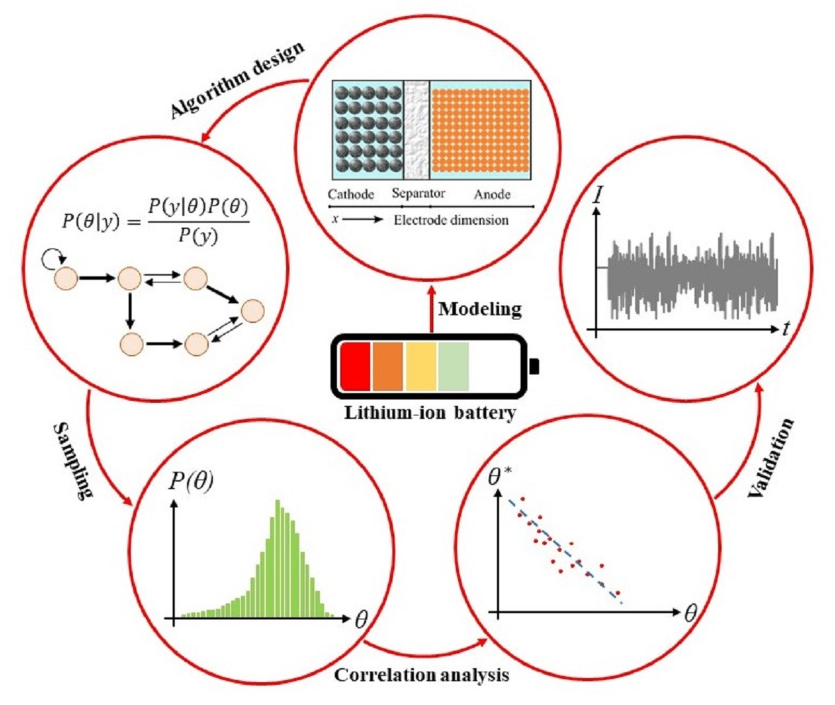
After the parameter estimation has been conducted and the parameters have been selected for validation, two application scenarios each with a time period of three hours are used to validate the parameter estimation results, then the accuracy and effectiveness of the four investigated cases in each scenario are compared. For each case, the parameter values used for validation will be selected according to their identifiability and based on a defined principle, which will be explained in detail later. The load profiles used for the validation and the distribution of the current rate are shown in Figure 2. All lab experiments were conducted in a thermal chamber (Vötsch Industrietechnik GmbH) combined with a battery cycler (CTS, Basytec) under a temperature of 25 °C. The overall workflow for the parameter identification and validation is shown in Figure 3.

4. Results and Discussion

In this section, the parameter sampling results will be shown and discussed, then the estimated parameters will be used to characterize the simulation performance in two application scenarios with highly dynamic load profiles.

4.1. Parameter Distribution

The parameter sampling results are shown in Figure 4. In the following sections, the results for each parameter will be discussed.

Bruggeman coefficients. The posterior distributions of the investigated parameters for the first two cases have a similar form and the parameters have a limited credible interval. As a result, the Bruggeman coefficients in the first two cases can be regarded as practically identifiable. For the third and fourth cases, where the corresponding kinetic and transport parameters measured in the frequency domain with a SOC dependence are substituted, the form of the distribution has changed significantly. The Bruggeman coefficients for the negative electrode and separator show an extended distribution with a much wider credible interval compared to the first two cases. We can first exclude the possibility that the change is caused by the external ohmic resistance, as the parameter identifiability in the first two cases and in the last two cases is similar, respectively. We assume that this change can be attributed to the substituted transport parameters with SOC dependence, which has changed the form of the defined parameter space. It can be concluded here that the substitution of parameters with SOC dependence can have a significant impact on the parameter identifiability.

Solid phase diffusivity. The solid phase diffusivities are only estimated in the first two cases and are substituted as known parameters in the third and fourth cases. In both cases, the PDFs have similar forms. For the negative electrode, the PDFs have a clearly defined lower bound and are approaching the upper bound of the parameter, which is consistent with the fact that the diffusion process with a high diffusivity is no longer rate limiting. Therefore, the solid diffusivity in the anode is assumed to be unidentifiable, where only the lower bound can be determined. In contrast to the anode diffusivity, the cathode diffusivity shows a clearly defined peak for the PDF and a narrow credible interval. Moreover, the diffusivity in the first case is slightly higher than that in the second case. It is worth noticing that the solid phase diffusivity identified using time domain fitting has approximately the same order of magnitude as the value identified in the frequency domain [62], which implies that the diffusivity identified using time domain fitting may be used as an approximated value when a frequency domain based identification is not available.

Liquid phase diffusivity. The liquid phase diffusivity in the first two cases shows a distribution form similar to the solid diffusivity in the anode, where a clearly defined lower bound can be observed but the distribution approaches the upper bound, which leads to a non-rate-limiting behavior. In the third and fourth cases, though a peak can be seen, the credible interval is rather large compared to the parameter bound, thus the liquid diffusivity is practically unidentifiable in all cases. The unidentifiability is possibly attributed to the fact that in fresh cells with nondegraded electrolytes, the overpotential contribution caused by the liquid phase diffusion only amounts to a tiny part of the overall overpotential.

Liquid phase conductivity. The conductivity in the liquid phase can be well identified with a narrow credible interval in the first two cases, the identified values are slightly lower than those identified in the third and fourth cases. In the third and fourth cases, the credible interval becomes significantly wider and the parameter identifiability is lower than in the first two cases, this may imply that the liquid phase conduction is no longer a rate-limiting factor in the model. On the other hand, the distribution form has changed significantly as well, which can be only explained that the parameter space must have been changed by the SOC dependence of the substituted parameters. The phenomenon observed above is consistent with the fact that in fresh cells the liquid phase conduction is generally negligible and cannot be effectively identified.

Solid phase conductivity. The solid phase conductivity in the negative electrode has a wide credible interval and is practically unidentifiable in all cases, which is in line with our expectation that the solid phase conduction process in the anode is usually negligible due to the high conductivity of graphite [73]. The solid phase conductivity in the cathode in the first two cases has a wide credible interval and thus is unidentifiable, while in the third and fourth cases the parameter distribution has a well-defined credible interval and is thus identifiable. It is again worth noticing that the substitution of the SOC-dependent parameters in the model can significantly change the form of the posterior distribution and parameter identifiability irrespective of the external ohmic resistance. The parameter identified in the third case is lower than that in the fourth case by about an order of magnitude, which is very likely caused by the inclusion of the external ohmic resistance in case 4. The estimated solid phase conductivity in the fourth case is close to the value measured using other methods [74], thus we tend to believe that the estimated value is plausible. Another phenomenon worth noticing is that the Bruggeman coefficient of the cathode in case 3 is lower than that in case 4, but the relation for the solid conductivity is reversed. Through a simple calculation, it is found that in both cases the effective solid conductivities in the cathode are nearly the same. By inspecting the equation for the current distribution in the liquid phase, only the effective solid phase conductivity appears and the bulk conductivity does not appear anywhere else. Theoretically, the posterior distribution of the bulk solid conductivity in cathode should give a wide credible interval as in the first two cases, but according to the results, the parameter turns out to be well identifiable. This phenomenon can only be ascribed to the SOC dependence of the substituted parameters. Due to the observed change of the posterior distribution in cases 3 and 4 compared to that in cases 1 and 2, we can basically draw the conclusion that the combined method can indeed change the identifiability of some parameters and obtain more reasonable results.

Interfacial parameters. The three interfacial parameters, namely the kinetic reaction rate constant in both electrodes and the film resistance in the SiC anode, are all unidentifiable in all cases. All PDFs show a credible interval almost comparable with the defined parameter range and a reliable estimation of each parameter is impossible. The results highlight the importance of choosing suitable characterization methods for different model parameters. In most cases, only constant charging/discharging data is selected to establish the identification problem; however, in such cases the current profile generally does not contain any considerable component with a frequency comparable to the characteristic frequency of the interfacial processes, which usually ranges from 100 Hz to 1000 Hz [41,61,75].

From the parameter estimation results and discussions made above, the following conclusions can be made: (1) while the inclusion of the external ohmic resistance may slightly change the probability distribution of the parameters, it basically does not change the identifiability of the parameters; (2) the substitution of identified parameters with SOC dependence may significantly change the posterior distribution of the parameters and identifiability of the parameters; (3) interfacial parameters may be hard or even impossible to identify using the time domain fitting method due to the lack of dynamic current component. The results for the calculated sensitivity indices and credible intervals of the parameters are summarized in

Table 5. Summary of the calculated SI and CI of the parameters.

Parameter	Case 1		Case 2		Case 3		Case 4
	$\mathcal{S}$	CI	$\mathcal{S}$	CI	$\mathcal{S}$	CI	$\mathcal{S}$	CI
${\alpha }_{neg}$	18	[0.50, 0.69]	96	[0.50, 0.53]	5	[0.5, 1.11]	5	[0.50, 1.23]
${\alpha }_{sep}$	5	[2,44, 2.87]	23	[2.77, 2.87]	1	[0.50 2.68]	1	[0.50, 2.71]
${\alpha }_{pos}$	8	[0.72, 1.03]	16	[0.78, 0.94]	4	[0.74, 1.34]	4	[1.15, 1.79]
$D_{s,neg}$ *	16	[−12.19, −12]	22	[−12.13, −12]	-	-	-	-
$D_{s,pos}$ *	14	[−14.08, −13.87]	25	[−14.24, −14.12]	-	-	-	-
$D_{l,0}$ *	6	[−8.63 −8.15]	4	[−8.81, −8.15]	3	[−9.36, −8.29]	4	[−8.92, −8.16]
${\kappa }_{l,0}$ *	7	[−0.26, −0.08]	15	[−0.36, −0.28]	3	[0.03, 0.42]	2	[−0.09 0.41]
${\sigma }_{neg}$ *	1	[0 1.97]	1	[0.05, 2.00]	1	[0, 1.93]	1	[0, 1.95]
${\sigma }_{pos}$ *	1	[−3.07, −0.47]	1	[−3.04, −0.47]	29	[−1.74, −1.65]	9	[−1.06, −0.77]
$R_{f,neg}$ *	1	[−4.91, −1]	1	[−4.99, −1.14]	-	-	-	-
$k_{neg}$ *	1	[−11.97, −9]	1	[−11.94, −9]	-	-	-	-
$k_{pos}$ *	1	[−11.97, −9]	1	[−11.91, −9]	-	-	-	-

* logarithmic scale; CI = 95% credible interval.

.

4.2. Parameter Correlation Analysis

In the last section, the posterior parameter distributions have been characterized, where some parameters show a wide distribution and prove to be unidentifiable. Another important yet unsolved issue is: does any correlation relationship exist among the unidentifiable parameters? In Section 2.3, the principle for the parameter correlation test and the parameter combinations used for the test have been introduced. In this section, the parameter samples will be tested for possible correlation. The results for the sample evaluation are shown in Figure 5, Figure 6, Figure 7, Figure 8 and Figure 9. To infer whether one parameter is possibly correlated with other parameters, the original samples, and the reconstructed sample vectors are plotted on the same axis. To visualize with which processes the tested process is correlated, a parameter correlation chart is generated and shown in Figure 10. In the correlation chart, the number in each column represents the correlation coefficient calculated using Equation (15). Each group of calculated coefficients is scaled by dividing the coefficients by the maximum absolute value of the coefficients in this group so that all values will be transformed into the interval $[-1,1]$ and are comparable.

The parameter correlations for cases 1 and 2 are shown in Figure 5 and Figure 6. It can be observed that in both cases the liquid conduction and diffusion in all electrodes and the solid diffusion in the cathode show an obvious correlation behavior, which indicates that these processes are correlated with other processes. An unexpected result is that the solid conduction process in the cathode and the last three kinetic processes seem not to be correlated with any processes despite that the four parameters corresponding to the four processes have a wide posterior distribution. The solid conduction in the anode is excluded from the investigation here due to the fact that the solid conductivity in the graphite anode is orders of magnitude higher than that in the liquid phase and thus has only negligible contribution to the model output [73]. Berliner et al. [13] investigated the correlation relationship for the diffusion coefficients and reaction rate constant using a synthetic voltage curve and a correlation relationship between $1/k_{neg}$ and $1/k_{pos}$ was discovered. We assume that this correlation may arise from the low current rate used for the experiment. In such cases, the overpotential is less influenced by the diffusion and the fast kinetic processes at the particle–electrolyte interface are dominating. Another possible reason for this unexpected phenomenon is that the correlation relationship in Equation (10) may be distorted by the time-variant concentration in the solid particles and in the electrolyte. Since the correlation has been well observed in the work of Berliner et al. [13], we assume that this could be attributed to the nonuniform liquid phase concentration under 1 C discharging rate. Furthermore, the clearly defined correlation found in [13] may be attributed to the synthetic data generated using a well-defined model.

Figure 5. Results of parameter correlation for case 1. It can be observed that all processes except the conduction in the solid phase, the solid diffusion in the anode, and the interfacial processes are correlated with each other in different parameter ranges.

Figure 5. Results of parameter correlation for case 1. It can be observed that all processes except the conduction in the solid phase, the solid diffusion in the anode, and the interfacial processes are correlated with each other in different parameter ranges.

Figure 6. Results of parameter correlation for case 2. Similar to the results of case 1, it can be observed that all processes except the conduction in the solid phase, the solid diffusion in the anode, and the interfacial processes are correlated with each other in different parameter ranges.

Figure 6. Results of parameter correlation for case 2. Similar to the results of case 1, it can be observed that all processes except the conduction in the solid phase, the solid diffusion in the anode, and the interfacial processes are correlated with each other in different parameter ranges.

To find out whether the unidentifiability arises from the non-sensitivity or correlation relationship of the parameters, the objective function value inside the exponential function in Equation (5) is plotted for both case 1 and case 2 for each possible parameter combination (see Figure 7), the results for case 1 are shown in the upper triangular part of the figure and for case 2 in the lower triangular part. In Figure 7, it can be seen that for case 1 a clearly defined oval isosurface (marked with a red dashed line) can be seen for some parameter combinations, where all parameter combinations inside the ellipse have almost the same objective function value. For the solid conductivity in the cathode, no obvious correlation pattern can be observed, all data points with similar objective function values are concentrated in the region close to the lower bound, which coincides with the posterior distribution. The film resistance is slightly negatively correlated with the anode reaction rate constant. Similarly, a negative correlation is also seen between the anode and cathode reaction constant. Moreover, the found correlation relationship exists only in a limited area of each parameter, for the anode ca. $6\times {10}^{-11}~2\times {10}^{-10}$ ms⁻¹, for the cathode ca. $3\times {10}^{-11}~1\times {10}^{-10}$ ms⁻¹, which corresponds to the peak area in the posterior distribution for both parameters (see Figure 4). An obvious positive correlation can be observed between the cathode reaction constant and the film resistance. This may be caused by the coordinated change of the charge transfer overpotential between the anode and cathode. The phenomena shown above indicate that the investigations and conclusions made using synthetic data may not be valid in practical applications, which highlights the necessity of a comprehensive parameter identifiability analysis in practical applications.

Figure 7. Two-dimensional plot of the objective function value for case 1 (upper triangular) and case 2 (lower triangular). For case 1, an obvious correlation can be observed between the film resistance and the anodic reaction rate constant, film resistance and the cathodic reaction rate constant, and anodic reaction rate constant and cathodic reaction rate constant. For case 2, no correlation pattern can be seen.

Figure 7. Two-dimensional plot of the objective function value for case 1 (upper triangular) and case 2 (lower triangular). For case 1, an obvious correlation can be observed between the film resistance and the anodic reaction rate constant, film resistance and the cathodic reaction rate constant, and anodic reaction rate constant and cathodic reaction rate constant. For case 2, no correlation pattern can be seen.

For case 2, it can be seen that no clearly defined isoline or isosurface is existent for any parameter combination, and all global optimum points are nearly evenly distributed. This phenomenon may have two origins: (1) the isoline or isosurface lies outside the defined parameter range and cannot be observed here; (2) these parameters have only negligible influence on the model output.

For cases 3 and 4, similar behavior can be observed in Figure 8 and Figure 9. For all processes except for the solid conduction in the anode, a good correlation can be observed. The solid conduction in the anode is not well correlated with other processes, we assume that this is attributable to the higher conductivity and negligible overpotential caused by the graphite anode. According to Figure 10c,d, all processes investigated in the correlation chart are correlated and a unique optimal parameter combination does not exist. It is worth mentioning here that although the solid conduction in the cathode shows a correlation relationship with other processes, the solid conductivity in the cathode has a narrow credible interval (see Figure 4) and is thus regarded as identifiable.

Figure 8. Results of parameter correlation for case 3. A correlation relation can be observed for each process except for the solid conduction in the anode.

Figure 8. Results of parameter correlation for case 3. A correlation relation can be observed for each process except for the solid conduction in the anode.

Figure 9. Results of parameter correlation for case 4. A correlation relation can be observed for each process except for the solid conduction in the anode.

Figure 9. Results of parameter correlation for case 4. A correlation relation can be observed for each process except for the solid conduction in the anode.

Figure 10. Correlation chart for cases 1–4, where each column in the matrix represents the correlation coefficients with the tested process.

Figure 10. Correlation chart for cases 1–4, where each column in the matrix represents the correlation coefficients with the tested process.

4.3. Selection of Parameters from Posterior Distributions

In previous sections, a comprehensive identifiability and correlation analysis has been conducted, the results have been shown and explained in detail. However, the resulting parameter distributions cannot be used as the input for the p2D model to validate the results; therefore, a point estimate must be selected from the posterior distributions. For the experimental validation, generally the expected value of each parameter is chosen and substituted into the model [10]. Nevertheless, the prerequisite for selecting the expected value as the point estimate is that either all parameters are not correlated or they are only simply linearly correlated so that for the expected values the linear correlation relationship is still valid. For example, if we assume that the parameters ${\theta }_1$ and ${\theta }_2$ are linearly correlated and the following relation holds:

$${\theta }_1=\alpha {\theta }_2+\beta$$

(18)

where $\alpha$ and $\beta$ are correlation constants. If the expected value operator is applied to both sides of Equation (18), the following equation is obtained:

$$E\left[{\theta }_1\right]=\alpha E\left[{\theta }_2\right]+\beta$$

(19)

which implies that for both ${\theta }_1$ and ${\theta }_2$ the expected value can be selected as the point estimate. However, if ${\theta }_1$ and ${\theta }_2$ are not linearly but instead nonlinearly correlated, for example:

$${\theta }_1=\frac{\alpha }{{\theta }_2}+\beta$$

(20)

and then the expected value operator is again applied to both sides of the equation, the following equation can be obtained:

$$E\left[{\theta }_1\right]=\alpha E\left[\frac{1}{{\theta }_2}\right]+\beta \ne \alpha \frac{1}{E\left[{\theta }_2\right]}+\beta$$

(21)

This equation clearly indicates that if the parameters are not linearly correlated, the expected values of the parameters will not fulfill the correlation relationship. Simply selecting the expected value for each correlated parameter may lead to an unexpected error. In this work, the parameter combination used for the experimental validation will be selected according to the following principle:

• For parameters with a small credible interval (irrespective of identifiability), the expected value is selected.
• For parameters that are practically unidentifiable and there exists no correlation with other parameters, the expected value is selected.
• For parameters that are correlated, the expected value of the parameter with the highest sensitivity index will be calculated and selected for validation, the values of other parameters will be determined accordingly so that the correlation among the chosen parameters is still valid. If multiple parameter combinations are possible, then the combination closest to the expected values is chosen.

According to the principles explained above, the determined parameter values are summarized in

Table 6. Summary of the parameter values selected for the validation test.

Parameter	Scale	Case 1	Case 2	Case 3	Case 4
${\alpha }_{neg}$	linear	0.554	0.511	0.753	0.870
${\alpha }_{sep}$	linear	2.736	2.843	1.256	2.756
${\alpha }_{pos}$	linear	0.865	0.863	0.801	1.105
$D_{s,neg}$	log	−12.059	−12.042	-	-
$D_{s,pos}$	log	−13.986	−14.188	-	-
$D_{l,0}$	log	−8.323	−8.386	−8.964	−9.092
${\kappa }_{l,0}$	log	−0.190	−0.327	0.068	0.064
${\sigma }_{neg}$	log	0.531	1.967	0.729	0.793
${\sigma }_{pos}$	log	−2.447	−1.809	−1.696	−0.920
$R_{f,neg}$	log	−2.533	−3.661	-	-
$k_{neg}$	log	−10.191	−10.352	-	-
$k_{pos}$	log	−10.595	−9.118	-	-

.

4.4. Validation with Dynamic Load Profile

The results for the parameter validation with the two application scenarios are shown in Figure 11. In scenario 1, it can be observed that the full model without external ohmic resistance achieves the worst simulation performance, where the maximum error reaches about 400 mV and the root-mean-square error (RMSE) is calculated to be 124.7 mV. The voltage window of the investigated cell is between 2.5 V and 4.2 V, if the OCV curve is approximated with a straight line, then an RMSE of 124.7 mV corresponds to a 7.3% average SOC error, which is unacceptable for a state estimation application. Although in all cases the parameters are identified with the same discharging profile and the best objective function values are almost the same and show no qualitative difference, the most primitive model, namely where all parameters are fitted at the same time and without considering the external ohmic resistance, shows an unacceptable error and fails to model the dynamic operation. The results for the full model with the external ohmic resistance become much better with an RMSE of 35.8 mV, the error is below 100 mV at most times, but a maximum error of about 200 mV can still be seen. The combined model without the external ohmic resistance achieves a qualitative improvement, the RMSE is 17.4 mV and corresponds to a 1% average SOC error, assuming a linear relationship between the cell voltage (2.5~4.2 V) and the SOC (0~100%). The combined model with the external ohmic resistance achieves the best performance with an RMSE of only 12.6 mV, corresponding to a 0.7% average SOC error.

The results for scenario 2 are similar to that in scenario 1 and the error in all cases is slightly lower, again the combined model with external resistance achieves the lowest error, thus justifying the application of the combined procedure for parameter identification. To have an overall comparison of the simulation performance for the four cases, the root-mean-square error (RMSE) has been calculated and listed in

Table 7. Calculated RMSE values for the validation of each case.

RMSE (mV)	Case 1	Case 2	Case 3	Case 4
scenario 1	124.7	35.8	17.4	12.6
scenario 2	117.8	31.7	16.1	11.8

.

5. Conclusions and Outlooks

In this present work, parameter identifiability with the p2D model in four cases is investigated and analyzed: models with or without external ohmic resistance, a model with all chosen parameters fitted, and a model where the kinetic parameters determined in the frequency domain are substituted (combined model). The results of the parameter space sampling indicate that the external ohmic resistance has a considerable impact on the parameter identifiability, especially on the bulk conductivity in the solid and liquid phases, while the results for the Bruggeman coefficients in each electrode layer only show small differences. In the first two cases, all interface parameters are practically unidentifiable. For the third and fourth cases, where the values for the kinetic parameters determined using the EIS are substituted, the parameter identifiability results have changed. Though the Bruggeman coefficients still cannot be uniquely identified, the bulk conductivities in the liquid phase and solid conductivity in the cathode are significantly better compared with the values determined using different methods from the literature.

The parameter correlation analysis indicates that the ohmic conduction and diffusion processes in the solid and liquid phases are generally correlated, given the constant discharging profile used for the parameter identifiability analysis. The only parameter that can be identified while considering the external ohmic resistance and the SOC dependence is the solid conductivity in the cathode. Therefore, it is worth mentioning again that although the constant charging/discharging voltage profile can be easily fitted using a properly chosen nonlinear optimization algorithm to extract some physicochemical parameter values, the reliability and uniqueness of the results are usually problematic.

Then the estimated parameters are substituted into the p2D model and validated with two highly dynamic load profiles and the simulation results are compared with the experimentally measured voltage response. The results again confirm that the combined model with the external ohmic resistance performs the best and achieves an RMSE on the level of 12 mV. To sum up, the combined type model with both the time domain and frequency domain method clearly outperforms other model types investigated in this work and achieves the best RMSE even when the model is simulated with a highly dynamic profile.

Based on the analysis and conclusions made before, we suggest that the kinetic parameters such as the reaction rate constants and diffusion coefficients should be estimated using frequency domain methods. A carefully selected dynamic voltage and current profile should be used for the parameter identification in the time domain if only the time domain fitting is used for the parameter identification. The dynamic profiles should at least include the characteristic frequency components of the corresponding processes and parameters. Furthermore, we assume that with carefully designed current profiles some of the currently unidentifiable parameters may become identifiable.

References

- Masoudi, R.; Uchida, T.; McPhee, J. Parameter estimation of an electrochemistry-based lithium-ion battery model. J. Power Sources 2015, 291, 215–224. [Google Scholar] [CrossRef] [Green Version]
- Miniguano, H.; Barrado, A.; Lázaro, A.; Zumel, P.; Fernández, C. General parameter identification procedure and comparative study of Li-Ion battery models. IEEE Trans. Veh. Technol. 2019, 69, 235–245. [Google Scholar] [CrossRef]
- Wimarshana, B.; Bin-Mat-Arishad, I.; Fly, A. Parameter sensitivity analysis of a physico-chemical lithium-ion battery model with combined discharge voltage and electrochemical impedance data. J. Power Sources 2022, 527, 231125. [Google Scholar] [CrossRef]
- Laue, V.; Röder, F.; Krewer, U. Practical identifiability of electrochemical P2D models for lithium-ion batteries. J. Appl. Electrochem. 2021, 51, 1253–1265. [Google Scholar] [CrossRef]
- Lai, X.; Gao, W.; Zheng, Y.; Ouyang, M.; Li, J.; Han, X.; Zhou, L. A comparative study of global optimization methods for parameter identification of different equivalent circuit models for Li-ion batteries. Electrochim. Acta 2019, 295, 1057–1066. [Google Scholar] [CrossRef]
- Tran, M.K.; DaCosta, A.; Mevawalla, A.; Panchal, S.; Fowler, M. Comparative study of equivalent circuit models performance in four common lithium-ion batteries: LFP, NMC, LMO, NCA. Batteries 2021, 7, 51. [Google Scholar] [CrossRef]
- Uddin, K.; Picarelli, A.; Lyness, C.; Taylor, N.; Marco, J. An acausal Li-ion battery pack model for automotive applications. Energies 2014, 7, 5675–5700. [Google Scholar] [CrossRef]
- Uddin, K.; Perera, S.; Widanage, W.D.; Marco, J. Characterising Li-ion battery degradation through the identification of perturbations in electrochemical battery models. World Electr. Veh. J. 2015, 7, 76–84. [Google Scholar] [CrossRef] [Green Version]
- Yang, X.; Chen, L.; Xu, X.; Wang, W.; Xu, Q.; Lin, Y.; Zhou, Z. Parameter identification of electrochemical model for vehicular lithium-ion battery based on particle swarm optimization. Energies 2017, 10, 1811. [Google Scholar] [CrossRef] [Green Version]
- Brady, N.W.; Gould, C.A.; West, A.C. Quantitative parameter estimation, model selection, and variable selection in battery science. J. Electrochem. Soc. 2019, 167, 013501. [Google Scholar] [CrossRef]
- Rahman, M.A.; Anwar, S.; Izadian, A. Electrochemical model parameter identification of a lithium-ion battery using particle swarm optimization method. J. Power Sources 2016, 307, 86–97. [Google Scholar] [CrossRef]
- Forman, J.C.; Moura, S.J.; Stein, J.L.; Fathy, H.K. Genetic identification and fisher identifiability analysis of the Doyle–Fuller–Newman model from experimental cycling of a LiFePO4 cell. J. Power Sources 2012, 210, 263–275. [Google Scholar] [CrossRef]
- Berliner, M.D.; Zhao, H.; Das, S.; Forsuelo, M.; Jiang, B.; Chueh, W.H.; Bazant, M.Z.; Braatz, R.D. Nonlinear Identifiability Analysis of the Porous Electrode Theory Model of Lithium-Ion Batteries. J. Electrochem. Soc. 2021, 168, 090546. [Google Scholar] [CrossRef]
- Rajabloo, B.; Jokar, A.; Désilets, M.; Lacroix, M. An inverse method for estimating the electrochemical parameters of lithium-ion batteries. J. Electrochem. Soc. 2016, 164, A99. [Google Scholar] [CrossRef]
- Pozzi, A.; Ciaramella, G.; Volkwein, S.; Raimondo, D.M. Optimal design of experiments for a lithium-ion cell: Parameters identification of an isothermal single particle model with electrolyte dynamics. Ind. Eng. Chem. Res. 2018, 58, 1286–1299. [Google Scholar] [CrossRef] [Green Version]
- Jin, N.; Danilov, D.L.; Van den Hof, P.M.; Donkers, M. Parameter estimation of an electrochemistry-based lithium-ion battery model using a two-step procedure and a parameter sensitivity analysis. Int. J. Energy Res. 2018, 42, 2417–2430. [Google Scholar] [CrossRef] [Green Version]
- Li, J.; Wang, L.; Lyu, C.; Liu, E.; Xing, Y.; Pecht, M. A parameter estimation method for a simplified electrochemical model for Li-ion batteries. Electrochim. Acta 2018, 275, 50–58. [Google Scholar] [CrossRef]
- Gopalakrishnan, K.; Offer, G.J. A Composite Single Particle Lithium-ion Battery Model through System Identification. IEEE Trans. Control Syst. Technol. 2021, 30, 1–13. [Google Scholar] [CrossRef]
- Deng, Z.; Deng, H.; Yang, L.; Cai, Y.; Zhao, X. Implementation of reduced-order physics-based model and multi-parameters identification strategy for lithium-ion battery. Energy 2017, 138, 509–519. [Google Scholar] [CrossRef]
- Kosch, S.; Zhao, Y.; Sturm, J.; Schuster, J.; Mulder, G.; Ayerbe, E.; Jossen, A. A computationally efficient multi-scale model for lithium-ion cells. J. Electrochem. Soc. 2018, 165, A2374. [Google Scholar] [CrossRef]
- Wu, L.; Pang, H.; Geng, Y.; Liu, X.; Liu, J.; Liu, K. Low-complexity state of charge and anode potential prediction for lithium-ion batteries using a simplified electrochemical model-based observer under variable load condition. Int. J. Energy Res. 2022, 46, 11834–11848. [Google Scholar] [CrossRef]
- Ding, Q.; Wang, Y.; Chen, Z. Parameter identification of reduced-order electrochemical model simplified by spectral methods and state estimation based on square-root cubature Kalman filter. J. Energy Storage 2022, 46, 103828. [Google Scholar] [CrossRef]
- Kalogiannis, T.; Hosen, M.S.; Sokkeh, M.A.; Goutam, S.; Jaguemont, J.; Jin, L.; Qiao, G.; Berecibar, M.; Van Mierlo, J. Comparative Study on Parameter Identification Methods for Dual-Polarization Lithium-Ion Equivalent Circuit Model. Energies 2019, 12, 4031. [Google Scholar] [CrossRef] [Green Version]
- De Levie, R. On porous electrodes in electrolyte solutions: I. Capacitance effects. Electrochim. Acta 1963, 8, 751–780. [Google Scholar] [CrossRef]
- De Levie, R. On porous electrodes in electrolyte solutions—IV. Electrochim. Acta 1964, 9, 1231–1245. [Google Scholar] [CrossRef]
- Vyroubal, P.; Kazda, T. Equivalent circuit model parameters extraction for lithium ion batteries using electrochemical impedance spectroscopy. J. Energy Storage 2018, 15, 23–31. [Google Scholar] [CrossRef]
- Choi, W.; Shin, H.C.; Kim, J.M.; Choi, J.Y.; Yoon, W.S. Modeling and Applications of Electrochemical Impedance Spectroscopy (EIS) for Lithium-ion Batteries. J. Electrochem. Sci. Technol. 2020, 11, 1–13. [Google Scholar] [CrossRef] [Green Version]
- Illig, J.; Ender, M.; Weber, A.; Ivers-Tiffée, E. Modeling graphite anodes with serial and transmission line models. J. Power Sources 2015, 282, 335–347. [Google Scholar] [CrossRef]
- Bizeray, A.M.; Kim, J.H.; Duncan, S.R.; Howey, D.A. Identifiability and parameter estimation of the single particle lithium-ion battery model. IEEE Trans. Control Syst. Technol. 2018, 27, 1862–1877. [Google Scholar] [CrossRef] [Green Version]
- Dokko, K.; Mohamedi, M.; Fujita, Y.; Itoh, T.; Nishizawa, M.; Umeda, M.; Uchida, I. Kinetic characterization of single particles of LiCoO2 by AC impedance and potential step methods. J. Electrochem. Soc. 2001, 148, A422. [Google Scholar] [CrossRef]
- Prasad, G.K.; Rahn, C.D. Reduced order impedance models of lithium ion batteries. J. Dyn. Syst. Meas. Control 2014, 136, 041012. [Google Scholar] [CrossRef]
- Sikha, G.; White, R.E. Analytical expression for the impedance response of an insertion electrode cell. J. Electrochem. Soc. 2006, 154, A43. [Google Scholar] [CrossRef]
- Sikha, G.; White, R.E. Analytical expression for the impedance response for a lithium-ion cell. J. Electrochem. Soc. 2008, 155, A893. [Google Scholar] [CrossRef] [Green Version]
- Murbach, M.D.; Schwartz, D.T. Extending Newman’s pseudo-two-dimensional lithium-ion battery impedance simulation approach to include the nonlinear harmonic response. J. Electrochem. Soc. 2017, 164, E3311. [Google Scholar] [CrossRef]
- Zhou, X.; Huang, J. Impedance-Based diagnosis of lithium ion batteries: Identification of physical parameters using multi-output relevance vector regression. J. Energy Storage 2020, 31, 101629. [Google Scholar] [CrossRef]
- Lasia, A. Electrochemical impedance spectroscopy and its applications. In Modern Aspects of Electrochemistry; Springer: Berlin/Heidelberg, Germany, 2002; pp. 143–248. [Google Scholar]
- Boukamp, B.A. Distribution (function) of relaxation times, successor to complex nonlinear least squares analysis of electrochemical impedance spectroscopy? J. Electrochem. Soc. 2020, 2, 042001. [Google Scholar] [CrossRef]
- Danzer, M.A. Generalized Distribution of Relaxation Times Analysis for the Characterization of Impedance Spectra. Batteries 2019, 5, 53. [Google Scholar] [CrossRef] [Green Version]
- Hahn, M.; Schindler, S.; Triebs, L.C.; Danzer, M.A. Optimized Process Parameters for a Reproducible Distribution of Relaxation Times Analysis of Electrochemical Systems. Batteries 2019, 5, 43. [Google Scholar] [CrossRef] [Green Version]
- Gavrilyuk, A.L.; Osinkin, D.A.; Bronin, D.I. On a variation of the Tikhonov regularization method for calculating the distribution function of relaxation times in impedance spectroscopy. Electrochim. Acta 2020, 354, 136683. [Google Scholar] [CrossRef]
- Shafiei Sabet, P.; Warnecke, A.J.; Meier, F.; Witzenhausen, H.; Martinez-Laserna, E.; Sauer, D.U. Non-invasive yet separate investigation of anode/cathode degradation of lithium-ion batteries (nickel–cobalt–manganese vs. graphite) due to accelerated aging. J. Power Sources 2020, 449, 227369. [Google Scholar] [CrossRef]
- Ivers-Tiffee, E.; Weber, A. Evaluation of electrochemical impedance spectra by the distribution of relaxation times. J. Ceram. Soc. Jpn. 2017, 125, 193–201. [Google Scholar] [CrossRef] [Green Version]
- Boukamp, B.A.; Rolle, A. Analysis and application of distribution of relaxation times in solid state ionics. Solid State Ionics 2017, 302, 12–18. [Google Scholar] [CrossRef]
- Boukamp, B.A.; Rolle, A. Use of a distribution function of relaxation times (DFRT) in impedance analysis of SOFC electrodes. Solid State Ionics 2018, 314, 103–111. [Google Scholar] [CrossRef]
- Rolle, A.; Mohamed, H.A.A.; Huo, D.; Capoen, E.; Mentre, O.; Vannier, R.N.; Daviero-Minaud, S.; Boukamp, B.A. Ca3Co4O9+δ, a growing potential SOFC cathode material: Impact of the layer composition and thickness on the electrochemical properties. Solid State Ionics 2016, 294, 21–30. [Google Scholar] [CrossRef]
- Illig, J.; Ender, M.; Chrobak, T.; Schmidt, J.P.; Klotz, D.; Ivers-Tiffée, E. Separation of charge transfer and contact resistance in LiFePO4-cathodes by impedance modeling. J. Electrochem. Soc. 2012, 159, A952. [Google Scholar] [CrossRef]
- Illig, J.; Schmidt, J.P.; Weiss, M.; Weber, A.; Ivers-Tiffée, E. Understanding the impedance spectrum of 18650 LiFePO4-cells. J. Power Sources 2013, 239, 670–679. [Google Scholar] [CrossRef]
- Doyle, M.; Fuller, T.F.; Newman, J. Modeling of galvanostatic charge and discharge of the lithium/polymer/insertion cell. J. Electrochem. Soc. 1993, 140, 1526. [Google Scholar] [CrossRef]
- Doyle, M.; Newman, J. Modeling the performance of rechargeable lithium-based cells: Design correlations for limiting cases. J. Power Sources 1995, 54, 46–51. [Google Scholar] [CrossRef]
- Doyle, M.; Newman, J.; Gozdz, A.S.; Schmutz, C.N.; Tarascon, J.M. Comparison of modeling predictions with experimental data from plastic lithium ion cells. J. Electrochem. Soc. 1996, 143, 1890–1903. [Google Scholar] [CrossRef]
- Iooss, B.; Lemaître, P. A review on global sensitivity analysis methods. In Uncertainty Management in Simulation-Optimization of Complex Systems; Springer: Berlin/Heidelberg, Germany, 2015; pp. 101–122. [Google Scholar]
- Sobol, I.M. Global sensitivity indices for nonlinear mathematical models and their Monte Carlo estimates. Math. Comput. Simul. 2001, 55, 271–280. [Google Scholar] [CrossRef]
- Kumbhare, S.; Shahmoradi, A. MatDRAM: A pure-MATLAB Delayed-Rejection Adaptive Metropolis-Hastings Markov Chain Monte Carlo Sampler. arXiv 2020, arXiv:2010.04190. [Google Scholar]
- Gelman, A.; Gilks, W.R.; Roberts, G.O. Weak convergence and optimal scaling of random walk Metropolis algorithms. Ann. Appl. Probab. 1997, 7, 110–120. [Google Scholar] [CrossRef]
- Rabissi, C.; Innocenti, A.; Sordi, G.; Casalegno, A. A Comprehensive Physical-Based Sensitivity Analysis of the Electrochemical Impedance Response of Lithium-Ion Batteries. Energy Technol. 2021, 9, 2000986. [Google Scholar] [CrossRef]
- Astrom, K.; Bellman, R. On structural identifiability. Math. Biosci. 1970, 7, 329–339. [Google Scholar]
- Meyers, J.P.; Doyle, M.; Darling, R.M.; Newman, J. The impedance response of a porous electrode composed of intercalation particles. J. Electrochem. Soc. 2000, 147, 2930. [Google Scholar] [CrossRef]
- Schönleber, M.; Uhlmann, C.; Braun, P.; Weber, A.; Ivers-Tiffée, E. A consistent derivation of the impedance of a lithium-ion battery electrode and its dependency on the state-of-charge. Electrochim. Acta 2017, 243, 250–259. [Google Scholar] [CrossRef]
- Nyman, A.; Zavalis, T.G.; Elger, R.; Behm, M.; Lindbergh, G. Analysis of the polarization in a Li-ion battery cell by numerical simulations. J. Electrochem. Soc. 2010, 157, A1236. [Google Scholar] [CrossRef]
- Reimers, J.N. Accurate and efficient treatment of foil currents in a spiral wound Li-ion cell. J. Electrochem. Soc. 2013, 161, A118. [Google Scholar] [CrossRef]
- Zhao, Y.; Kumtepeli, V.; Ludwig, S.; Jossen, A. Investigation of the distribution of relaxation times of a porous electrode using a physics-based impedance model. J. Power Sources 2022, 530, 231250. [Google Scholar] [CrossRef]
- Zhao, Y.; Kücher, S.; Jossen, A. Investigation of the Diffusion Phenomena in Lithium-ion Batteries with Distribution of Relaxation Times. Electrochim. Acta 2022, 432, 141174. [Google Scholar] [CrossRef]
- Sturm, J.; Rheinfeld, A.; Zilberman, I.; Spingler, F.B.; Kosch, S.; Frie, F.; Jossen, A. Modeling and simulation of inhomogeneities in a 18650 nickel-rich, silicon-graphite lithium-ion cell during fast charging. J. Power Sources 2019, 412, 204–223. [Google Scholar] [CrossRef] [Green Version]
- Chen, C.H.; Planella, F.B.; O’regan, K.; Gastol, D.; Widanage, W.D.; Kendrick, E. Development of experimental techniques for parameterization of multi-scale lithium-ion battery models. J. Electrochem. Soc. 2020, 167, 080534. [Google Scholar] [CrossRef]
- Tang, S.; Wang, Z.; Guo, H.; Wang, J.; Li, X.; Yan, G. Systematic parameter acquisition method for electrochemical model of 4.35 V LiCoO2 batteries. Solid State Ionics 2019, 343, 115083. [Google Scholar] [CrossRef]
- Wei, Y.; Zheng, J.; Cui, S.; Song, X.; Su, Y.; Deng, W.; Wu, Z.; Wang, X.; Wang, W.; Rao, M.; et al. Kinetics tuning of Li-ion diffusion in layered Li (NixMnyCoz) O2. J. Am. Chem. Soc. 2015, 137, 8364–8367. [Google Scholar] [CrossRef] [PubMed]
- Noh, H.J.; Youn, S.; Yoon, C.S.; Sun, Y.K. Comparison of the structural and electrochemical properties of layered Li [NixCoyMnz] O2 (x = 1/3, 0.5, 0.6, 0.7, 0.8 and 0.85) cathode material for lithium-ion batteries. J. Power Sources 2013, 233, 121–130. [Google Scholar] [CrossRef]
- Landesfeind, J.; Gasteiger, H.A. Temperature and concentration dependence of the ionic transport properties of lithium-ion battery electrolytes. J. Electrochem. Soc. 2019, 166, A3079. [Google Scholar] [CrossRef]
- Richardson, G.; Foster, J.M.; Sethurajan, A.K.; Krachkovskiy, S.A.; Halalay, I.C.; Goward, G.R.; Protas, B. The effect of ionic aggregates on the transport of charged species in lithium electrolyte solutions. J. Electrochem. Soc. 2018, 165, H561. [Google Scholar] [CrossRef]
- Krachkovskiy, S.A.; Bazak, J.D.; Fraser, S.; Halalay, I.C.; Goward, G.R. Determination of mass transfer parameters and ionic association of LiPF6: Organic carbonates solutions. J. Electrochem. Soc. 2017, 164, A912. [Google Scholar] [CrossRef]
- Farkhondeh, M.; Safari, M.; Pritzker, M.; Fowler, M.; Han, T.; Wang, J.; Delacourt, C. Full-range simulation of a commercial LiFePO4 electrode accounting for bulk and surface effects: A comparative analysis. J. Electrochem. Soc. 2013, 161, A201. [Google Scholar] [CrossRef]
- Prada, E.; Di Domenico, D.; Creff, Y.; Bernard, J.; Sauvant-Moynot, V.; Huet, F. Simplified electrochemical and thermal model of LiFePO4-graphite Li-ion batteries for fast charge applications. J. Electrochem. Soc. 2012, 159, A1508. [Google Scholar] [CrossRef] [Green Version]
- Park, M.; Zhang, X.; Chung, M.; Less, G.B.; Sastry, A.M. A review of conduction phenomena in Li-ion batteries. J. Power Sources 2010, 195, 7904–7929. [Google Scholar] [CrossRef]
- Wang, S.; Yan, M.; Li, Y.; Vinado, C.; Yang, J. Separating electronic and ionic conductivity in mix-conducting layered lithium transition-metal oxides. J. Power Sources 2018, 393, 75–82. [Google Scholar] [CrossRef]
- Shafiei Sabet, P.; Sauer, D.U. Separation of predominant processes in electrochemical impedance spectra of lithium-ion batteries with nickel-manganese-cobalt cathodes. J. Power Sources 2019, 425, 121–129. [Google Scholar] [CrossRef]
Figure 1.
The two scenarios where the corresponding processes/parameters are unidentifiable with (a) overlapping peaks and (b) one peak of a negligible polarization resistance.
Figure 2.
Dynamic load profile used for the validation of parameter estimation. (a) current profile; (b) distribution of the current rate.
Figure 3.
Workflow for the parameter identification and validation conducted in the present work. The different colors in the simulation results and error analysis sections represent the results of different test cases.
Figure 4.
Probability distribution of the sampled parameters in the four cases. The probability density distribution function (PDF) is shown with the histogram and the cumulative distribution function (CDF) for each PDF is shown with a dashed line using the same color as the PDF.
Figure 11.
Validation results for for all cases with (a) the voltage profile in scenario 1, (b) voltage error in scenario 1, (c) voltage profile in scenario 2, and (d) voltage error in scenario 2.