
Analysis of Tandem Queue with Multi-Server Stages and Group Service at the Second Stage


Department of Applied Mathematics and Computer Science, Belarusian State University, 4, Nezavisimosti Ave., 220030 Minsk, Belarus
*
Author to whom correspondence should be addressed.
Axioms 2024, 13(4), 214; https://doi.org/10.3390/axioms13040214
Submission received: 19 February 2024
/
Revised: 14 March 2024
/
Accepted: 22 March 2024
/
Published: 25 March 2024
(This article belongs to the Special Issue Advances in Stochastic Processes and Stochastic Differential Equations)
Abstract
:In this paper, we consider a tandem dual queuing system consisting of multi-server stages. Stage 1 is characterized by an infinite buffer, one-by-one service of customers, and an exponential distribution of service times. Stage 2 is characterized by a finite buffer and a phase-type distribution of service times. Service at Stage 2 is provided to groups of customers. The service time of a group depends on the size of the group. The size is restricted by two thresholds. The waiting time of a customer at each stage is limited by a random variable with an exponential distribution, with the parameter depending on the stage. After service at Stage 1, a customer can depart from the system or try to enter Stage 2. If the buffer at this stage is full, the customer is either lost or returns for service at Stage 1. Customer arrivals are described by the versatile Markov arrival process. The system is studied via consideration of a multi-dimensional continuous-time Markov chain. Numerical examples, which highlight the influence of the thresholds on the system performance measures, are presented. The possibility of solving optimization problems is illustrated.
MSC:
60K25; 60K30; 68M20; 90B221. Introduction
Tandem queues are useful for modeling the operation of various telecommunication, logistic, production, manufacturing, and other systems and networks, and the existing literature is very extensive; see, e.g., [1,2,3,4,5,6]. The work in [2,3,4,5] gives extensive surveys of the state-of-the-art in analysis of tandem queues. In [1] by M. Neuts, the comprehensive analysis of a two-server tandem queue with the stationary Poisson arrival process, general service time distribution of service times at the first stage of the tandem, exponential service time distribution at the second stage and a finite intermediate buffer are implemented. This tandem queuing system is studied in terms of an embedded semi-Markov process. The presented analysis is quite complicated, aiming to implement analysis of tandem queues with a more complicated arrival process and more general distribution of the service time at the second stage (at the expense of considering less general distribution of service time at the first stage). Further, M. Neuts developed the matrix analytic method. This method allows us to effectively treat various complicated tandem queues. In this paper, essentially we use that method. In [6], a similar methodology was applied for the study of a tandem queue with two stages, the Markov arrival process () of customers, and finite buffers and phase type distribution of the service time at both stages of the tandem.
A brief survey of the relevant literature and examples of potential applications of tandem queues with group service, which are similar to what is considered in this paper, to the analysis and optimization of real systems in service, production and manufacturing sectors can be found in the recent paper [7]. As it is highlighted in [7], two of the most distinguishing features of the model considered in that paper are as follows:
(a) The arrival flow is described not by the stationary Poisson process, as in the overwhelming majority of existing papers, but by the Markov arrival process () which is much more complicated but suitable for taking into account such typical features of the arrival processes as possible fluctuation of the instantaneous arrival rate, over-dispersion (large variance of inter-arrival times) and positive correlation of successive inter-arrival times. The neglect to take these features into account causes huge errors in the prediction of performance measures for the system. Predicted results based on the model of the stationary Poisson arrival process are too optimistic. For example, for the single server queuing model with a finite buffer the probability of a customer loss due to the buffer overflow, computed in assumption that the arrival flow is described by the stationary Poisson arrival process, can be of order . The value of this probability computed with the use of the as the model of arrival flow with the same mean arrival rate and even relatively small (about 0.2) positive correlation of the neighboring inter-arrival times is about The same order of this probability is obtained via the computer simulation of the system. Similar increase of the loss probability occurs when the coefficient of variation of inter-arrival times is large. The reason for this phenomenon is the following. If the inter-arrival times are positively correlated, then periods of time, during which customers arrive rarely (and the bandwidth of the server is under-utilized, the server often stays idle) alternate with periods of time during which customers arrive frequently (and a lot of arriving customers are lost). The same occurs when the inter-arrival times have a large variance.
(b) Service at Stage 2 is provided only to groups of customers. This is typical for many real systems, in particular production, delivery, and transportation systems. In transportation systems, the lower limit of a group size is defined by economic considerations (to avoid service by almost empty vehicles). The upper limit is defined by the capacity of the exploited service vehicle (airplane, ship, bus, train, etc.). The task of choosing these limits is non-trivial. The small value of the lower limit helps to avoid leaving servers idle in the presence of a queue. But the potential profit from using the group service (smaller service time per customer) is poorly used. A large value of the lower limit helps to use the advantages of a group service to a greater extent but leads to a longer waiting time for customers until the group of the minimal size required for the service beginning is accumulated.
Results of the analysis of tandem queues with the group service of customers, in particular, the tandem queue considered in [7], can be used for the optimal choice of the limits of a group size and optimal planning of the fleet of vehicles of a transportation company that has the opportunity to match the capacity of the provided service vehicle to the size of the waiting group of customers.
It is worth mentioning that a significant contribution to the study of isolated queues with group customer service was made by S. Chakravarthy; see, e.g., [8,9,10,11,12,13]. Mention also the papers [14,15,16,17]. In [14,15,16], the process or its generalizations is supposed. In [17], dependence of a group service time on its size is examined and applications to fog and cloud computing systems are discussed.
The main advantage of the tandem queue considered in this paper, in comparison to the rather advanced model considered in [7], is that both stages of a tandem considered in [7] are described by the single-server systems, while we assume that they are multi-server systems. This advantage is essential both from the theoretical and practical points of view. From the former one, it is known that due to the description by a more complicated random process, analysis of multi-server queues may be considerably more difficult than the study of single-server queues. From the practical point of view, this is important because in many companies customer’s service technological process consists of two stages: auxiliary and essential. The number of servers at Stage 1 providing auxiliary services such as registration of customers, their preparation for service, order picking, packing, passengers boarding, etc., and the number of servers at Stage 2 that provide the essential service (e.g., the number of vehicles implementing orders delivering, cars, buses, trains, aircrafts, etc., and implementing passengers transportation, etc.,) is more than one. Another two distinctions of the models considered here and in [7] are as follows. Here, we assume that, with an arbitrarily fixed probability, an arbitrary customer can depart from the tandem after service at Stage 1. This corresponds, e.g., to the real-world situations when a customer orders the service in advance and the delivering will be provided only later. Or the customer purchased a product that can be delivered to home by himself or herself, without the assistance of the vendor. Or the customer is dissatisfied by the quality of service at Stage 1 and decides to abandon the essential service in the system. In [7], this probability is assumed to be equal to 0, i.e., it must be mandatory for the essential service to be implemented immediately after the order registration, possibly with some delay in the intermediate buffer. The second distinction is that here we assume that the customer can be lost or return to Stage 1 if the buffer at Stage 2 is full. In [7], the blocking of Stage 1 was assumed in such a situation.
A brief preview of the paper’s structure is as follows. The operation of tandem is completely described in Section 2, and the necessary parameters and distributions are introduced. Key components of the model are briefly stated. The multidimensional continuous-time Markov chain describing the dynamics of the system is introduced in Section 3.1 and its generator is presented and derived in Section 3.2. Stability conditions for this chain in cases of patient and impatient customers at Stage 1 (requiring different treatment) are presented in Section 3.3. The problem of computation of the chain invariant state probabilities is briefly touched on in Section 3.4. Section 4 contains formulas for the computation of the values of the key performance measures of the system. A numerical example is given in Section 5, including an illustration of possible applications of the result of the implemented analysis for the managerial goals.
2. Mathematical Model
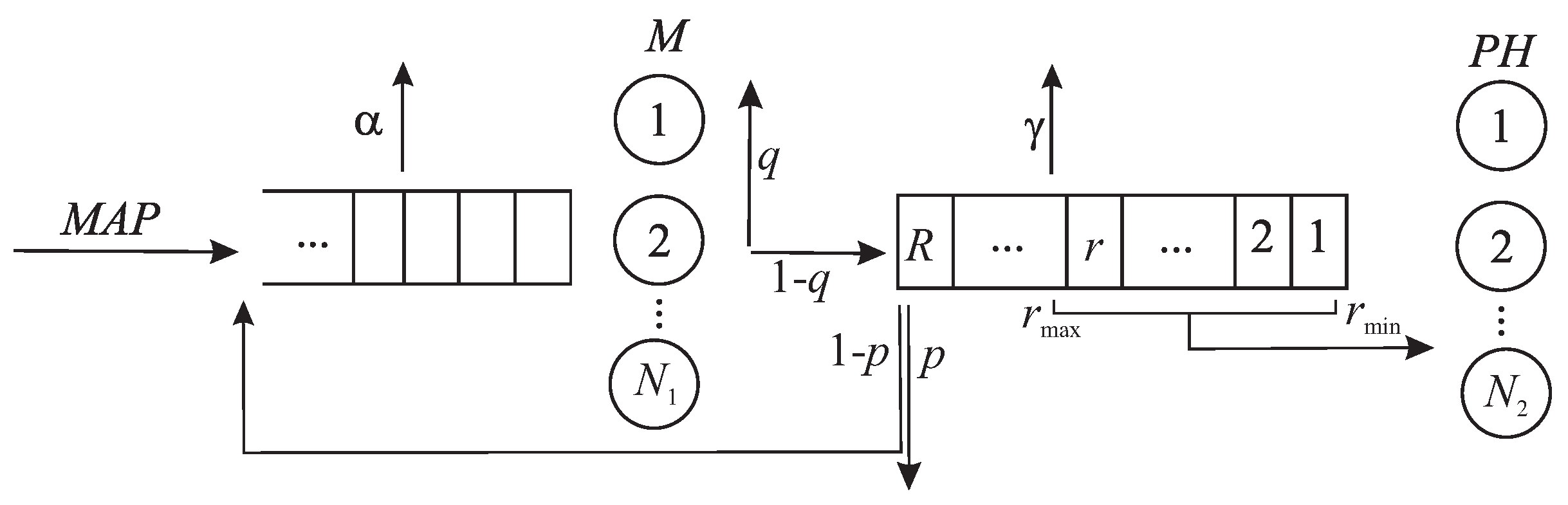
We consider a tandem queuing system consisting of two stages. The Stage 1 operation is described as a multi-server queuing system with independent, identical servers and an infinite buffer. The queuing system describing Stage 2 has independent identical servers and a finite buffer of capacity The scheme of the tandem operation is shown in Figure 1.
Customers enter the tandem system in the flow defined by the . This arrival process is given by an irreducible Markov chain with continuous time having a finite state space , and matrices and such that the matrix consists of the intensities of transitions of the chain , accompanied by the arrival of a customer. The non-diagonal elements of the matrix determine the intensity of the corresponding transition of the chain without the arrival of a customer, and the modules of the negative diagonal elements determine the intensity of the exit of the process from the corresponding state. The matrix is the generator of the Markov chain
The average customer rate is determined by the formula where is a row vector of stationary probabilities of the Markov chain This vector is the only solution to the system Here, and below, is a row vector of appropriate size consisting of zeros, and is a column vector of appropriate size consisting of ones.
More detailed information about the can be found, e.g., in [18,19,20,21,22]. The problem of construction of the for description of the traffic in a real-world system based on information about the traces of the flow was considered, e.g., in [23,24,25,26,27].
An arriving customer starts service at the Stage 1 if there is at least one idle server. Otherwise, it becomes buffered and waits for the release of one of the servers. At Stage 1, customers are serviced one at a time, and their service time has an exponential distribution with the parameter
After receiving service at Stage 1, the customer can decide to leave the system without service at Stage 2 with the probability q or with the complementary probability, it can continue processing in the tandem and move to Stage 2.
Customers at Stage 2 are served by groups. Each of the servers at Stage 2 can serve a group of customers consisting of at least customers and no more than customers. Thus, the parameters and determine the minimum and maximum size of the group that can be taken for service.
If at the time a customer arrives at Stage 2 there are customers in the buffer of Stage 2, then the incoming customer becomes buffered and awaits service, and it does not matter whether there are free servers at this stage. If, at a customer arrival moment at Stage 2, the number of customers in the buffer at this stage is and there is a free server, then the group of size is picked up for servicing. If all servers are busy, the customer joins the buffer if it is not full. If the buffer is full, the customer leaves the system with the probability p or, with the complementary probability, returns to the Stage 1 of tandem.
If at the moment of a server releasing at Stage 2 (the end of a group service time), there are customers in the buffer of Stage 2, then a group of customers of size is picked up for service.
We assume that the group service time at Stage 2 has a phase-type () distribution specified by a Markov chain with the state space of the transient states and a unique absorbing state . The irreducible representation of the distribution of service of a group consisting of r customers is given as Note that is a stochastic row vector of dimension and the square matrix S of dimension M is a subgenerator. The average service time for a group of customers of size r is defined as . Note that by assuming that the initial probability vector of service time depends on the size of the group, we take into account the dependence of the service process on the size of the group. More information about the distribution can be found, e.g., in [28,29,30,31].
Note that in the majority of papers dealing with group service, the authors assume that the service time of a group does not depend on the size of the group. This assumption is not very bad because, e.g., in the description of transportation systems, the time of the journey of a bus or aircraft between cities does not essentially depend on the number of traveling passengers. This assumption significantly simplifies the analysis of the model, and this is the main motivation for imposing this assumption.
In some other real-world systems, this assumption is not very realistic. For example, in modeling goods or food delivery systems, the service time of a group may consist of the time required to deliver the goods to the target distribution area in the city and the times for delivering the items to concrete recipients within this area. Thus, the total delivery time of a group depends on the size of the group. This is why we consider the given above description of the distribution of service of a group consisting of r customers. Note that in some communication systems, group service corresponds to the broadcasting of information. In that case, if the service time of an individual customer has a distribution, then the service time of a group is the maximum of individual service times, see, e.g., [32], and also has the distribution with parameters depending on the size of the group in the same manner as we assume here.
It is worth noting that sometimes the assumption that service time distribution is of type, but not its special case such as the exponential distribution, is imposed to fit not only the mean service time but the higher moments of distribution, the variance in particular. Here, the situation is different. We impose this assumption with specifically chosen irreducible representation to significantly reduce the dimensionality of the considered Markov chain. If we would try to assume that the service time of groups of different sizes has exponential distribution with a parameter depending on the group size and there is a wide range of possible sizes, the process describing the service of customers receiving service will have a very large size, irrespective of the description of this process, see [33].
It is suggested that customers staying in the buffers of the first and second stages may become impatient and leave the tandem system without service, independently of other customers, after a random time having an exponential distribution with the rate and correspondingly. Impatience (reneging from the system due to waiting too long) is the typical feature of customers in many real-world systems. Impatience is related to various psychological factors if the customers are humans: obsolescence of information, perishing of the products, expiration of the established by the service level agreement upper limit for service beginning, departure of the waiting mobile user from the cell, etc. Customer impatience can imply under-utilization of the service facility and the decrease in the possible revenue by the service provider. Therefore, consideration of queuing systems with impatient customers is popular in the existing literature. For the surveys, see, e.g., [34,35]. The account of the impatience phenomenon is very important in the context of systems with group service because waiting for accumulation in the buffer of the required minimal number of customers in the presence of idle servers may be psychologically uncomfortable for customers and motivate them to leave the system without receiving the service if the waiting seems to be too long.
Note that the model of operation of Stage 2 of the tandem is close to the model of an isolated queuing system considered in [36]. However, the use of that model for description of the marginal distribution of the states of Stage 2 of the tandem considered here is impossible due to two reasons: (i) the model considered in [36] assumes the as the descriptor of the arrival flow while, due to the infinite capacity of the buffer at Stage 1, the output flow from that stage is not defined by the (ii) due to the existence of the possibility of the customer’s return to Stage 1 (in case of the intermediate buffer overflow) there is a strong dependence between two stages and exact decomposition of the tandem queue to two isolated queues is not possible. Therefore, consideration of the random process describing the simultaneous transition of the states of two stages is mandatory.
Thus, the key features of the considered tandem queuing model, which define its generality and possible wide applicability, are as follows:
- •
- flow of customers that allows the adequate fitting of real-world flows;
- •
- Infinite buffer at Stage 1 of tandem and finite intermediate buffer;
- •
- Possibility of a group service of customers at Stage 2 with the fixed lower and upper size of the group;
- •
- Possibility of the dependence of a group service time on the size of the group;
- •
- distribution of service time of a group at Stage 2;
- •
- Possibility of customers reneging from the system during waiting time at both stages and after service completion at Stage 1;
- •
- Possibility of customer loss or return to Stage 1 in case of an intermediate buffer overflow.
Our aim is to implement an analysis of the stationary behavior of the described tandem queuing system.
3. The Process Describing the Dynamics of the System and Its Stationary Analysis
3.1. Definition of the Process
Let be the number of customers at Stage 1 of the tandem, including the customers receiving service and waiting in the buffer; is the number of customers in the buffer of Stage 2; is the number of busy servers at Stage 2; is the state of the underlying process of the is the number of servers on the k-th phase of service, at time
The behavior of the tandem system under study is described by a regular irreducible Markov chain with continuous time ()
The chosen way of describing simultaneous service processes in several parallel servers is traced back to [37,38] and is called the CSFP (count-server-for-phase) approach in [33]. Application of this approach leads to the necessity of more difficult analytical work compared to the TPFS (track-phase-for-server) approach. But its application allows us to significantly reduce the size of the blocks of the generator of describing the behavior of the system. In turn, this makes it feasible to implement the computation of the steady state distribution of for not only very small numbers of servers and capacity of the intermediate buffer.
3.2. Generator of the Process
Let us renumber the states of the in the direct lexicographical order of the components and reverse the lexicographical order of the components and call the set of states of the chain having the value i of the first component of the as level The set of states of the chain having the values of the first and second components of the is called the sub-level
To write down the expression for the infinitesimal generator of the we need the following denotations:
I is the identity matrix, and O is the zero matrix, the dimension of which is indicated by a subscript if necessary;
is the Kronecker delta, that is,
is the diagonal matrix with diagonal elements
is the square matrix with non-zero updiagonal elements
is the square matrix with non-zero subdiagonal elements
The numbers specify the cardinality of the state space of the vector process when n servers of Stage 2 are busy. They are calculated as
The matrix defines the transition intensities of the process at the moment when service in one of n busy servers at Stage 2 is completed,
The matrix contains the transition intensities of the process at the moment of the change in the phase of service in one of n busy servers of Stage 2,
The matrix defines the transition probabilities of the process at the moment when the group of r customers starts service in the presence of n busy servers of Stage 2,
The diagonal elements of the diagonal matrix determine the rates of the exit of the process from the corresponding states. The matrices are computed by the formula
The detailed description of the matrices , , and algorithms for their calculation are presented in [37,38,41].
The following statement is true.
Theorem 1.
The generator Q of the has the following block tridiagonal structure:
where the non-zero blocks containing the intensities of transitions from level i to level j are defined as follows.
- 1.
- The diagonal blocks have the form where the non-zero blocks are given as
- 2.
- The updiagonal blocks are the block diagonal matrices with the diagonal blocks of the form
- 3.
- The subdiagonal blocks have the form where the non-zero blocks are given as
Proof.
The theorem is proved by studying the intensities of all conceivable transitions of the during an infinitesimal time period.
Since during such a period customers enter the system and receive service at Stage 1 one at a time, the matrices are zero matrices for all such that
The blocks are built from the matrices containing the transition rates of the from the sub-level to the sub-level , .
Let us explain the form of all these blocks.
- The matrices have the following non-zero blocks:
- •
- the diagonal blocks
- •
- the subdiagonal blocks
- •
- updiagonal blocks
- •
- the blocks
- •
- the blocks
This is explained by the fact that during an interval of infinitesimal length, customers can arrive at the buffer of Stage 2 one-by-one, leave it one at a time due to impatience, and move to service in groups of size where- The diagonal elements of the diagonal blocks are negative. Their modules determine the intensity of departure of the from the respective state. The can exit from its current state in the following cases:
- (a)
- The underlying process of customer arrival leaves the current state. The corresponding transition intensities are determined up to sign by the diagonal entries of the matrix for and the matrix for
- (b)
- One of the busy servers’ service processes at Stage 2 changes its phase. In this case, the transition rates are determined by the diagonal entries of the matrix if and matrix if
- (c)
- A customer from the buffer of Stage 2 leaves this stage due to impatience. The corresponding rates are given by the matrices and
- (d)
- A customer from the buffer of Stage 1 leaves this stage due to impatience. The matrices if and if set the corresponding intensities.
- (e)
- A customer successfully finishes service at Stage 1. The corresponding intensities are set by the matrices if and if
- (f)
- A customer, after successful service at Stage 1 moves to Stage 2, finds the full buffer of Stage 2, and returns to Stage 1. The corresponding rates are given by the matrix .
- The non-diagonal entries of the matrices of the matrices determine the transition rates of the without changing the values of the components i and r. These transitions are defined by
- (a)
- The non-diagonal entries of the matrix if or if when the underlying process makes a jump without an customer generation;
- (b)
- The entries of the matrix when the process makes a transition implying the finish of the service, but a new service does not begin, since the number r of the customers in the buffer of Stage 2 is such that
- (c)
- The entries of the matrix if and matrix if when the process makes a jump that does not lead to service termination;
- The blocks contain the transition rates of the occurring when the number of customers in the buffer at Stage 2 decreases by one. This can happen only when a customer leaves this buffer due to impatience.Thus, the matrices are given by the matrix if the matrix for and the matrix if
- Let us explain in more detail the form of blocks when andIf , then a released server of Stage 2 always starts service if the buffer of this stage is not empty. The reduction in the number of customers in the buffer occurs if the service at Stage 2 is finished or a customer leaves the buffer due to impatience. The rates of occurring these events are specified by the matrices and , respectively.
- Next, let us comment on the expressions for the blocks specifying the transition rates of the process from the sub-level to the sub-level which occurs when r customers are accepted for simultaneous service at Stage 2. The corresponding rates are given by the entries of the matrixfor if and for if
- There is also a possible situation when, at the moment of realizing the server of Stage 2, there are customers in the buffer of Stage 2, then the group consisting of customers goes to service at Stage 2. The corresponding rates are given by the components of the matrixfor and by the components of the matrix ifAs a result of the presented considerations, we obtain the expressions for the blocks presented above.
- The updiagonal blocks contain the transition rates of the occurring when the number of customers at Stage 1 increases. This can only occur when a new customer enters the system. Therefore, these blocks are specified by the matrix if and by the matrix if .
- The subdiagonal blocks contain the rates of the transition when the number of customers at Stage 1 decreases by one. This can occur under the following scenarios:
- a customer at Stage 1 leaves the buffer due to impatience. In this case, blocks have the non-zero diagonal blocks which are specified by the matrix if and if
- a customer decides to leave the system after successful service at Stage 1. In this case, the transition rates are defined by the matrix for and by the matrix for
- a customer is lost after successful service at Stage 1, moving to Stage 2 and finding the full buffer of Stage 2. The intensities of this event occurrence are given by the entries of the matrix
- If besides cases and [], we also need to count the case when, after service at Stage 1, the customer decides to continue service at Stage 2, finds a free device, and immediately goes to service. That is why the block contains the additional summand
- The blocks also have a non-zero block given by the formula , which specifies the transition intensity of the in the case when a customer after service at Stage 1, moves to second stage and enters the buffer of this stage when it already contains customers and then a group of goes for service.
- The blocks also have the non-zero blocks which contain the rates of transitions from the sub-level to the sub-level An increase in the number of customers in the buffer of Stage 2 may occur when a customer, after service at Stage 1, attends Stage 2. The intensities of the corresponding transitions are specified by the matrix if by the matrixfor and by the matrix if
The theorem has been proven. □
3.3. Ergodicity of the Process
Having obtained the explicit form of the generator, it is possible to implement the analysis of the stationary distribution of the states of the system. The first part of such an analysis consists of the derivation of the condition for ergodicity of the This derivation differs in the cases when the impatience rate at Stage 1 is strictly positive and when it is equal to zero.
In the first case, looking at the explicit expressions for the blocks of the generator, it is not difficult to verify that the following limits exist:
where if and otherwise, and the matrix is the diagonal matrix whose diagonal entries coincide with the diagonal entries of the matrix taken with the opposite sign.
Existence of the limits (1) implies, according to the definition given in [42], that the is the particular case of the asymptotically quasi-Toeplitz Markov chains ().
Sufficient condition for ergodicity of obtained in [42] in the case when the matrix is irreducible is the fulfillment of inequality
where the row vector is the unique solution of the system
Calculating the explicit expressions for matrices from (1), we can easily verify that Thus, the inequality (2) is trivially fulfilled. Therefore, if the impatience rate at Stage 1 is strictly positive then the is ergodic for any set of the system parameters.
In the second case, when the is the level-independent quasi-birth-and-death process with many boundary levels (level independence takes place for levels i such that ) the criterion of ergodicity for the is obtained immediately from the results by M. Neuts, see [28], as follows.
Let be equal to the matrix if is set to be equal 0.
Let and
According to [28], the is ergodic if and only if the inequality
is fulfilled where the row vector is the unique solution to equations
Thus, to verify whether or not the is ergodic it is necessary to solve the finite system (4) of the linear algebraic equations and verify whether or not the inequality (3) holds good.
If the return of a customer to Stage 1 due to the overflow of the buffer at Stage 2 is impossible (), the criterion of ergodicity is reduced to the requirement of fulfillment of inequality
3.4. Outline of Calculation of Stationary Distribution of the Process
Let the considered be ergodic. Then the following stationary probabilities of the states exist:
Let us form the row vectors of the stationary probabilities of the states belonging to the sub-level and the vectors of the stationary probabilities of the states belonging to the level
It is well known that the row vectors satisfy the system of equations:
In the case when the customers at Station 1 are absolutely patient (), the vectors can be found in so-called matrix-geometric form, see [28].
4. Formulas for Computation of the Values of the Key Performance Measures of the System
The goal of the computation of the stationary distribution of the states of any queuing model is its use for the computation and optimization of the main performance indicators of the system. Let us present some formulas for their computation.
The average number of customers in the buffer of Stage 1 is calculated using the formula
The average number of busy servers at Stage 1 is calculated using the formula
The average number of customers at Stage 1 is calculated using the formula
The average number of customers in the buffer of Stage 2 is calculated using the formula
The average number of busy servers in Stage 2 is calculated by the formula
The average number of customers at Stage 2 is calculated using the formula
where the vectors are defined by the partition
The average intensity of the output flow of successfully serviced customers from Stage 1 is calculated by the formula
The average intensity of the output flow of successfully serviced customers from Stage 2 is calculated by the formula
The average intensity of the input flow of customers to Stage 2 is calculated by the formula
The average intensity of the input flow of customers to Stage 2 that were accepted for this stage is calculated by the formula
The probability that an arriving customer will find an idle server at Stage 1 and enter the service is found by the formula
The probability that an arriving customer will find all busy servers at Stage 1 and go to the buffer is found by the formula
The rate of customer leaving the buffer of Stage 2 for service is calculated by the formula
The probability that a customer, after service at Stage 1, will find the buffer of Stage 2 full and leave the system is found by the formula
The probability that a customer, after service at Stage 1, attends Stage 2 is found by the formula
The loss probability of an arbitrary customer from the buffer of Stage 1 due to impatience is calculated using the formula
The loss probability of an arbitrary customer from the buffer of Stage 2 due to impatience is calculated using the formula
The loss probability of a customer being accepted to Stage 2 from the buffer of Stage 2 due to impatience is calculated using the formula
The average size of the group that is picked up for service at Stage 2 is calculated as
The loss probability of an arbitrary customer in Stage 1 is calculated using the formula
The loss probability of an arbitrary customer in Stage 2 is calculated using the formula
The loss probability of an arbitrary customer is calculated using the formula
Remark 1.
The algorithm for computation of the stationary probability vectors, which we used for computation of different performance measures of the system in the following section, is numerically stable, but expressions for the blocks of the generator are quite bulky. Therefore, computer realization of the algorithm is not easy and its control is mandatory. Beside various other means for control, Formula (5) giving two different possibilities for the loss probability calculation can be used for the accuracy of realization and computation control.
5. Numerical Example
The considered tandem system has a lot of parameters, each of which has an impact on performance metrics of the system that deserves a detailed illustration. For example, this concerns the mean arrival rate, the coefficients of variation and correlation of inter-arrival times, number of servers at both stages of tandem, service rate at Stage 1, capacity of the intermediate buffer, impatience rates of customers at both buffers, probabilities of abandonment of service at Stage 2 and customer return to Stage 1 in case of the intermediate buffer overflow. However, because the main novelty of the model consists of the possibility of group service at Stage 2 with restriction on the minimum and maximum of a group size and dependence of service time on the size of a serviced group, we state as the goal of this example to highlight the impact of the thresholds and defining the borders of a size of a group that can be serviced at Stage 2 of the tandem and illustrate the possibility of the optimal choice of these thresholds. We present the results illustrating this impact under the fixed below set of the other system parameters.
Let the number of servers at Stage 1 be , the number of servers at Stage 2 be and the capacity of the buffer at Stage 2 be
Customers enter the tandem system in the flow defined by the matrices
This flow has the average customer rate the coefficient of correlation of successive inter-arrival times and the coefficient of variation of these times .
The service rate of the customer at Stage 1
We assume that the mean service time of a group consisting of r customers, at Stage 2 is defined by formulas
Such a choice of parameters implies that the average service time of the first customer in the group is 25 min; each subsequent customer in the group adds 6 min to the average service time of the group. To obtain these values of the mean service times, we choose a phase-type distribution with the irreducible representation , where
The mean service time of the groups monotonously increases, with the increase in the number of customers in a serviced group from 1 to 30, from 25 to 199. The coefficient of variation of the group service time varies as follows. For the group size equal to 1, the vector is given by This implies that service time of a group consisting of one customer has the exponential distribution with the rate Correspondingly, the coefficient of variation of such a group service time is equal to one. With growth of group size r, service time distribution becomes hyper-exponential distribution that has the coefficient of variation greater than one. This coefficient increases with the growth of group size For the values of this coefficient are 3.09781, 3.84003, 4.03732, respectively. However, then this coefficient starts decreasing. For , it takes values 3.99875, 3.8562, 3.07659, 1.70804, and 1.05412, 1, correspondingly. The initial growth of the coefficient of variation of the group service time with its further decrease fits the behavior of the service time interpreted as parcels delivering from the warehouse to some district of the city. The main amount of time is spent on the car trip from the warehouse to the district. Delivering of parcels to each client inside the district adds smaller amount of time to the total time during which the car will be busy by delivering. Initial increase in the variance of the delivering time is caused by the raise in uncertainty of the total delivering time due to the adding of complimentary random times of delivering to an individual client. The variance starts decreasing with the further growth of the number of delivered parcels due to the law of large numbers. Value 1 of the coefficient of variation when is easily explained by the fact that the vector is given by what implies that service time of a group consisting of R customers has the exponential distribution with the rate
The impatience rates at Stages 1 and 2 are and , respectively. The probabilities p and q are chosen as and .
Let us vary the parameter in the range from 1 to 30 and the parameter in the range from to R with Step 1.
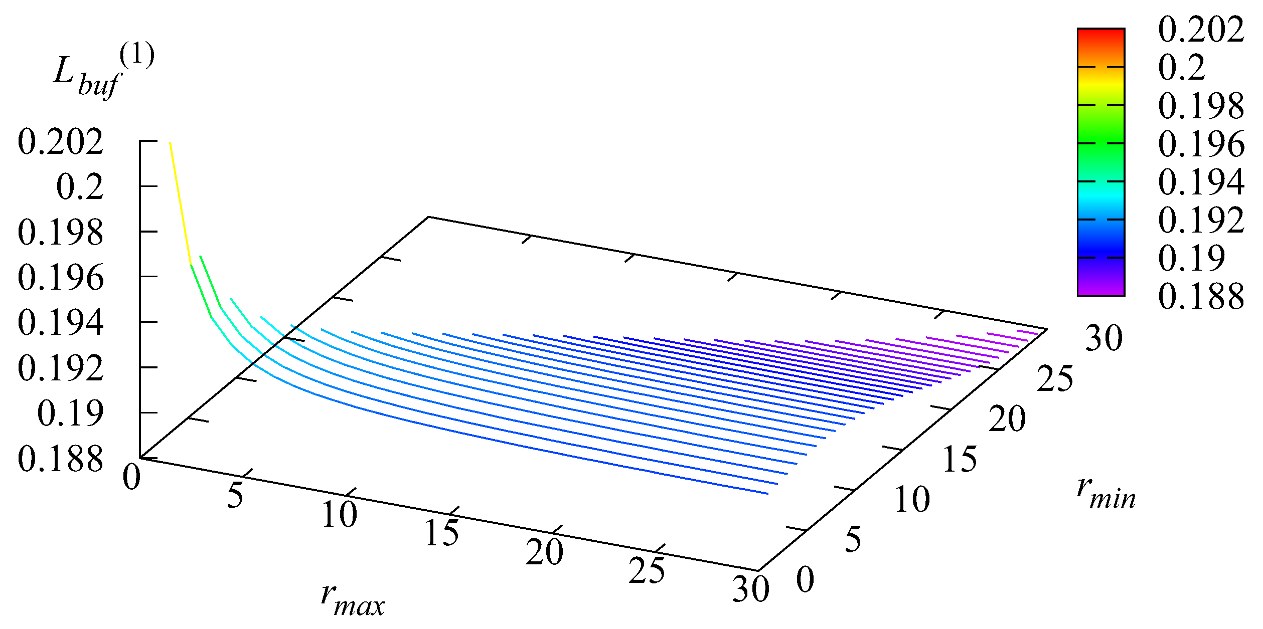
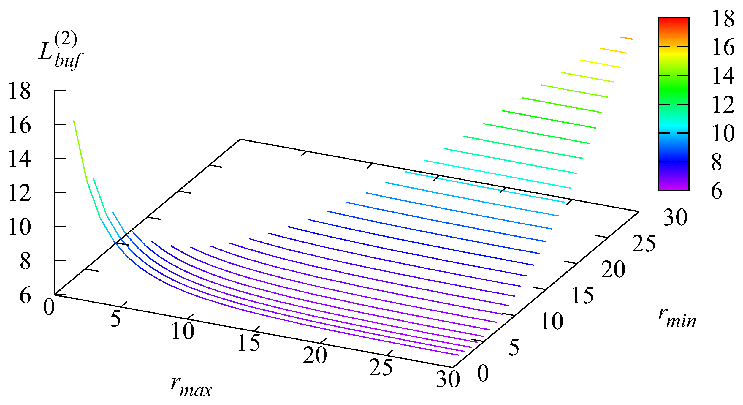
Figure 2 and Figure 3 illustrate the dependencies of the average number of customers in the buffer of Stage 1, and Stage 2, under different values of the parameters and
The form of the shape presented in Figure 3 is explained as follows. The service of customers in the larger groups is profitable in terms of the average service time per customer. For the group consisting of r customers, the latter time is defined as
and evidently decreases when r increases. When the numbers and are small, this advantage of group service is weakly used. When increases, this advantage starts working and decreases. However, with the subsequent growth of the number starts to increase because the large values of lead to the accumulation of the larger number of customers in the second buffer until service beginning. This leads to the starvation of servers at Stage 2, their under-utilization, and, finally, the increase in the average number of
The form of the shape presented in Figure 2 correlates with Figure 3. When the numbers and are small, the mentioned advantage of group service is not used. This implies a high probability that the buffer of Stage 2 is full and the customer who finished service at Stage 1 returns (with the probability ) for service at Stage 1. When increases, this advantage starts to work, and the probability of the second buffer overflow decreases. Correspondingly, the rate of customer’s return to Stage 1 decreases, which causes the decrease of However, with the subsequent growth of the number starts to increase (because, as noted above, the large values of lead to the accumulation of a larger number of customers in the second buffer). Simultaneously, the probability of the second buffer overflow becomes higher. The essential increase in the value of when and become large, which is observed in Figure 2, does not induce the growth of because many customers renege from the second buffer due to impatience but do not return to Stage 1.
It is worth noting that it is hardly possible to give more exact intuitive explanation of the shape of surfaces presented in Figure 2 and Figure 3 due to the complexity of the model. In particular, the difficulty of explanations is related with the fact that variation of the thresholds and causes the change of the distribution of the size of the serviced groups while, as it was noted above, variance of the service time non-monotonically behaves when the size of a group varies. It is well known that the average queue length depends on the variance of the service time. Thus, the complicated non-monotonic behavior of this variance makes the intuitive explanation difficult. This makes valuable algorithmic and numerical analysis of the considered tandem.
Figure 4 shows the dependence of the average number of busy servers at Stage 2 on the parameters and
This number achieves its maximum when is small, the advantages of group service are not exploited, and, therefore, more servers of Stage 2 must work. When increases, servers are used more effectively, and the average number of busy servers at Stage 2 decreases. The influence of the threshold in this example is not very significant.
Figure 5 shows the dependence of the average size of the group, which is picked up for service at Stage 2, on the parameters and As can be expected, the number is minimal when the restriction on the minimum size of a group is weak. essentially increases when this restriction becomes stronger. Finally, when all customers are served in groups of size 30. The dependence of on is not so essential. obviously increases when becomes larger. But for large values of the increase becomes slow due to the fact that the number of used servers also depends on the arrival rate. For the fixed arrival rate, the number of used servers (and the average size of the group) are restricted from above.
Therefore, dependence of can be summarized as follows. For all values of , monotonically increases when grows from to The range of values of monotonically decreases when grows. For example, for the value of grows from 1 to 5.26 (the difference is 4.26). For the value of varies from 2 to 5.59 (the difference is 3.59). For the value of varies from 8 to 9.66 (the difference is 1.66). For the difference is 0.21. For the difference is 0.006. Note that these dependencies are qualitatively clear. But the worth of our numerical results is in giving the exact quantitative characterization of these probabilities.
Figure 6, Figure 7, Figure 8, Figure 9 and Figure 10 show the dependencies on the parameters and of the loss probabilities of an arbitrary customer due to various reasons. and are the probabilities of the loss from Stages 1 and 2. The loss at Stage 1 is caused by the impatience of customers in the first buffer. As it is clear from the formula for its computation, the loss probability is proportional to the average number of customers in the buffer of Stage 1. Figure 2 and Figure 6 confirm this. The loss at Stage 2 may occur due to the impatience of customers from the buffer and due to the second buffer overflow. is the probability of a loss due to the buffer overflow. is the probability of the loss from the buffer of Stage 2 due to impatience. Because, in this example, the probability is quite small, the shape of the surface presented in Figure 7 is very similar to the shape of the surface presented in Figure 9. The probability presented in Figure 10 is the probability of the loss of a customer accepted to Stage 2 due to impatience. It is slightly larger than the probability presented in Figure 10 because the value of the arrival rate to the system in the denominator of the formula for computation of is greater than the value of the arrival rate of admitted to Stage 2 customers in the denominator of the formula for computation of
As it is evident from Figure 2, Figure 3, Figure 4, Figure 5, Figure 6, Figure 7, Figure 8, Figure 9 and Figure 10, the performance measures of the system admit values in a wide range when the thresholds and vary. Therefore, it is reasonable to use the results of computation of these measures for optimization of the operation of the system. Various optimization problems can be formulated and solved.
For example, the quality of the system’s operation can be evaluated in terms of the following cost criterion:
Here, a and b are the revenue of the system earned via the service of one customer at Stages 1 and 2, correspondingly; c and d are the charges for the loss of an arbitrary customer at Stages 1 and 2; and f is the cost for maintaining one place in a service device (a delivery vehicle) per unit of time. This criterion E determines the average profit obtained by the system per unit of time, and our managerial goal is to obtain such parameters as and under which the system’s revenue is maximal.
In this numerical example, let us set the following values for the cost coefficients:
Figure 11 shows the dependence of the cost criterion E on the parameters and
The optimal value of the cost criterion is equal to 0.340837. It is achieved under the following values of the thresholds: When all customers are serviced at Station 2 one-by-one, i.e., , and the advantages of group service are not used, the value E is −1.4909. Let us leave which means that all servers at Stage 2 are busy when the buffer is non-empty, and increase we more fully use the advantages of group service. The value of E increases up to the value achieved for The cost criterion achieves the value 0.32. The further increase of from 18 to 30 leads the monotonic decrease of E to the value of 0.2852.
When we start the increase of , the value of E increases. For , the value of E becomes positive. The optimal value of the cost criterion is equal to 0.340837. It is achieved under the following values of the thresholds: When we further increase the values of , the value of the cost criterion becomes worse, even for the best choice of For the value of E becomes negative for any . This means that the use of the advantage of group service increases. But simultaneously, it increases the charge for maintaining the capacity of the service devices. For the value of the cost criterion is −1.2471.
Thus, this example highlights the possibility of essentially improving the effectiveness of the system operation via the proper use of the minimal and maximal sizes and of the groups picked up from the buffer for service.
If we modify the optimization problem by imposing an additional constraint on the average number of the average size of the group that is picked up for service at Stage 2. Such a constraint is reasonable, e.g., if each customer (passenger) books a ticket and the system manager would like to have a definite average profit from each service (calculated as the difference between the money paid by the passengers and expenditures of the service provider, including payment of a vehicle lease, fuel, taxes, the service team’s or driver’s salary, etc.). Under such an additional constraint, the optimal values and become equal to 6 and 22, respectively. The optimal revenue becomes equal to 0.3147.
6. Conclusions
In this paper, we considered the novel two-stage tandem queuing system. Customer arrival process may have the fluctuating instantaneous rate, correlation of the subsequent inter-arrival times and versatile values of their variance. This process considerably more adequately describes the flows in real-world systems than the stationary Poisson process supposed in the majority of the existing research of the tandem queuing systems. The most distinctive feature of the considered model is the possibility of group service for customers at Stage 2 and dependence of the group service time on the size of a group. The distribution of the service time of a group of any fixed size has a distribution with irreducible representation depending on the size of the group.
Both stages of the tandem are described by the multi-server systems with impatient customers that may renege from the tandem without receiving service if their waiting time reaches the fixed in advance value having an exponential distribution. While the analysis of the tandem is presented here for both cases, with absolutely patient and impatient customers, account of the possible impatience increases the adequacy of the considered model to real-world systems. The possibility that customers received service at Stage 1 depart from the tandem without trying to receive service at Stage 2 is suggested. Such a departure can occur, e.g., in the following two cases: the customer has received all required service at Stage 1 and does not need service at Stage 2; preliminary service of the customer at Stage 1 was not satisfactory and he/she decides to skip the main service at Stage 2. The possibility of customers, which have received service at Stage 1, losing or returning to Stage 1 due to a finite intermediate buffer overflow is also suggested.
The behavior of the system is described by the including the number of customers at Stage 1 of the tandem, the number of customers in the buffer of Stage 2, the number of busy servers at Stage 2, the state of the underlying process of the and the number of servers at each phase of service at Stage 2. This is the well-studied level-independent quasi-birth-and-death process in case of the patient customers and the in case of the impatient customers. Stationary analysis of this under the fixed values (thresholds) of the minimum and maximum size of the groups, service to which is provide at Stage 2, is implemented. The significant impact of these values on the main performance indicators of the tandem is numerically highlighted. An example of solving the problem of the service provider’s revenue maximization is presented. This example confirms the possibility of essentially improving the effectiveness of the system operation via the proper use of the thresholds.
The considered model can be applied to designing and managing various telecommunication, logistic, production, manufacturing, and other systems and networks in which service can be decomposed into two stages, e.g., the preliminary (auxiliary) service and the main (essential) service. For example, in modeling of very popular now systems of a food or goods delivering, Stage 1 corresponds to the acceptance of an order from a customer and packing the required items to some container for delivering. Stage 2 corresponds to the container delivering to the customer by some transport. Simultaneous delivering of the container to many customers is very common to reduce the provider expenditures related to the use of the transport. The obtained results can be used for the choice of suitable capacity of two service devices and their optimal matching as well as for optimization of the thresholds defining the minimum and maximum size of the groups to which service can be provided. These sizes can predefine the capacity of the required transport units and economically feasible restrictions on the minimal number of delivered orders.
Results of the presented analysis can be used for the study of various extensions of the considered model. For example, customers arriving at Stage 1 when all servers are busy cannot be buffered but should retry for service later on. Customers are heterogeneous and some of them have a priority in access to service at one or both stages. Servers can be completely or partially unreliable. There is a cross-traffic of customers arriving directly to Stage 2. Parameters of the system are influenced by an external random process, etc.
Author Contributions
Conceptualization, S.A.D. and O.S.D.; methodology, S.A.D., A.N.D. and O.S.D.; software, S.A.D. and O.S.D.; validation, S.A.D. and O.S.D.; formal analysis, S.A.D. and O.S.D.; investigation, S.A.D., A.N.D. and O.S.D.; writing, original draft preparation, S.A.D., A.N.D. and O.S.D.; writing, review and editing, S.A.D., A.N.D. and O.S.D.; supervision, S.A.D.; project administration, O.S.D. All authors have read and agreed to the published version of the manuscript.
Funding
This research received no external funding.
Data Availability Statement
Data are contained within the article.
Conflicts of Interest
The authors declare no conflicts of interest.
References
- Neuts, M.F. Two queues in series with a finite, intermediate waiting room. J. Appl. Probab. 1968, 5, 123–142. [Google Scholar] [CrossRef]
- Gnedenko, B.W.; Konig, D. Handbuch der Bedienungstheorie; Akademie Verlag: Berlin, Germany, 1983. [Google Scholar]
- Balsamo, S.; Persone, V.D.N.; Inverardi, P. A review on queuing network models with finite capacity queues for software architectures performance prediction. Perform. Eval. 2003, 51, 269–288. [Google Scholar] [CrossRef]
- Perros, H.G. A bibliography of papers on queuing networks with finite capacity queues. Perform. Eval. 1989, 10, 255–260. [Google Scholar] [CrossRef]
- Balsamo, S. Queueing networks with blocking: Analysis, solution algorithms and properties. In Network Performance Engineering: A Handbook on Convergent Multi-Service Networks and Next Generation Internet; Springer: Berlin/Heidelberg, Germany, 2011; pp. 233–257. [Google Scholar]
- Baumann, H.; Sandmann, W. Multi-server tandem queue with Markovian arrival process, phase-type service times, and finite buffers. Eur. J. Oper. Res. 2017, 256, 187–195. [Google Scholar] [CrossRef]
- Dudin, S.A.; Dudin, A.N.; Dudina, O.S.; Chakravarthy, S.R. Analysis of a tandem queuing system with blocking and group service in the second node. Int. J. Syst. Sci. Oper. Logist. 2023, 10, 1–20. [Google Scholar] [CrossRef]
- Chakravarthy, S.R. Analysis of a finite MAP/G/1 queue with group services. Queuing Syst. Theory Appl. 1993, 13, 385–407. [Google Scholar] [CrossRef]
- Chakravarthy, S.R.; Shruti, G.; Rumyantsev, A. Analysis of a queuing model with batch markovian arrival process and general distribution for group clearance. Methodol. Comput. Appl. Probab. 2021, 23, 1551–1579. [Google Scholar] [CrossRef]
- Chakravarthy, S.; Alfa, A.S. A multiserver queue with Markovian arrivals and group services with thresholds. Nav. Res. Logist. (NRL) 1993, 40, 811–827. [Google Scholar] [CrossRef]
- Chakravarthy, S.R. Analysis of a multi-server queue with batch Markovian arrivals and group services. Eng. Simul. 2000, 18, 51–66. [Google Scholar]
- Chakravarthy, S.; Alfa, A.S. A finite capacity queue with Markovian arrivals and two servers with group services. J. Appl. Math. Stoch. Anal. 1994, 7, 161–178. [Google Scholar] [CrossRef]
- Chakravarthy, S.R. A Finite Capacity GI/PH/1 Queue with Group Services. Nav. Res. Logist. 1992, 39, 345–357. [Google Scholar] [CrossRef]
- Banik, A.D. Queueing analysis and optimal control of BMAP/G(a,b)/1/N and BMAP/MSP(a,b)/1/N systems. Comput. Ind. Eng. 2009, 57, 748–761. [Google Scholar] [CrossRef]
- Claeys, D.; Steyaert, B.; Walraevens, J.; Laevens, K.; Bruneel, H. Analysis of a versatile batch-service queuing model with correlation in the arrival process. Perform. Eval. 2013, 70, 300–316. [Google Scholar] [CrossRef]
- Ghosh, S.; Banik, A.D.; Walraevesn, J.; Bruneel, H. A detailed note on the finite-buffer queuing system with correlated batch-arrivals and batch-size phase-dependent bulk-service. 4OR-Q J. Oper. Res. 2022, 20, 241–272. [Google Scholar] [CrossRef]
- Nikoui, T.S.; Rahmani, A.M.; Balador, A.; Javadi, H.H.S. Analytical model for task offloading in a fog computing system with batch-size-dependent service. Comput. Commun. 2022, 190, 201–215. [Google Scholar] [CrossRef]
- Chakravarthy, S.R. The batch Markovian arrival process: A review and future work. Adv. Probab. Theory Stoch. Process. 2001, 1, 21–49. [Google Scholar]
- Chakravarthy, S.R. Introduction to Matrix-Analytic Methods in Queues 1: Analytical and Simulation Approach-Basics; ISTE Ltd.: London, UK; John Wiley and Sons: New York, NY, USA, 2022. [Google Scholar]
- Dudin, A.N.; Klimenok, V.I.; Vishnevsky, V.M. The Theory of Queuing Systems with Correlated Flows; Springer Nature: Cham, Switzerland, 2020. [Google Scholar]
- Lucantoni, D. New results on the single server queue with a batch Markovian arrival process. Commun.-Stat.-Stoch. Model. 1991, 7, 1–46. [Google Scholar] [CrossRef]
- Lucantoni, D.M. “The BMAP/G/1 queue: A tutorial”. Performance Evaluation of Computer and Communication Systems. Lecture Notes Comput. Sci. 1993, 729, 330–358. [Google Scholar]
- Buchholz, P.; Kriege, J. A heuristic approach for fitting MAPs to moments and joint moments. In Proceedings of the Sixth International Conference on the Quantitative Evaluation of Systems, Budapest, Hungary, 13–16 September 2009; pp. 53–62. [Google Scholar]
- Buchholz, P.; Kemper, P.; Kriege, J. Multi-class Markovian arrival processes and their parameter fitting. Perform. Eval. 2010, 67, 1092–1106. [Google Scholar] [CrossRef]
- Buchholz, P.; Panchenko, A. Two-Step EM Algorithm for MAP Fitting. Lecture Notes Comput. Sci. 2004, 3280, 217–272. [Google Scholar]
- Buchholz, P.; Kriege, J.; Felko, I. Input Modeling with Phase-Type Distributions and Markov Models Theory and Applications; Springer: Berlin/Heidelberg, Germany, 2014. [Google Scholar]
- Casale, G. Building accurate workload models using Markovian arrival processes. ACM Sigmetrics Perform. Eval. Rev. 2011, 3, 357–358. [Google Scholar]
- Neuts, M. Matrix-Geometric Solutions in Stochastic Models; The Johns Hopkins University Press: Baltimore, MD, USA, 1981. [Google Scholar]
- Asmussen, S. Applied Probability and Queues; Springer: New York, NY, USA, 2003; Volume 2. [Google Scholar]
- O’Cinneide, C.A. Characterization of phase-type distributions. Stoch. Model. 1990, 6, 1–57. [Google Scholar] [CrossRef]
- O’Cinneide, C.A. Phase-type distribution: Open problems and a few properties. Commun. Stat. Stoch. Model. 1999, 15, 731–757. [Google Scholar] [CrossRef]
- Dudin, A.N.; Manzo, R.; Piscopo, R. Single server retrial queue with group admission of customers. Comput. Oper. Res. 2015, 61, 89–99. [Google Scholar] [CrossRef]
- He, Q.M.; Alfa, A.S. Space reduction for a class of multidimensional Markov chains: A summary and some applications. INFORMS J. Comput. 2018, 30, 1–10. [Google Scholar] [CrossRef]
- Sharma, S.; Kumar, R.; Soodan, B.S.; Singh, P. Queuing models with customers’ impatience: A survey. Int. J. Math. Oper. Res. 2023, 26, 523–547. [Google Scholar] [CrossRef]
- Stanford, R.E. On queues with impatience. Adv. Appl. Probab. 1990, 22, 768–769. [Google Scholar] [CrossRef]
- Dudin, S.; Dudina, O. Analysis of a multi-server queue with group service and service time dependent on the size of a group as a model of a delivery system. Mathematics 2023, 11, 4587. [Google Scholar] [CrossRef]
- Ramaswami, V. Independent Markov processes in parallel. Comm. Statist.-Stochastic Models 1985, 1, 419–432. [Google Scholar] [CrossRef]
- Ramaswami, V.; Lucantoni, D.M. Algorithms for the multi-server queue with phase type service. Stoch. Model. 1985, 1, 393–417. [Google Scholar] [CrossRef]
- Graham, A. Kronecker Products and Matrix Calculus with Applications; Courier Dover Publications: Garden City, NY, USA, 2018. [Google Scholar]
- Horn, R.A.; Johnson, C.R. Topics in Matrix Analysis; Cambridge University Press: Cambridge, UK, 1991. [Google Scholar]
- Kim, C.; Dudin, A.; Dudin, S.; Dudina, O. Mathematical model of operation of a cell of a mobile communication network with adaptive modulation schemes and handover of mobile users. IEEE Access 2021, 9, 106933–106946. [Google Scholar] [CrossRef]
- Klimenok, V.I.; Dudin, A.N. Multi-dimensional asymptotically quasi-Toeplitz Markov chains and their application in queuing theory. Queueing Syst. 2006, 54, 245–259. [Google Scholar] [CrossRef]
- Dudin, S.; Dudina, O. Retrial multi-server queuing system with PHF service time distribution as a model of a channel with unreliable transmission of information. Appl. Math. Model. 2019, 65, 676–695. [Google Scholar] [CrossRef]
- Dudin, S.; Dudin, A.; Kostyukova, O.; Dudina, O. Effective algorithm for computation of the stationary distribution of multi-dimensional level-dependent Markov chains with upper block-Hessenberg structure of the generator. J. Comput. Appl. Math. 2020, 366, 112425. [Google Scholar] [CrossRef]
Figure 1.
The structure of the tandem queue.

Figure 2.
The dependence of the average number of customers in the buffer of Stage 1 on the parameters and .
Figure 2.
The dependence of the average number of customers in the buffer of Stage 1 on the parameters and .

Figure 3.
The dependence of the average number of customers in the buffer of Stage 2 on the parameters and .
Figure 3.
The dependence of the average number of customers in the buffer of Stage 2 on the parameters and .

Figure 4.
The dependence of the average number of busy servers at Stage 2 on the parameters and .

Figure 5.
The dependence of the average size of the group that is picked up for service at Stage 2 on the parameters and .
Figure 5.
The dependence of the average size of the group that is picked up for service at Stage 2 on the parameters and .

Figure 6.
The dependence of the loss probability of an arbitrary customer from Stage 1 on the parameters and .
Figure 6.
The dependence of the loss probability of an arbitrary customer from Stage 1 on the parameters and .

Figure 7.
The dependence of the loss probability of an arbitrary customer from Stage 2 on the parameters and .
Figure 7.
The dependence of the loss probability of an arbitrary customer from Stage 2 on the parameters and .

Figure 8.
The dependence of the probability that a customer after service at Stage 1 will find the buffer of Stage 2 full and leave the system on the parameters and .
Figure 8.
The dependence of the probability that a customer after service at Stage 1 will find the buffer of Stage 2 full and leave the system on the parameters and .

Figure 9.
The dependence of the loss probability of an arbitrary customer from the buffer of Stage 2 due to impatience on the parameters and .
Figure 9.
The dependence of the loss probability of an arbitrary customer from the buffer of Stage 2 due to impatience on the parameters and .

Figure 10.
The dependence of the loss probability of an customer accepted to Stage 2 from the buffer of Stage 2 due to impatience on the parameters and .
Figure 10.
The dependence of the loss probability of an customer accepted to Stage 2 from the buffer of Stage 2 due to impatience on the parameters and .

Figure 11.
The dependence of the cost criterion on the parameters and .

Disclaimer/Publisher’s Note: The statements, opinions and data contained in all publications are solely those of the individual author(s) and contributor(s) and not of MDPI and/or the editor(s). MDPI and/or the editor(s) disclaim responsibility for any injury to people or property resulting from any ideas, methods, instructions or products referred to in the content. |
© 2024 by the authors. Licensee MDPI, Basel, Switzerland. This article is an open access article distributed under the terms and conditions of the Creative Commons Attribution (CC BY) license (https://creativecommons.org/licenses/by/4.0/).
Share and Cite
MDPI and ACS Style
Dudin, S.A.; Dudina, O.S.; Dudin, A.N. Analysis of Tandem Queue with Multi-Server Stages and Group Service at the Second Stage. Axioms 2024, 13, 214. https://doi.org/10.3390/axioms13040214
AMA Style
Dudin SA, Dudina OS, Dudin AN. Analysis of Tandem Queue with Multi-Server Stages and Group Service at the Second Stage. Axioms. 2024; 13(4):214. https://doi.org/10.3390/axioms13040214
Chicago/Turabian StyleDudin, Sergei A., Olga S. Dudina, and Alexander N. Dudin. 2024. "Analysis of Tandem Queue with Multi-Server Stages and Group Service at the Second Stage" Axioms 13, no. 4: 214. https://doi.org/10.3390/axioms13040214
Note that from the first issue of 2016, this journal uses article numbers instead of page numbers. See further details here.