
Probabilistic Assessment of Structural Integrity


1
Lithuanian Energy Institute, Breslaujos Str. 3, LT-44403 Kaunas, Lithuania
2
Department of Applied Mathematics, Kaunas University of Technology, Studentų Str. 50, LT-51368 Kaunas, Lithuania
*
Author to whom correspondence should be addressed.
Axioms 2024, 13(3), 154; https://doi.org/10.3390/axioms13030154
Submission received: 11 December 2023
/
Revised: 4 February 2024
/
Accepted: 16 February 2024
/
Published: 27 February 2024
(This article belongs to the Special Issue Methods and Applications of Advanced Statistical Analysis)
Abstract
:A probability-based approach, combining deterministic and probabilistic methods, was developed for analyzing building and component failures, which are especially crucial for complex structures like nuclear power plants. This method links finite element and probabilistic software to assess structural integrity under static and dynamic loads. This study uses NEPTUNE software, which is validated, for a deterministic transient analysis and ProFES software for probabilistic models. In a case study, deterministic analyses with varied random variables were transferred to ProFES for probabilistic analyses of piping failure and wall damage. A Monte Carlo Simulation, First-Order Reliability Method, and combined methods were employed for probabilistic analyses under severe transient loading, focusing on a postulated accident at the Ignalina Nuclear Power Plant. The study considered uncertainties in material properties, component geometry, and loads. The results showed the Monte Carlo Simulation method to be conservative for high failure probabilities but less so for low probabilities. The Response Surface/Monte Carlo Simulation method explored the impact load–failure probability relationship. Given the uncertainties in material properties and loads in complex structures, a deterministic analysis alone is insufficient. Probabilistic analysis is imperative for extreme loading events and credible structural safety evaluations.
Keywords:
probabilistic finite element analysis; structural integrity; sensitivity analysis; Monte Carlo Simulation; First-Order Reliability Method; Response Surface methodMSC:
82-XX; 82Mxx; 60H30; 62P301. Introduction
In the evaluation of complex and dynamic structures posing environmental risks, it is crucial to optimize and integrate strength analysis methods. However, relying on simulation-based optimization often produces a deterministic optimum design that pushes the limits of design constraints, offering little room for tolerances in modeling, uncertain simulations, and manufacturing imperfections. Consequently, obtaining deterministic optimum designs without considering uncertainty may lead to unreliable outcomes, necessitating the adoption of Reliability-Based Design Optimization [1].
For a structural integrity analysis of critical structures facing extreme internal or external loading events, the careful selection of numerical simulation methods, meticulous model preparation, and the evaluation of material properties and loads are paramount. While recognizing the uncertainty in every material parameter, it becomes especially important to assess uncertainties related to loads, material properties, geometrical parameters, boundaries, and other factors to ensure structures remain reliable and safe during accidental transient loading. Therefore, accounting for the uncertainty in these quantities is necessary when conducting a structural integrity evaluation [2]. This is achieved through probabilistic analyses, examining whether combinations of relevant parameters could lead to failure and determining the probability of failure [3,4].
This paper outlines the methodology of a probability-based structural integrity analysis, extending and integrating deterministic (validated) and probabilistic methods using state-of-the-art software.
The finite element method is employed for the deterministic strength analysis of structures, with a focus on the validated and verified NEPTUNE software. Specifically, verified NEPTUNE is utilized to analyze structural integrity, demonstrating its capability to assess transient structural response under significant displacements and nonlinear material behavior during transient loading conditions.
For the probabilistic analysis of structural failure, ProFES software is employed. ProFES serves as a flexible probabilistic analysis system, allowing for complementary probabilistic finite element analysis in a 3D environment and resembling modern deterministic finite element analysis tools.
As an illustrative example, the methodology is applied to the postulated Ignalina Nuclear Power Plant (INPP) accident. Notably, the INPP, housing an RBMK-type reactor [5], is more complicated and has substantial differences compared to power plants equipped with PWR- or BWR-type reactors.
1.1. Deterministic Finite Element Modeling of the Structure
Modern computer workstations enable a sophisticated analysis of complex structures through powerful numerical techniques, contributing to a deeper understanding of structural behavior under transient loads. The most widely employed method for such numerical analysis is the finite element method [3]. Engineers, scientists, and mathematicians utilize these numerical techniques to obtain solutions for the diverse range of physical problems described by differential equations. These problems span various fields, including solid, fluid, and soil mechanics; electromagnetism; and dynamics.
The method’s core principle asserts that a complex domain can be partitioned into smaller regions, allowing for approximate solutions to the differential equations within each segment [6]. By formulating equations for individual regions and connecting them at nodes, the overall behavior of the entire problem domain is determined. Each subdivided region is labeled as an element, and this process is known as discretization. The assembly of these elements requires a continuous solution along shared boundaries.
In the deterministic strength analysis of building structures and components, the finite element method is applied. Specifically, the validated NEPTUNE software [6] is employed for the structural integrity analysis and probabilistic extension in this study.
NEPTUNE utilizes a central difference explicit integrator, dispelling the need for stiffness or flexibility matrices in favor of a nonlinear internal nodal force vector. This approach is adept at handling transient, nonlinear analyses that involve the elastoplastic deformation of metals, the cracking/crushing of concrete, and contact impact. In the event that individual elements reach a failed state, their contributions to the internal nodal force vector are zeroed, requiring no modifications to the solution algorithm [7].
The central difference integrator is employed to solve the equations of motion, proving itself to be well suited for addressing transient (short-duration) problems where the variation of element eigenvalues across the mesh is not substantial. Acceleration, velocity, and displacement are computed using central difference Formulas (1)–(3) within this integrative approach. The semi-discretized equations of motion are given by Kulak and Fiala [6]:
where miI is a diagonal mass matrix; üiI is the nodal acceleration ( and are the velocity and displacement, respectively) of node I in the ith direction; and are the internal and external nodal forces, respectively; i refers to the coordinate direction (x, y, z); I refers to the node number; and n is the time step number.
1.2. Evaluation of the Aging and Degradation Uncertainty
The aging behavior of structures and components is influenced by specific degradation mechanisms and phenomena. Consequently, various industries are increasingly investing in research to comprehend and manage material aging phenomena, such as changes in microstructural and mechanical properties due to factors like irradiation [5]. Reliable residual life predictions are the primary goal of these research activities, as material aging assessments play a crucial role in any structure or component life management policy [7].
Structures and components experience degradation mechanisms due to mechanical and thermal loading combined with environmental effects and susceptible materials. For instance, in a nuclear power plant, the neutron flux during operation affects the properties of the reactor pressure vessel material. The irradiation of ferritic steels by fast neutrons alters the microstructure of the irradiated material, leading to irradiation-induced embrittlement effects on steel properties. Thermal aging further degrades material properties, increasing materials’ susceptibility to cracking under load and environmental conditions. Factors like water chemistry and flow behavior contribute to erosive wear on the inner walls of pipes, general corrosion, and heightened susceptibility to corrosion-assisted cracking and fatigue. These complexities result in a diverse array of degradation mechanisms that must be considered in the structural integrity analysis of structures and components [8].
In assessing structural integrity, it is crucial to evaluate the effects of material aging and degradation mechanisms. Changes in material properties due to aging can be assessed using test material data, and the uncertainty in numerical values associated with material properties may be modeled as random variables [9]. Uncertain degradation mechanisms impact the stochastic development of cracks. Considering the randomness of geometrical data, such as the thickness of a pipe, is essential in evaluating the occurrence of cracks. Hence, modeling with random variables and applying probabilistic methods are pertinent for structural integrity assessments [10].
2. Probabilistic Methods for Structural Reliability and Uncertainty Analysis
Several methods exist for probabilistic analysis with the aim of reducing the number of required finite element computations. Most of these methods repeat the evaluation of the limit-state function, often leading to the repetition of finite element computations.
In choosing the appropriate probabilistic analysis method for a specific problem, the analyst may take into account the probabilistic function evaluation [11] and consider the following criteria:
- What failure probability is expected?
- How long does a deterministic analysis take?
- How many random variables does the problem have?
- What computational resources are available?
Analytic solutions are feasible in specific cases where simple limit states exist. For instance, if all random variables follow a normal distribution, and the limit state is a linear function of these variables, the exact solution is available in a closed form.
Utilizing probabilistic methods provides a way to assess how design uncertainties and manufacturing/construction tolerances affect the reliability and performance of structures. The suggested probability-based approach for integrated structural failure analysis integrates multiple methods to comprehensively examine the issue. In this investigation, probabilistic analyses of structural failure under severe transient loading were carried out using the Monte Carlo Simulation, First-Order Reliability Method, and the combined Monte Carlo Simulation and Response Surface method.
2.1. Monte Carlo Simulation Method
The Monte Carlo Simulation (MCS) method is well suited for quickly executable simulations, especially with straightforward linear finite element models or closed-form expressions (deterministic models). This method is particularly effective in scenarios involving numerous response variables and evaluations of limit-state functions. The accuracy of these evaluations depends on both the number of conducted evaluations and the value of the failure probability.
MCS is applied to examine initial estimates, the sensitivity of response variables, and the influence of uncertainty in system properties and model parameters on the probability of encountering limit states, such as specific failure conditions. Random variables with defined characteristics are used to represent numerical uncertainties, and confidence ranges along with subjective probability distributions describe the state of knowledge on all uncertain parameters.
In the initial stages of employing MCS, sets of random variables (various combinations) are generated, with each set serving as input for separate deterministic runs. The values of the random variables are derived from their probability density functions. Probabilities are then estimated through simple statistical analyses of the simulation results. Consequently, crucial random variables and limit states for further analysis can be selected based on the MCS results. This initial analysis aims to identify and provide a rough quantification of the response of all potentially significant uncertain parameters.
Its suitability stems from the fact that MCS typically necessitates a substantial number of limit-state function evaluations, in which the quantity of evaluations is contingent upon the probability of failure. It is commonly used as a benchmark for result comparisons.
Direct Monte Carlo Simulations are universally applicable, accommodating any distribution of fundamental random variables, including discrete ones. Moreover, it imposes no restrictions on failure functions, relying solely on the sign of the failure function. Thus, MCSs are recommended due to their simplicity and versatility, making them one of the most straightforward and widely applicable techniques. Through the use of direct MCS methods, the distribution (cumulative density function) is derived, concurrently providing an estimate of the probability of failure:
where is the number of simulations that failed, and is the total number of simulations.
The quantitative uncertainty analysis results are approximated and expressed as percentiles (e.g., 5% and 95%) of the result distribution. These values are easily obtained when the result distribution is known. In practice, the result distribution and these percentiles are estimated using probability distributions of parameters and Monte Carlo Simulations.
The Monte Carlo Method is extensively utilized in stochastic modeling due to its versatility. It involves performing numerous deterministic calculations for random realizations of the problem and conducting a statistical analysis of the results. Despite its universal applicability, the computational effort may become substantial before achieving convergence, and the required number of realizations is typically only approximately known in advance [12]. The error associated with the number of simulations can be estimated without empirical distribution by approximating the binomial distribution of failure occurrence with a normal distribution. Subsequently, the 95% confidence interval of the estimated probability of failure can be expressed as follows:
The Monte Carlo method is extensively employed to assess the impact of modeling uncertainty on predictions of structural response [9,13]. Through Monte Carlo Simulations, realizations of each random variable are generated. These realizations serve as inputs for a simulation model, and the model is analyzed to determine the collapse capacity. When this process is iterated for hundreds or thousands of realization sets, a distribution of collapse capacity results, associated with the random input variables, is obtained. The most straightforward sampling technique involves random sampling using the defined distributions for the input modeling random variables. However, variance reduction techniques, categorized under other methods, can help decrease the required number of simulations [14]. Some alternative methods are reported to be computationally more efficient than the Monte Carlo method, particularly for scenarios involving low probabilities of failure.
2.2. First-Order Reliability Method
The First-Order Reliability Method (FORM) has emerged as a leading solution to address inherent deficiencies in deterministic approaches, aligning well with existing cultures and practices [15,16]. FORM-like methods rely on linear or quadratic approximations of the failure surface, centered around a design point (the point on the failure surface associated with the highest probability of failure [14]). Among reliability methods, the FORM is distinguished as the simplest, most efficient, and thoroughly developed, enjoying widespread recognition and adoption.
While First-Order Reliability is constrained to normal probability distributions, the potential to normalize all skewed distributions has led to the universal acceptance of the FORM. A fundamental understanding of the failure concept and its necessary conditions is pivotal in recognizing the universal applicability of the FORM. It consistently produces a reliably structured outcome, requiring no specialized analysts or extraordinary efforts beyond the prevailing deterministic methods. The FORM ensures the effective integration of design uncertainty and facilitates the verification of reliability responses [10,17].
The First-Order Reliability Method (FORM) is an approximation technique used to estimate the probability of a specific event, commonly named “failure”. In this method, the limit state is redefined concerning the input variables, and their integration yields the probability. This specific point, often denoted as the design point or the most probable point, is identified. The FORM constructs a linear surface at this most probable point and utilizes this surface, along with transformations for any non-normal random variables, to compute probabilities. The FORM involves four key steps:
- Transforming the space of the basic random variables x1, x2, …, xn into a space of standard normal variables.
- Exploring, within this transformed space, the point with the minimum distance from the origin on the limit-state surface (referred to as the design point).
- Approximating the failure surface in the vicinity of the design point.
- Calculating the failure probability associated with the approximated failure surface.
The FORM (First-Order Reliability Method) involves approximating the failure surface using a hyperplane that is tangent to the failure surface at the design point. The probability of failure is then estimated by
where Φ is related to the cumulative distribution function of the standard normal law. The reliability index (also called the safety index) β (Beta) is characterized as the minimum distance from the origin of the Gaussian Space to the failure surface. The accuracy of this approximation relies on the nonlinearity of the failure surface.
Po = Φ(−β),
The FORM relies on iterative linear approximations of the performance function, earning it the designation “first-order”. This analytical method efficiently estimates failure probabilities, particularly in scenarios with low probabilities of failure, making it computationally advantageous compared to Monte Carlo Simulation (MCS) [18,19]. Additionally, the FORM is favored for evaluating small probabilities, often requiring fewer deterministic model runs than MCS, especially for large finite element models. The computational effort in the FORM is directly tied to the number of random variables and limit states [20,21], allowing for the generation of sensitivity factors [22] at a relatively lower cost [21,23].
While the FORM excels in computational efficiency, it necessitates continuous random parameters and may encounter challenges in the presence of local minima or high nonlinearity. Despite these limitations, the FORM remains a popular and user-friendly reliability analysis method, offering easy extension to nonlinear limit states while maintaining a balance between user-friendliness and accuracy.
However, the FORM and similar methods have drawbacks. The mapping of the failure function onto a standardized set and its subsequent minimization involves significant computational effort for nonlinear black-box numerical models [8,24]. Simultaneously evaluating probabilities for multiple failure criteria adds considerable computational complexity. These methods also impose conditions on the joint distributions of random parameters, limiting their applicability.
For the FORM to be effective, the basic random variables and failure functions must be continuous. The smoothness of the failure functions must align with optimization techniques, as insufficient smoothness may hinder mathematical programming methods in identifying the most probable failure point. In cases where the failure surface lacks smoothness, approximating the exact failure function with a differentiable function becomes beneficial, especially if the function’s evaluation is time-consuming.
2.3. Response Surface/Monte Carlo Simulation Method
A Response Surface refers to a simplified functional relationship or mapping between random input variables and a limit-state criterion, such as the collapse capacity of a structure. The efficiency gained through this approach comes at the cost of reduced accuracy in estimating the limit state, depending on how well the simplified Response Surface represents the highly nonlinear predictions of the structural response [14].
The Response Surface method (RSM) employs a statistical approach to swiftly build and assess empirical mathematical models [25]. Through carefully designed experiments or simulations, the methodology aims to identify and understand the contributions of various input variables to the system response. Constructing a Response Surface Equation (RSE) involves conducting a screening test as the initial step to identify variables with the most significant impact on the system’s response. This screening test, a two-level fractional factorial Design of Experiments, considers only the main effects of variables (no interactions) [26]. It enables a rapid exploration of many variables to establish a basic understanding of the problem. The RSM fits a surface to the response quantity, often by sampling the response using Design of Experiment techniques, and subsequently employs Monte Carlo Simulation (MCS) on the surface for probabilistic analysis. Refitting the surface in critical areas of the response enhances result accuracy, particularly around the most probable point.
The hybrid Response Surface/Monte Carlo Simulation (RS/MCS) method employs a polynomial function to express the failure probability. Similar to the previously described FORM, the Response Surface (RS) method involves approximating the original complex system performance function with a simpler, computationally tractable model. This approximation typically takes the form of a first- or second-order polynomial, such as
Y(x) = Y(x1, …, xn) ≈ a0 + a1x1 +…+anxn + an+1x12 + … + a2nxn2 + a2n+1x1x2 +…
The determination of constants involves linear regression around a nominal value, commonly the mean. Once the new performance function is introduced, the subsequent analysis follows a methodology similar to the mean value method. Utilizing this performance function enables the estimation of the probability of failure through a Monte Carlo Simulation (MCS).
Hence, the fitted Response Surface serves as a surrogate or stand-in for the deterministic model with the initial parameters, and all probabilistic analysis inferences concerning the original model are derived from this fitted model [27]. As a result, the suggested hybrid RS/MCS method is advised for examining the relationship between the failure probability and parameters of the initial model.
3. Integration of Deterministic and Probabilistic Methods
In addressing the complex challenges associated with the physics of failures in nuclear power plants or other complicated structures with potential environmental hazards, analysts must turn to advanced computer codes to model accidents and their consequences. Many of these codes operate deterministically, meaning that all physical parameters defining geometry, material properties, loadings, etc., as well as computational parameters in the analyses, are assigned fixed values. Analysts typically select these values as their best estimates, leading to results that do not account for the range of variation in these parameters or consider the impact of uncertainties in different combinations of parameters on the drawn conclusions. This deterministic approach overlooks the probabilistic nature of the parameters.
In contrast, the current study acknowledges the probabilistic aspect of critical parameters, aiming to provide a more realistic assessment of safety issues. This involves coupling a probabilistic analysis engine with a deterministic finite element engine to enable the integrated deterministic and probabilistic analysis of failure probabilities (see Section Methodology for Integrated Analysis of Failures). Thus, two standalone software packages are strongly integrated to offer probabilistic analysis capabilities for critical structures.
Typically, deterministic software (DS) is employed for the deterministic analysis of system failure, accidents, and/or consequences. To conduct a probabilistic simulation, numerous deterministic simulations and analyses are carried out using different values of the random variables defined by probabilistic software (PS). The PS then aggregates the results from the DS and performs a statistical analysis to determine if the system has failed and/or the consequences.
A significant part of this work involves developing a coupling translator, comprising a pre-processor and post-processor for data flow between the deterministic and probabilistic software. The translator can be crafted using various advanced programming languages (e.g., Python, C++, or Perl). The chosen language should be well suited to extract information from one text file and generate another, as the primary task usually revolves around preparing input files and extracting data from output files. If the PS and/or DS are interactive software tools, the translator should also be adapted to interact seamlessly with their graphical user interfaces (GUIs).
The integration process initiates with the processing (import) of the deterministic model’s input file (from DS) by the translator. A pre-processor is employed to inform the probabilistic software (PS) about the parameters to be used as random variables in the current deterministic model, particularly if the user interacts through the PS’s GUI.
Executing an integrated probabilistic analysis involves five main steps:
- Importing a Deterministic Model (Finite Element Model).
The process commences with the translation of the deterministic model’s input file (from the DS) using the translator.
- 2.
- Defining Random Variables with Initial Set Screened Using Sensitivity Analysis.
The translator, acting as a pre-processor, conveys information to the probabilistic software (PS) regarding the parameters designated as random variables in the existing deterministic model. This is crucial, especially when user interaction occurs through the PS’s GUI.
- 3.
- Describing the Failure Criterion Based on Deterministic Criteria.
A failure criterion is established based on deterministic criteria, shaping the foundation for subsequent analyses.
- 4.
- Running Deterministic Analysis to Obtain Response for Each Set of Random Variables.
Deterministic analyses are executed to obtain responses for each set of random variables, ensuring a comprehensive exploration of the parameter space.
- 5.
- Analyzing and Reviewing Results, Considering Probabilistic Estimates.
After the deterministic analyses, the results are scrutinized, and a probabilistic lens is applied for a more nuanced evaluation, taking into account uncertainties and probabilistic estimates.
Throughout this process, the translator plays a pivotal role in facilitating communication between the deterministic and probabilistic software components, ensuring seamless data flow and interaction. The use of sensitivity analyses aids in the initial screening of random variables, enhancing the efficiency and relevance of the probabilistic analyses.
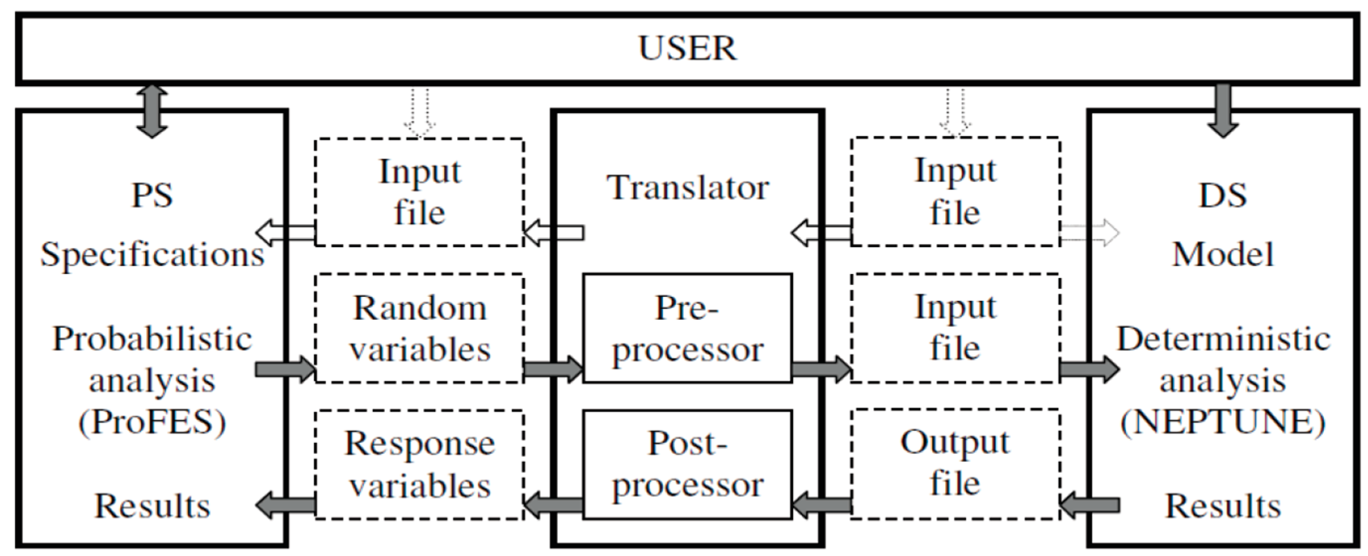
During translator execution, the values of random variables in the DS input file are typically adjusted based on values determined by the PS. Additionally, it retrieves response variable values from the DS output file for probabilistic analysis by the PS. After computations, the PS generates an analysis report presenting the results of the probabilistic analysis. Figure 1 illustrates the interactions among the user, PS, DS, and the translator, which comprises both a pre-processor and post-processor.
Initiating the integration process involves launching the probabilistic software (PS), which seamlessly incorporates the deterministic software (DS). The analyst proceeds by importing the DS model into the PS through a dedicated import interface. The configuration of the probabilistic model ensues, encompassing tasks such as selecting random variables, specifying distributions, setting correlations, and defining dependent variables and limit states. The specifics of this configuration hinge on the nature of the intended probabilistic analysis.
Typically, the identification of random variables and their respective distributions, along with parameter specification, forms a pivotal aspect of the probabilistic model setup. These variables are derived from quantities in the DS deemed as changeable or random, as outlined in the input files. Before each DS calculation, the translator intervenes, adjusting values in the DS input file to align with those selected by the PS. Simultaneously, a list of response variables is delineated, corresponding to desired output quantities (e.g., displacements, stresses, and strain) that are pivotal for calculating failure parameters (e.g., failure rate and probability of failure) in the final analysis.
In practical terms, probabilistic methods offer a robust means of gauging the impact of uncertainties in material properties, component geometry data, and loads on predicting structural reliability and performance. The coupling of validated NEPTUNE and ProFES software facilitated the probabilistic analysis of structural failure under transient loading conditions. ProFES, developed by ARA’s Southeast Division Computational Mechanics Group, emerged as a versatile tool for swift probabilistic model development, either independently or as an extension of deterministic models.
For the deterministic transient analysis of a structure subjected to dynamic loading using NEPTUNE, random variables selected by ProFES were employed. Notably, due to the incompatibility of NEPTUNE input/output formats with ProFES, a specialized coupling code named pnglue was devised at the Argonne National Laboratory. This Perl-based code adeptly extracts information from one text file and generates another, seamlessly aligning with the interactive nature of the software tools. During pnglue execution, the identified random variables in the NEPTUNE input file is dynamically adjusted based on ProFES-determined values. Subsequently, response variables are retrieved from the NEPTUNE output file, enabling ProFES to conduct a comprehensive probabilistic analysis. After the computations are completed, ProFES furnishes an analysis report encapsulating the outcomes of the probabilistic analysis.
Methodology for Integrated Analysis of Failures
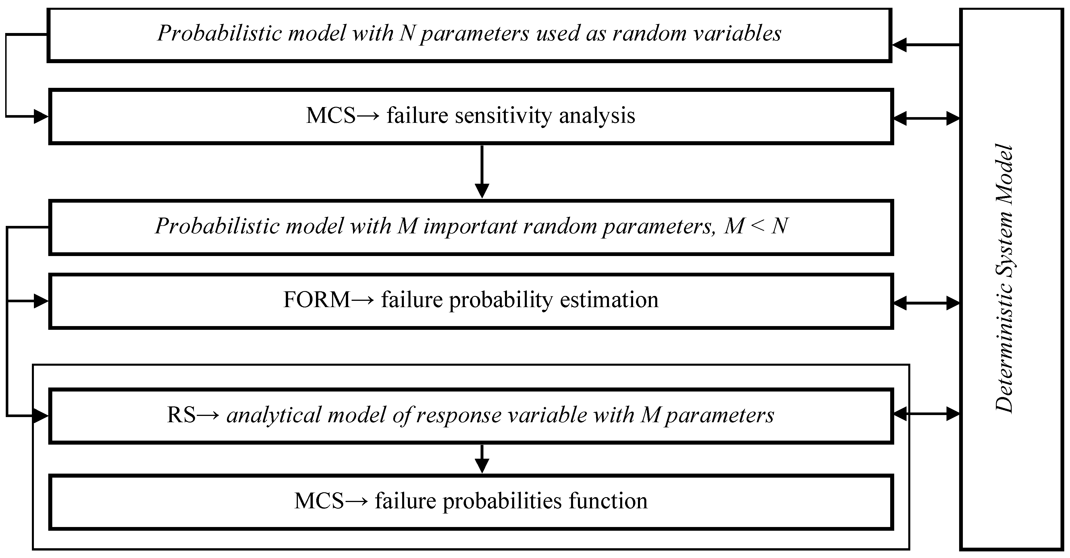
The proposed integrated failure analysis methodology involves combining multiple methods to obtain comprehensive insights. The Monte Carlo Simulation (MCS) method is initially employed to investigate the sensitivity of response variables and evaluate the influence of uncertainties in system properties and model parameters on the probability of encountering limit states, such as specific degradation conditions. Numerical uncertainties are treated as random variables with well-defined characteristics. Confidence ranges and subjective probability distributions are utilized to capture the state of knowledge on all uncertain parameters.
Focusing on the most critical parameters (as indicated in Figure 2 below), a more precise method, namely the First-Order Reliability Method (FORM), is then utilized to estimate the probability of failure in a complex system. Following this, to represent the failure probability as a function and explore the relationship between function parameters (e.g., load) and failure probability, the Response Surface/Monte Carlo Simulation (RS/MCS) method is employed.
By employing this methodology, the Monte Carlo Simulation method generates samples for each random variable, executing the deterministic model with various combinations of these variables. Estimates of uncertainties and probabilities are derived through a straightforward statistical analysis of the simulation results. This uncertainty analysis is designed to identify and quantify potentially significant uncertainty parameters.
As a primary sensitivity measure, the response sensitivity, denoting the derivative of the mean of the response variable Y concerning the mean of the random variable, is proposed for utilization. Subsequently, the screening of insignificant random variables from the extensive set of input random variables can be executed by applying 95% confidence limits to this sensitivity measure. These limits are suggested as the acceptance criteria for defining the most influential random variables for subsequent methods.
The magnitude of a sensitivity measure is directly proportional to the importance of the corresponding random variable. A random variable is deemed insignificant when its sensitivity measure is close to zero. If the sensitivity measure falls within the acceptance limits, it indicates that the random variable is likely insignificant. The employed sensitivity measure is denoted as , denoting the derivative of the mean of the response variable with respect to the mean of the input random variable . This particular sensitivity measure is accessible in Monte Carlo simulation-based methods, such as Monte Carlo simulation and the Response Surface with Monte Carlo Simulation method. The estimation of sensitivity using the Monte Carlo simulation method is articulated as follows:
Here is the number of simulations, is the evaluated response variable at the sampling point , and the last multiplier in the sum is the sensitivity of PDF at point .
In general, the sensitivity of PDF is determined by numerical differentiation (unless the analytic measure of sensitivity is available for the random variable with normal distribution) as:
As previously mentioned, for the same level of precision as Monte Carlo Simulation (MCS), the First-Order Reliability Method (FORM) is the preferred choice when evaluating small probabilities. This preference stems from the fact that the FORM often requires fewer finite element model runs. The computational effort in the FORM is directly proportional to the number of random variables and limit states.
In light of this, it is recommended to select the most crucial random variables and limit states based on the results obtained from MCS. Subsequently, the Response Surface/Monte Carlo Simulation (RS/MCS) method can be employed to establish a function that expresses the failure probability. Moreover, the RS/MCS method is suggested for exploring the relationship between failure probability and influential parameters.
For practical implementation details of this methodology, please refer to the subsequent section.
4. Example of the Applications of Integrated Methods for the Structural Integrity
The methodology presented here integrates probabilistic techniques with deterministic modeling based on the finite element method. It involves connecting a validated finite element software package to an established probabilistic package to conduct a comprehensive analysis of the intricate mechanics observed during transient nonlinear analyses of impact problems. This approach is specifically applied to a pipe whip analysis of a group distribution header, resulting from a guillotine break and subsequent impact with the adjacent group distribution header—a postulated accident scenario for the Ignalina Nuclear Power Plant RBMK-1500 reactors. The analysis takes into account uncertainties in material properties, component geometry data, and loads. The probabilities of failure for both the impacted header and the header support wall are estimated, considering the uncertainties in material properties, geometry parameters, and loading conditions.
4.1. Introduction Regarding the Case Study
The Ignalina Nuclear Power Plant houses two RBMK-1500 reactors, which are known for their unique design with a large number of pipes, particularly high-energy pipelines, situated nearby. The concern arises from potential guillotine ruptures in these high-energy pipelines, posing a significant risk to nearby pipelines and structural components. To assess the potential damage resulting from pipe ruptures, it is crucial to ensure that the building structures and adjacent components can withstand dynamic loading during a maximum design accident. Simultaneously, calculations need to determine whether the strength of the pipes is sufficient to prevent a single rupture from escalating into a multiple-rupture event, which is the focus of this paper.
The group distribution header (GDH) assumes a critical role in reactor safety by connecting to the Emergency Core Cooling System (ECCS) piping. In the event of a rupture, coolant surges through the ECCS and GDH piping, leading to additional loads. The GDH, set into motion after a guillotine break, can potentially collide with neighboring GDH components or the adjacent compartment wall.
This study presents a conservative analysis of the GDH pipe break transient [28], employing an integrated methodology that combines probabilistic methods with deterministic modeling through nonlinear finite element transient analysis. The deterministic modeling involves the application of validated NEPTUNE [6], a finite element software capable of analyzing dynamic pipe whip scenarios with significant displacements and nonlinear material responses. The focus is on modeling a whipping GDH, supporting concrete walls, and adjacent building walls.
For the probabilistic analysis associated with the same piping failure and wall damage resulting from the GDH guillotine failure, ProFES [11] software is employed. ProFES serves as a probabilistic analysis system, empowering designers to conduct probabilistic finite element analyses in a 3D environment, which is reminiscent of the modern deterministic FEA. The integration of ProFES with the deterministic finite element software NEPTUNE, as elaborated in [7], facilitates the modeling of uncertainty and its influence on model and system reliability. To conduct probabilistic analyses of the adjacent GDH and support wall in the event of a GDH guillotine break, the Monte Carlo Simulation method, First-Order Reliability Method, and Response Surface method are deployed.
4.2. Model for the Analysis of Damage to the Adjacent Piping
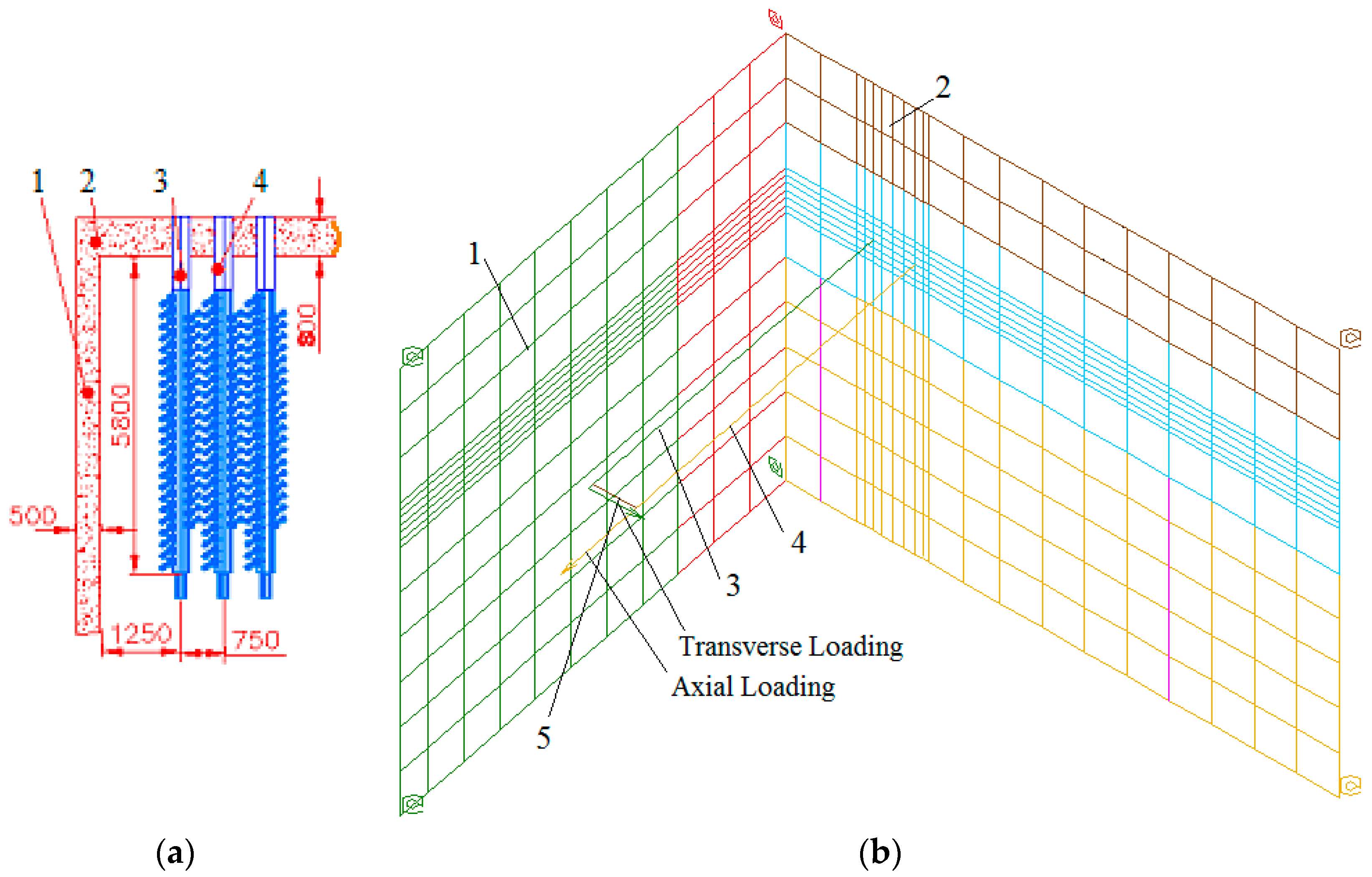
The GDH pipes are situated within the confines of the GDH compartment, with a small separation of 425 mm between two GDHs. The primary focus of the investigation lies in the collision between these adjacent GDH pipelines. Given the significance of the structural integrity of the GDH supporting wall, the model incorporates GDH pipes 3 and 4 along with walls 1 and 2 (refer to Figure 3a) [28]. The group distribution header takes the form of a horizontal cylinder with an external diameter of 325 mm, a wall thickness of 15 mm, and a length of approximately 5 m.
For the analysis of GDH’s impact on the adjacent GDH pipe following a GDH guillotine failure, a combined model of GDH pipes and concrete walls is employed. The finite-element model of the GDH encompasses two GDH pipelines, associated piping, and two neighboring concrete walls, as illustrated in Figure 3b.
The compartment walls were modeled using the four-node quadrilateral plate element developed by Belytschko et al. [29]. This element’s formulation is rooted in the Mindlin theory of plates and incorporates a velocity strain formulation, enabling elastoplastic behavior. Kulak and Fiala [6] extended the formulation to represent a composite plate of reinforced concrete. The GDHs were simulated using three-dimensional pipe elements to ensure a comprehensive solution for a pipe whip event, accounting for large displacements in three-dimensional space.
Regarding material properties, the analyzed model comprises two main components: the GDH, constructed from 08X18H10T steel, and the compartment walls, constructed from reinforced heavy concrete M300.
For an in-depth understanding of the geometry of the GDH, the adjacent piping, surrounding walls, material properties, finite element methodology, and additional details can be found in [28].
The transient analysis of a guillotine pipe break was previously expounded in [28], adopting a conservative assumption that the transverse load applied to the end of the GDH was equivalent to the axial load. This load, treated as an upper bound, was not considered a random variable in the Monte Carlo Simulation method nor the First-Order Reliability Method employed in this study; however, the precise magnitude of the guillotine break load remains uncertain. To address this uncertainty, the RS/MCS method was utilized to express the failure probability as a function of the loading and explore the correlation between the impact load and failure probability.
4.3. Data for Probabilistic Analysis
The objective of the uncertainty analysis is to identify and quantify all potentially significant uncertainty parameters. Ranges and subjective probability distributions are employed to describe the state of knowledge regarding these uncertain parameters. In probabilistic analyses, numerical uncertainties are modeled as random variables. The mechanical properties and geometrical parameters crucial to the structural strength are treated as random variables, including the following:
- Mechanical properties.
- Geometry data.
The material property test data for the reinforced concrete and GDH pipes are sourced from the Ignalina NPP. Given the limited quantity of tested samples, and insufficient statistical analyses, the coefficient of variation was adopted based on data and approaches presented in [30,31]. The logarithmic normal distribution was applied to the mechanical properties and geometry parameters in this analysis. The selected random variables (parameters), distributions, means, and non-dimensional coefficients of variation (COV = Std. Dev./Mean) are presented in Table 1 and Table 2.
4.4. Selected Limit States for Analysis
After a guillotine break, the investigation focused on the potential impact of a displaced GDH pipe on neighboring GDH pipes. The transient analysis aimed to assess the following:
- The structural integrity of adjacent GDHs after impact.
- The structural integrity of the GDH-supporting wall.
The following limit states were considered for the case of GDH impact on adjacent GDHs:
- Limit State 1: contact between the broken group distribution header and the adjacent pipe.
- Limit States 2, 3, 4, 5, and 6: The concrete adjacent to the group distribution header fixity in the support wall reaches the ultimate strength for compression and loses resistance to further loading. The same limit states at all five integration points through the wall thickness were checked.
- Limit State 7, 8, 9, 10: The strength limit of the first layer of rebars in the concrete support wall at the location of the group distribution header fixity is reached, and the rebars can fail. The same limit states at all four layers were checked in the analysis using the MCS method. In the case of the FORM, the computational effort is proportional to the number of random variables and limit states. The probabilities of the failure of all rebar layers were received as ridiculously small and similar to the MCS analysis. Therefore, Limit State 7 (the strength limit of the first layer of rebars) was used in the analysis using the FORM.
- Limit State 11: The impacted GDH pipe element reaches the ultimate strength of pipe steel, and the pipe will be destroyed.
It is crucial to simultaneously calculate the probability of concrete element failure at all five integration points and the probability of reinforcement bar element failure across all four layers. Hence, two system events were utilized in the probability analysis:
- System Event 1—Comprising Limit State 2, Limit State 3, Limit State 4, Limit State 5, and Limit State 6. This system event is considered true if all the limit states are true, evaluating the probability of concrete failure at all integrated points.
- System Event 2—Encompassing Limit State 7, Limit State 8, Limit State 9, and Limit State 10. Similar to System Event 1, this event is true if all the corresponding limit states are true. It assesses the probability of rebar failure across all layers.
4.5. Probabilistic Analysis Results
The probabilistic analysis results using the Monte Carlo Simulation method, First-Order Reliability Method, and Response Surface method are presented in this section.
4.5.1. Probabilistic Analysis Using MCS Method
Monte Carlo Simulation was employed to investigate the impact of uncertainty in material properties and geometry parameters and to compute the probabilities of limit states. Just for demonstration purposes (assuming a computationally intensive model), a total of 300 simulations were conducted. It is essential to note that due to the relatively small number of Monte Carlo Simulations, the probabilistic analysis using the MCS method was carried out as a scoping study. Consequently, detailed results related to failure probability are not provided in this subsection. For a more accurate determination of probabilities, the FORM method was subsequently utilized. The objective of the uncertainty analysis is to identify and quantify all potentially significant uncertainty parameters, with ranges and subjective probability distributions characterizing the state of knowledge regarding these uncertainties.
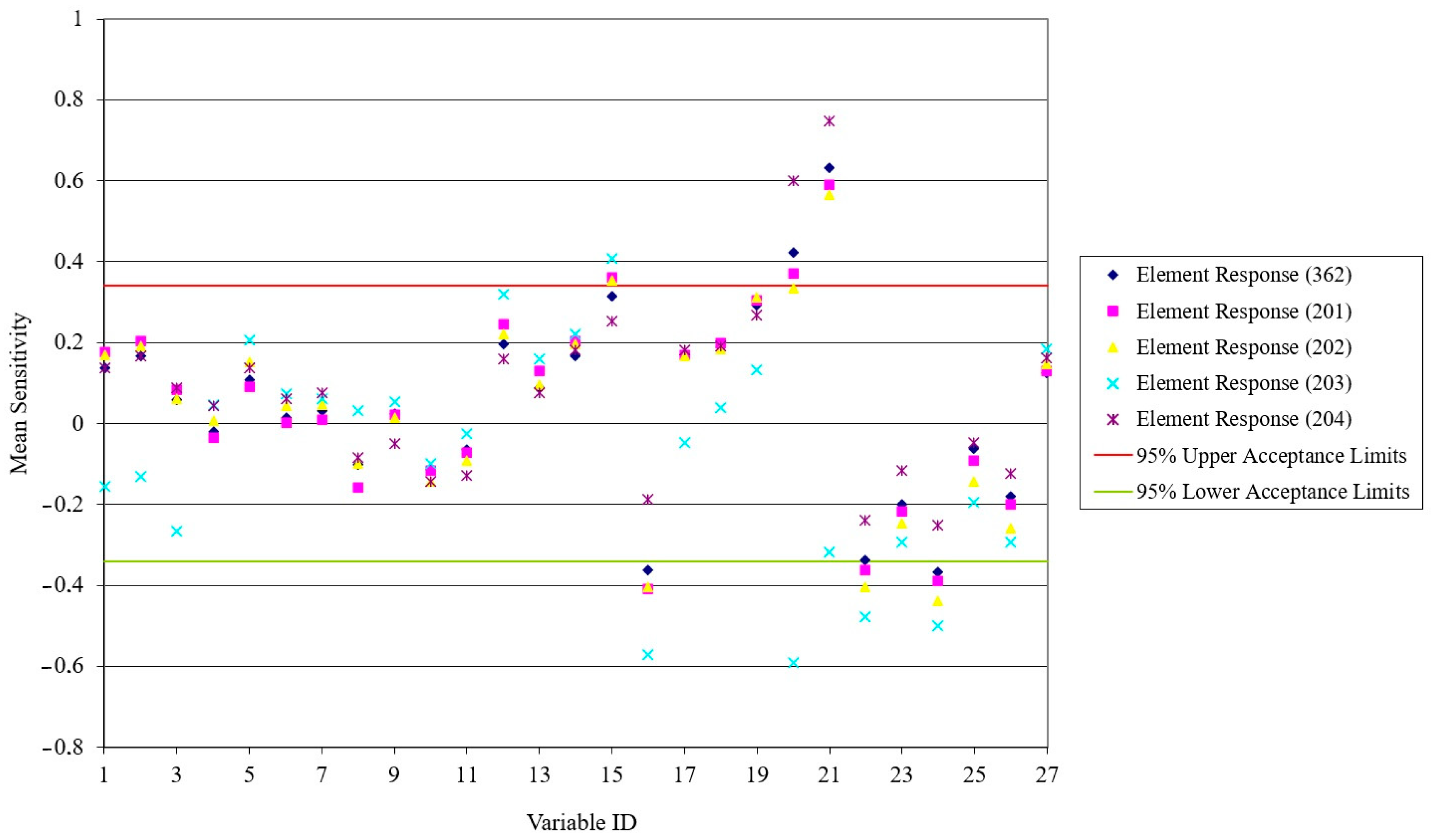
A logarithmic normal distribution was employed to model the material properties and geometry parameters for this analysis. Utilizing this probabilistic analysis method, the probabilities of limit states were computed, and a sensitivity analysis of material properties and geometry parameters was conducted. While twenty-seven random variables were initially considered (based on the parameters from a specific system model case), only the significant ones are discussed here. The screening of insignificant random variables from the extensive set was performed using 95% confidence limits for sensitivity measures, which served as acceptance limits for the corresponding random variables. To facilitate comparison across different values, the sensitivity measures and 95% confidence limits were normalized.
The specified input random variables (362, 201, 202, 203, and 204—Figure 4; 362 involves several concrete elements adjacent to the node of pipe fixity in the wall, while the numbers 201, 202, 203, and 204 are only the conditional designation of different integration points of 362 elements) are considered significant for Element Response Stress Equivalent:
- The rebar input variable of the supporting wall (2 in Figure 3)—input random variable 15.
- The yield stress of the reinforcement rebars of the supporting wall (2 in Figure 3)—input random variable 16.
- The thickness of the broken GDH pipe (3 in Figure 3)—input random variable 20.
- The mid-surface radius of the broken GDH pipe (3 in Figure 3)—input random variable 21.
- The Young’s modulus of the impacted GDH pipe (4 in Figure 3)—input random variable 22.
- The yield stress of the impacted GDH pipe (4 in Figure 3)—input random variable 24.
These input random variables possess the most significant positive or negative influence on all integration points of the support-wall concrete element number 362.
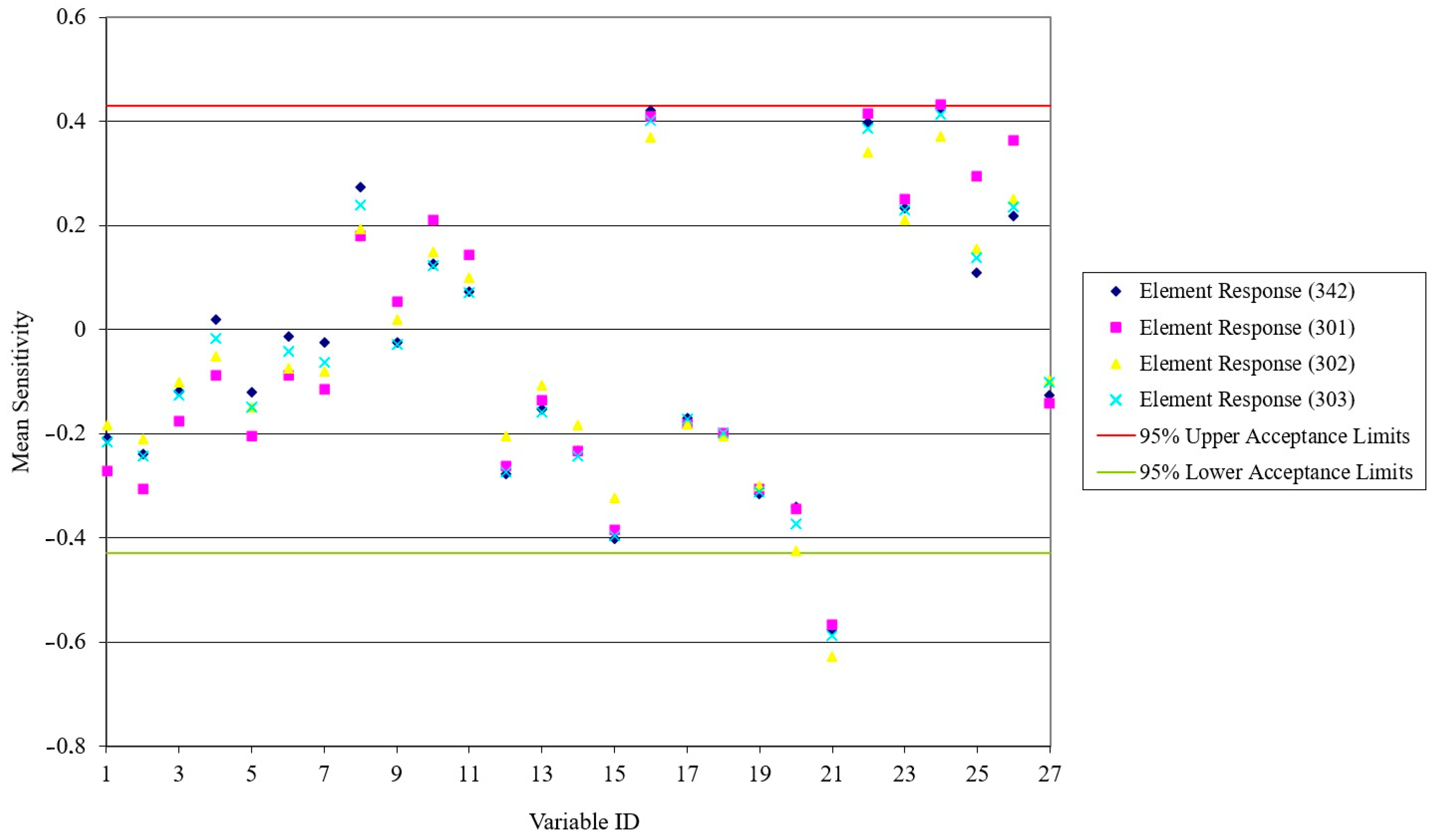
The specified input random variables (342, 301, 302, and 303—Figure 5; 342 is the number of concrete rebar elements adjacent to the node of the group distribution header fixity in the concrete support wall in layer 1, while the numbers 301, 302, and 303 are only the conditional designation of different integration points of 322 elements in layers 2, 3, and 4) are considered significant for Element Response Stress Equivalent:
These input random variables exert the most significant positive or negative influence on all layers of reinforcement rebars in concrete element number 342.
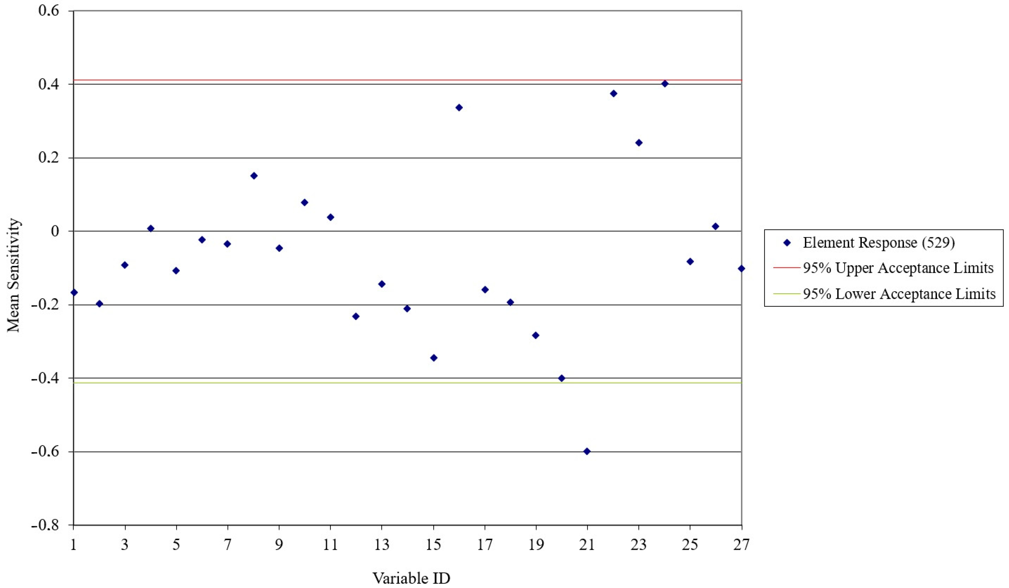
The specified input random variables (529—Figure 6) are considered significant for Element Response Stress Equivalent:
These input random variables exert the most significant positive impact (24) and negative impact (21) on the affected pipe element number 529.
According to the presented results, the following input random variables (conservatively including the nearest to acceptance limits of 95%) were also used in the FORM analysis as input random variables:
- The yield stress of the broken GDH pipe (3 in Figure 3)—input random variable 19.
- The rebar area of the supporting wall (2 in Figure 3)—input random variable 12.
- The Poisson’s ratio of the impacted GDH pipe (4 in Figure 3)—input random variable 23.
- The mid-surface radius of the impacted GDH pipe (4 in Figure 3)—input random variable 26.
- The rebar area of the supporting wall (2 in Figure 2)—input random variable 14.
- The Poisson’s ratio of the concrete of the supporting wall (2 in Figure 3)—input random variable 1.
- The Young’s modulus of the concrete of the supporting wall (4 in Figure 3)—input random variable 2.
All the random variables previously listed were utilized in the FORM analysis as input variables. This means that if the analyst is not sure about the outliers for further analysis, they can include some of the variables that are closest to the limit. Conservatively, we may include not only the variables strictly based on the interval but also those based on the variables, which are almost in the interval ranges (i.e., the nearest to the acceptance limit of 95%).
4.5.2. Probabilistic Analysis Applying the FORM
The FORM was utilized to evaluate the probability of failure for the impacted GDH pipe and supporting wall. The FORM stands out as the preferred approach for assessing small probabilities associated with concrete, reinforcement bars, and GDH pipe failure. This preference arises from the fact that, in order to achieve the same level of precision as Monte Carlo Simulation (MCS), FORM typically necessitates the fewest finite element model runs. As mentioned earlier, the computational effort in the FORM is directly tied to the number of random variables and limit states. Hence, the most crucial random variables and limit states were chosen based on the outcomes derived from MCS, as detailed in Section 4.5.1. The mechanical properties and geometrical parameters that significantly influence the strength of structures were designated as random variables in the FORM analysis, guided by the sensitivity analysis results from MCS.
The same limit states considered in the MCS analysis (Section 4.4) were adopted for the FORM analysis.
The FORM was utilized to perform a probabilistic analysis of the structural integrity of both the adjacent GDH after an impact and the supporting wall of the GDH. A log-normal distribution of the material properties and geometry data was employed for this analysis (refer to Table 1 and Table 2). Through this probabilistic analysis method, the probabilities of limit states were computed. The outcomes of the probabilistic analysis are detailed in Table 3 and Table 4.
It was determined that the probability of “Limit State 1” is 0.506. This probability indicates that the contact between two GDH pipes will occur with a likelihood of 0.506.
For the support wall (concrete element number 362, representing the adjacent concrete elements to the node of the whipping group distribution header pipe fixity), the computed probabilities for “Limit States 2, 3, 4, 5, and 6” vary between 0.474 and 0.503 (refer to Table 3). These limit states indicate that there is a possibility of reaching the ultimate compressive strength of concrete at the five integration points, potentially resulting in failure. The system event was employed to analyze the probability of failure simultaneously at all integration points of the concrete element during the same computational run. The calculated probability of “System Event 1” is 0.0502 (see Table 4). Consequently, there is a probability of 0.0502 that the ultimate compressive strength of concrete will be reached, and the support wall will fail at the location where the group distribution header is attached with the same probability of 0.0502.
For the concrete rebar in the support wall (element 342, representing the number of rebar elements adjacent to the node of the whipping group-distribution-header pipe fixity), the calculated probabilities for “Limit States 7, 8, 9, and 10” range from 2.092 × 10⁻⁹ to 0.485 (Table 3). This limit state indicates that the ultimate stress of the rebars will be reached in layers 8, 9, and 10, and that these rebars may fail. The probability of failure for the first layer of concrete rebar is ridiculously small—close to zero (2.092 × 10⁻⁹). The system event was used for analyzing the probability of failure during the same computational run at all integration points of the concrete rebar element. The calculated probability of “System Event 2” is approximately 0 (Table 4). Thus, the ultimate stress of the concrete rebar has a ridiculously small probability of being reached, and the rebars in the support wall may fail with an equally small probability.
A probability of 0.288 for “Limit State 11” was obtained. This limit state means that the ultimate stress will be reached with a probability of 0.288 in the impacted GDH pipe element, and that this pipe can be destroyed with a probability of 0.288.
4.5.3. Probabilistic Analysis Using the RS/MCS Method
The magnitude of the transverse load resulting from a guillotine break is challenging to determine precisely. Given this uncertainty, estimating the probability of failure for the impacted neighboring wall due to the transverse load on the group distribution header is crucial. The Response Surface/Monte Carlo Simulation method was employed to express the failure probability as a function of the loading and investigate the relationship between the impact load and failure probability.
In the initial segment of the Response Surface/Monte Carlo Simulation analysis, the Response Surface method was utilized to establish dependence functions between the response variables and the input random variables, with 100 simulations conducted. According to the classical statistical approach, the confidence statement expresses the possible influence of the fact that only a limited number of simulations have been performed. For example, according to the Wilks’ formula and its interpretation [32], only 93 model runs are sufficient to have a (0.95, 0.95) statistical tolerance interval (upper and lower limits). So, 100 simulations (rounded for demonstration purposes) can be a possible case for computationally intensive models.
In the subsequent part of the analysis, the Monte Carlo Simulation method was employed to determine the probability of failure based on these dependence functions. The deterministic transient analysis of the whipping group distribution header incorporated the loading obtained from thermo-hydraulic analysis [28]. While this load was treated as an upper bound and deterministic in the Monte Carlo Simulation and First-Order Reliability Method studies, a different loading was utilized in the Response Surface part of the analysis.
The application case of the Response Surface/Monte Carlo Simulation method does not handle all the random variables related to the critical loading points at a different time; instead, it handles only one load value. Thus, a mean loading value was set as a constant, 338 kN in the range from 0.00 s up to 0.012 s, followed by zero thereafter. This load value represents half of the maximum load value (677 kN). A uniform distribution was applied for loadings in the Response Surface part of the analysis, ranging from 0 N to the maximum loading of 677 kN.
The same mechanical properties and geometrical parameters identified as crucial for the strength of structures were selected as random variables. Logarithmic normal distributions of material properties and geometry parameters were used for this analysis, and the same limit states (as described in Section 4.4) were applied in the Response Surface/Monte Carlo Simulation analysis as those used in the Monte Carlo Simulation and First-Order Reliability Method analysis.
Utilizing the Response Surface method, the dependence functions between response variables and input random variables were computed. In the subsequent part of the Response Surface/Monte Carlo Simulation analysis, specifically the Monte Carlo method, these functions were employed to ascertain the failure probability.
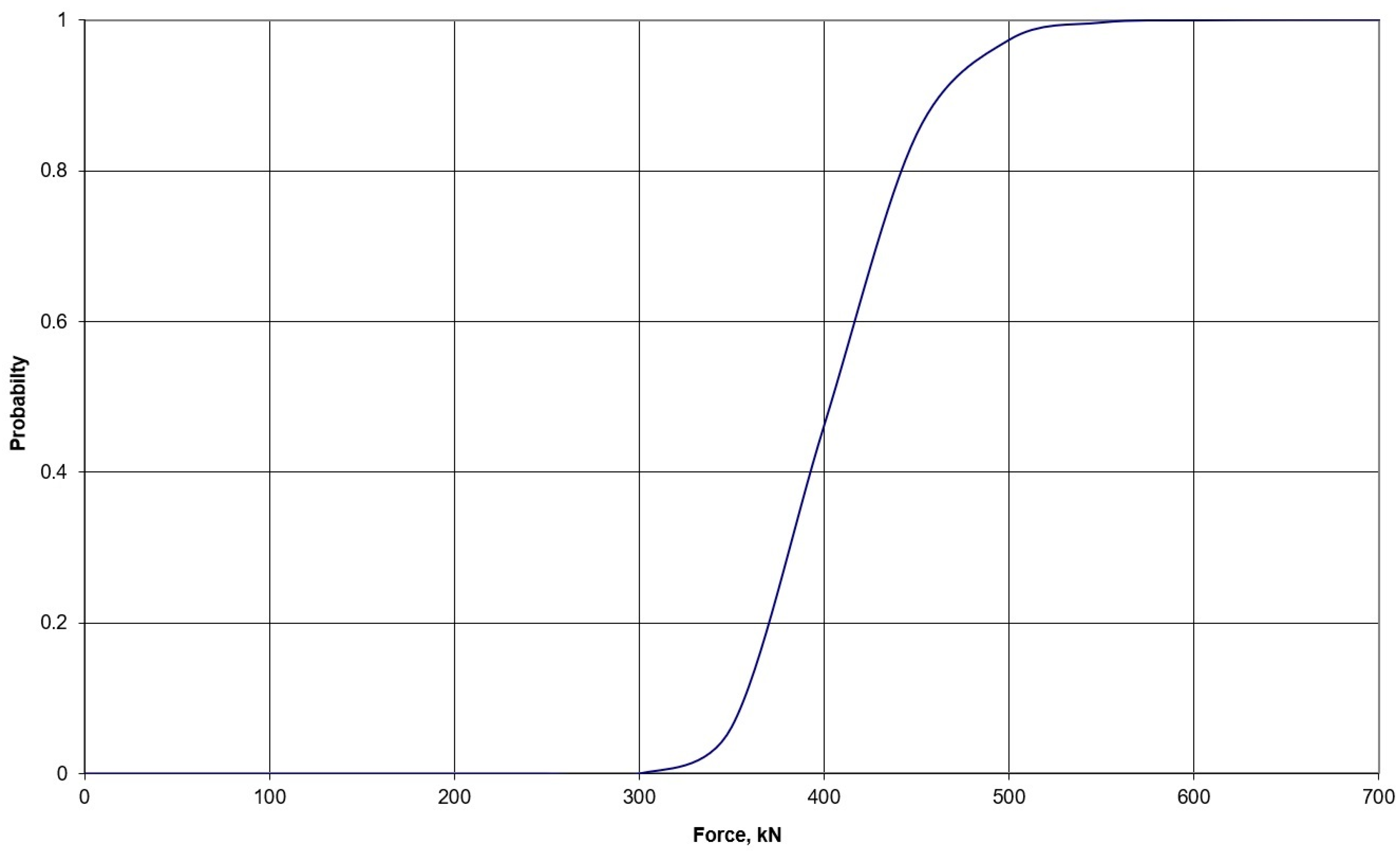
The probability-loading function was established for the ultimate compressive strength of concrete in the support wall. The equation derived from the Response Surface analysis to determine the failure probability for Limit State 2 (refer to Table 3)—“Element Response (362 is the element number, first integration point) Stress Equivalent > 1.7 × 10⁷”—is as follows:
y = (−5.35995 × 10⁷) + (18.6745 × L11-1)+ (9.04392 × L11-3) + (5.85753 × 10⁷ × P4) + (−0.000360327 × Y4) +
(−7.24406 × 10⁹ × re1) + (−1.03215 × 10⁹ × re3) + (1.22263 × 10¹⁰ × re4) + (0.0081826 × r5) +
(0.00255908 × Yi7) + (6.88826 × 10⁸ × t7) + (1.22627 × 10⁸ × m7) + (−0.000177385 × Y8) +
(8.63534 × 10⁷ × P8) + (0.0239527 × Yi8) + (5.77211 × 10⁷ × m8).
(−7.24406 × 10⁹ × re1) + (−1.03215 × 10⁹ × re3) + (1.22263 × 10¹⁰ × re4) + (0.0081826 × r5) +
(0.00255908 × Yi7) + (6.88826 × 10⁸ × t7) + (1.22627 × 10⁸ × m7) + (−0.000177385 × Y8) +
(8.63534 × 10⁷ × P8) + (0.0239527 × Yi8) + (5.77211 × 10⁷ × m8).
Here, the response variable “y” is incorporated into the limit state condition y > −1.7 × 10⁷. L11-1 is the Load Unit 1-1, and L11-3 is the Load Unit 1-3 (Load Unit 1-1 and Load 1-3 are loading points at different times). P4 is the Poisson’s ratio of wall 2 (Figure 3), Y4 is the Young’s modulus of the concrete of wall 2, re1 is the rebar 1 area of wall 2, re3 is the rebar 3 area of wall 2, re4 is the rebar 4 area of wall 2, r5 is the yield stress of the reinforcement bar in wall 2, Yi7 is the yield Stress of pipe 3, t7 is the thickness of pipe 3, m7 iks the mid-surface radius of pipe 3, Y8 is the Young’s modulus of pipe 4, P8 is the Poisson’s ratio of pipe 4, Yi8 is the yield Stress of pipe 4, and m8 is the mid-surface radius of pipe 4.
In Equation (10), loads L1 and L3 were assumed to be equal, and they were changed incrementally while observing the corresponding changes in the probability of the limit state, ranging from 0 to 1. The normal distribution with a coefficient of variation of 0.1 (10%) for loading, and the logarithmic normal distribution for material properties and geometry parameters, were applied in this analysis. The nominal values of material properties and geometry parameters in Equation (5) remained consistent with those used in other analyses. The analysis data are visually presented in Figure 7, illustrating the relationship between the probability of “Limit State 2” and the applied loads. Notably, concrete element 362′s ultimate compressive strength according to Equation (10) is reached at an approximate loading of 300 kN (for a demonstration, see Figure 7), with the probability of concrete failure in layer 1 becoming 1 at a loading of approximately 550 kN.
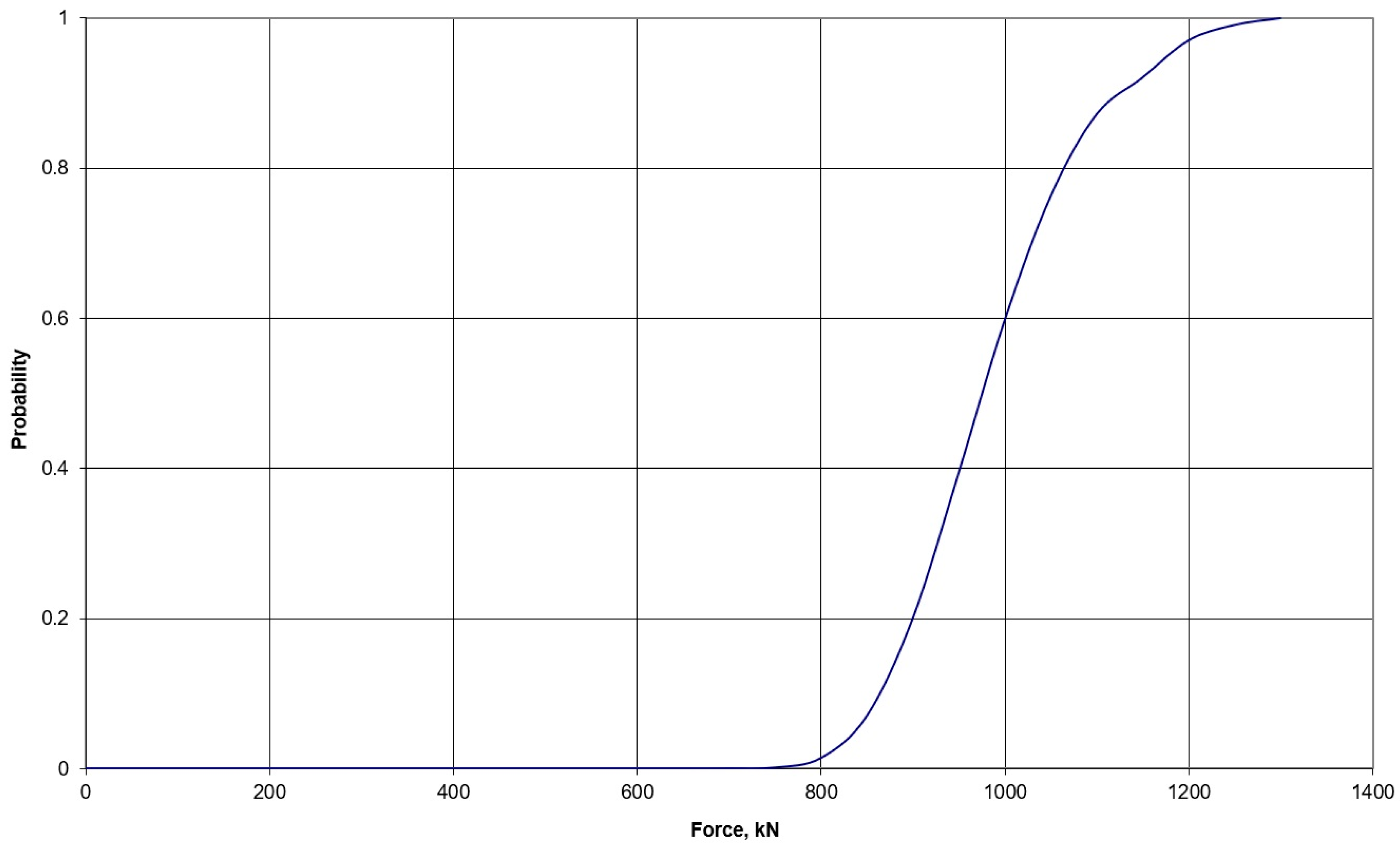
The equation derived from the Response Surface analysis to calculate the failure probability of Limit State 11 (Table 3)—“Element Response (529 is the element number of impacted GDH, Stress Equivalent > 412,000,000”—is as follows:
y = (1.23357 × 10⁸) + (−177.237 × L11-1) + (−204.367 × L11-3) + (−4.85967 × 10⁸ × P4) + (0.00103062 × Y4) +
(5.94666 × 10¹⁰ × re1) + (−4.37383 × 10¹⁰ × re3) + (−3.91527 × 10⁹ × re4) + (−0.357241 × r5) +
(0.0785711 × Yi7) + (−7.64796 × 10⁸ × t7) + (−9.9672 × 10⁷ × m7) + (0.00315964 × Y8) +
(−5.69678 × 10⁸ × P8) + (0.051506 × Yi8) + (−1.04162 × 10⁹ × m8).
(5.94666 × 10¹⁰ × re1) + (−4.37383 × 10¹⁰ × re3) + (−3.91527 × 10⁹ × re4) + (−0.357241 × r5) +
(0.0785711 × Yi7) + (−7.64796 × 10⁸ × t7) + (−9.9672 × 10⁷ × m7) + (0.00315964 × Y8) +
(−5.69678 × 10⁸ × P8) + (0.051506 × Yi8) + (−1.04162 × 10⁹ × m8).
The same variables are explained below Equation (10).
The results of the analysis are depicted in Figure 8, illustrating the relationship between the probability of “Limit State 11” and the applied loads. According to these findings, the ultimate stress (based on Equation (11)) in impacted GDH pipe element 529 reaches a loading of approximately 750 kN (for a demonstration, see Figure 8). The pipe failure probability becomes 1 at a loading of around 1300 kN.
5. Summary and Conclusions
A probability-based approach integrating deterministic and probabilistic methods was developed for the analysis of building and component failures in complex structures. The methodology links an existing and validated finite element software package with a probabilistic package, making it applicable to diverse systems like nuclear power plants and pipeline networks. This approach is crucial for structures with potential environmental risks upon failure.
In a case study demonstrating this methodology, a deterministic transient analysis was conducted using the finite element method (NEPTUNE software) for a guillotine break of a group distribution header. Probabilistic models (ProFES software) specified values for random variables, enabling numerous deterministic analyses with varied input parameters. ProFES then facilitated probabilistic analyses of piping failures and wall damage.
Probabilistic methods, including Monte Carlo Simulation (MCS), the First-Order Reliability Method (FORM), and a method combining MCS with Response Surface, were employed to assess failure probabilities under severe transient loading. For the Ignalina Nuclear Power Plant case study, uncertainties in material properties, geometry, and loads were considered, resulting in the estimation of probabilities of failure for the impacted header and support wall.
MCS was utilized to explore sensitivity, evaluating the impact of uncertainties on the limit states and failure probabilities. The FORM focused on estimating failure probabilities, demonstrating conservatism for large values but limitations for small probabilities. The Response Surface/Monte Carlo Simulation (RS/MCS) method was employed to express the failure probability as a function and explore the relationship between the impact load and failure probability.
The results revealed that given the substantial uncertainties in material properties and loadings in complex structures, deterministic analyses alone are insufficient. Probabilistic analyses, as demonstrated, are imperative for credible evaluations of structural safety during extreme loading events in complex systems like nuclear power plants.
Author Contributions
Conceptualization, R.A. and G.D.; methodology, R.A.; software, R.A. and G.D.; formal analysis, R.A. and G.D.; investigation, R.A. and G.D.; resources, R.A. and G.D.; data curation, R.A. and G.D.; writing—original draft preparation, R.A. and G.D.; writing—review and editing, R.A. and G.D.; supervision, R.A.; project administration, R.A.; funding acquisition, R.A. All authors have read and agreed to the published version of the manuscript.
Funding
This research received no external funding.
Data Availability Statement
Data are contained within the article.
Acknowledgments
The authors express their gratitude for the support and access to the latest NEPTUNE software, which was generously provided by the U.S. Department of Energy and the Argonne National Laboratory. Similarly, the authors are thankful for being granted access to ProFES, which was developed by U.S. Applied Research Associates (ARA) Inc., ARA’s Southeast Division Computational Mechanics Group. It is important to note that the U.S. Government does not endorse the results of this work. The authors thank anonymous reviewers and editors for their careful reading of our manuscript and their insightful comments and suggestions to improve the paper.
Conflicts of Interest
The authors declare no conflicts of interest.
References
- Youn, B.D.; Choi, R.-J.; Gu, L. Reliability-Based Design Optimization for Crashworthiness of Vehicle Side Impact. Struct. Multidiscip. Optim. 2004, 26, 272–283. [Google Scholar] [CrossRef]
- Padula, S.; Gumbert, C.; Li, W. Aerospace Applications of Optimization under Uncertainty. Optim. Eng. 2006, 7, 317–328. [Google Scholar] [CrossRef]
- Alzbutas, R.; Dundulis, G.; Kulak, R. Finite element system modeling and probabilistic methods application for structural safety analysis. In Proceedings of the 3rd Safety and Reliability International Conference KONBiN’03: Conference, Proceedings, Gdynia, Poland, 27–30 May 2003; Volume N3, pp. 213–220, ISBN 1642-9311. [Google Scholar]
- Lyle, K.H.; Stockwell, A.E.; Hardyr, R.C. Application of probability methods to assess airframe crash modeling uncertainty. J. Aircr. 2007, 44, 1568–1573. [Google Scholar] [CrossRef]
- Almenas, K.; Kaliatka, A.; Uspuras, E. Ignalina RBMK-1500. A Source Book. Extended and Updated Version; Ignalina Safety Analysis Group, Lithuanian Energy Institute: Kaunas, Lithuania, 1998. [Google Scholar]
- Kulak, R.F.; Fiala, C. Neptune a System of Finite Element Programs for Three Dimensional Nonlinear Analysis. Nucl. Eng. Des. 1988, 106, 47–68. [Google Scholar] [CrossRef]
- Kulak, R.F.; Marchertas, P. Development of a Finite Element Based Probabilistic Analysis Tool. In Proceedings of the 17th International Conference on Structural Mechanics in Reactor Technology, Prague, Czech Republic, 17–22 August 2003. Paper B215. [Google Scholar]
- Song, J.; Kang, W.H.; Lee, Y.J.; Chun, J. Structural system reliability: Overview of theories and applications to optimization. ASCE-ASME J. Risk Uncertain. Eng. Syst. Part A Civ. Eng. 2021, 7, 03121001. [Google Scholar] [CrossRef]
- Zhang, J. Modern Monte Carlo methods for efficient uncertainty quantification and propagation: A survey. WIREs Comput. Stat. 2021, 13, e1539. [Google Scholar] [CrossRef]
- Zhou, S.; Zhang, J.; Zhang, Q.; Huang, Y.; Wen, M. Uncertainty Theory-Based Structural Reliability Analysis and Design Optimization under Epistemic Uncertainty. Appl. Sci. 2022, 12, 2846. [Google Scholar] [CrossRef]
- Wu, Y.-T.; Shin, Y.; Sues, R.H.; Cesare, M.A. Probabilistic function evaluation system (ProFES) for reliability-based design. Struct. Saf. 2006, 28, 164–195. [Google Scholar] [CrossRef]
- Kunstmann, H.; Kinzelbach, W.; Siegfried, T. Conditional first-order second-moment method and its application to the quantification of uncertainty in groundwater modeling. Water Resour. Res. 2002, 38, 6/1–6/14. [Google Scholar] [CrossRef]
- Zhang, J.; Cui, S. Investigating the Number of Monte Carlo Simulations for Statistically Stationary Model Outputs. Axioms 2023, 12, 481. [Google Scholar] [CrossRef]
- Liel Abbie, B.; Haselton Curt, B.; Deierlein Gregory, G.; Baker Jack, W. Incorporating modeling uncertainties in the assessment of seismic collapse risk of buildings. Struct. Saf. 2009, 31, 197–211. [Google Scholar] [CrossRef]
- Wang, Z.; Zhang, Y.; Song, Y. An Adaptive First-Order Reliability Analysis Method for Nonlinear Problems. Math. Probl. Eng. 2020, 2020, 3925689. [Google Scholar] [CrossRef]
- Shittu, A.A.; Kolios, A.; Mehmanparast, A. A Systematic Review of Structural Reliability Methods for Deformation and Fatigue Analysis of Offshore Jacket Structures. Metals 2021, 11, 50. [Google Scholar] [CrossRef]
- Yin, J.; Du, X. High-Dimensional Reliability Method Accounting for Important and Unimportant Input Variables. ASME J. Mech. Des. 2022, 144, 041702. [Google Scholar] [CrossRef]
- García-Soto, A.-D.; Calderón-Vega, F.; Mösso, C.; Valdés-Vázquez, J.-G.; Hernández-Martínez, A. Revisiting Two Simulation-Based Reliability Approaches for Coastal and Structural Engineering Applications. Appl. Sci. 2020, 10, 8176. [Google Scholar] [CrossRef]
- Low, B.K.; Boon, C.W. Probability-Based Design of Reinforced Rock Slopes Using Coupled FORM and Monte Carlo Methods. Rock Mech. Rock Eng. 2023, 57, 1195–1217. [Google Scholar] [CrossRef]
- Hu, Z.; Mansour, R.; Olsson, M.; Du, X. Second-order reliability methods: A review and comparative study. Struct. Multidisc. Optim. 2021, 64, 3233–3263. [Google Scholar] [CrossRef]
- Ditlevsen, O.; Madsen, H.O. Structural Reliability Methods; Jon Wiley & Sons, Inc.: Chichester, UK, 2007; Volume 1, ISBN 0 471 96086 1. [Google Scholar]
- Chun, J. Reliability-Based Design Optimization of Structures Using Complex-Step Approximation with Sensitivity Analysis. Appl. Sci. 2021, 11, 4708. [Google Scholar] [CrossRef]
- Sues, R.H.; Cesare, M.A. System reliability and sensitivity factors via the MPPSS method. Probabilistic Eng. Mech. 2005, 20, 148–157. [Google Scholar] [CrossRef]
- El Hajj Chehade, F.; Younes, R. Structural reliability software and calculation tools: A review. Innov. Infrastruct. Solut. 2020, 5, 29. [Google Scholar] [CrossRef]
- Hadiyat, M.A.; Sopha, B.M.; Wibowo, B.S. Response Surface Methodology Using Observational Data: A Systematic Literature Review. Appl. Sci. 2022, 12, 10663. [Google Scholar] [CrossRef]
- Jankovic, A.; Chaudhary, G.; Goia, F. Designing the design of experiments (DOE)—An investigation on the influence of different factorial designs on the characterization of complex systems. Energy Build. 2021, 250, 111298. [Google Scholar] [CrossRef]
- Kim, C.; Choi, K.K. Reliability-Based Design Optimization Using Response Surface Method With Prediction Interval Estimation. ASME J. Mech. Des. 2008, 130, 121401. [Google Scholar] [CrossRef]
- Dundulis, G.; Ušpuras, E.; Kulak, R.F.; Marchertas, A. Evaluation of pipe whip impacts on neighboring piping and walls of the Ignalina Nuclear Power Plant. Nucl. Eng. Des. 2007, 237, 848–857. [Google Scholar] [CrossRef]
- Belytschko, T.; Lin, J.I.; Tsay, C.S. Explicit Algorithms for Nonlinear Dynamics of Shells. Comput. Methods Appl. Mech. Eng. 1984, 42, 225–251. [Google Scholar] [CrossRef]
- Low, H.Y.; Hao, H. Reliability analysis of reinforced concrete slabs under explosive loading. Struct. Saf. 2001, 23, 157–178. [Google Scholar] [CrossRef]
- Braverman, J.I.; Miller, C.A.; Ellingwood, B.R.; Naus, D.J.; Hofmayer, C.H.; Bezler, P.; Chang, T.Y. Structural Performance of Degraded Reinforced Concrete Members. In Proceedings of the 17th International Conference on Structural Mechanics in Reactor Technology, Washington, DC, USA, 12–17 August 2001. [Google Scholar]
- Hofer, E. Sensitivity analysis in the context of uncertainty analysis for computationally intensive models. Comput. Phys. Commun. 1999, 117, 21–34. [Google Scholar] [CrossRef]
Figure 1.
Integration of models and probabilistic methods.

Figure 2.
The integration of diverse probabilistic failure analysis.

Figure 3.
The top view of the GDHs within the compartment (a) and the integrated model comprising GDH pipes and concrete walls (b) for examining the impact on piping is depicted as follows: 1—adjacent wall; 2—GDH’s support wall; 3—broken GDH; 4—impacted GDH pipe; and 5—contact element between GDH pipes.

Figure 4.
Significant random variables (362, 201, 202, 203, and 204) for Element Response Stress Equivalent.
Figure 4.
Significant random variables (362, 201, 202, 203, and 204) for Element Response Stress Equivalent.

Figure 5.
Significant random variables (342, 301, 302, and 303) for Element Response Stress Equivalent.
Figure 5.
Significant random variables (342, 301, 302, and 303) for Element Response Stress Equivalent.

Figure 6.
Significant random variable (529) for Element Response Stress Equivalent.

Figure 7.
The probability of concrete failure under dynamic loading caused by a guillotine rupture.

Figure 8.
The failure probability of impacted GDH pipe at dynamic loading due to guillotine rupture.
Figure 8.
The failure probability of impacted GDH pipe at dynamic loading due to guillotine rupture.


Table 1.
Material properties and parameters (represented as random variables).
| Material/ Location | Parameter | Distribution | Mean | Unit | COV |
|---|---|---|---|---|---|
| Reinforced Concrete | |||||
| Concrete (walls 1 and 2 in Figure 3) | Poisson’s ratio | Log-normal | 0.2 | - | 0.10 |
| Young’s modulus | Log-normal | 2.7 × 10¹⁰ | Pa | 0.10 | |
| Uniaxial tensile strength | Log-normal | 1.5 × 10⁶ | Pa | 0.10 | |
| Reinforcement bars (walls 1 and 2) | Yield stress | Log-normal | 3.9 × 10⁸ | Pa | 0.03 |
| GDH Pipe | |||||
| Austenitic Steel (pipes 3 and 4 in Figure 3) | Young’s modulus | Log-normal | 1.8 × 10¹¹ | Pa | 0.03 |
| Poisson’s ratio | Log-normal | 0.3 | - | 0.03 | |
| Yield stress | Log-normal | 1.8 × 10⁸ | Pa | 0.03 | |
| Contact of Pipes | Contact modulus | Normal | 1.8 × 10¹¹ | Pa | 0.10 |
Table 2.
The geometry parameters as random variables.
| Material/Location | Parameter | Distribution | Mean | Unit | COV |
|---|---|---|---|---|---|
| Reinforced Concrete | |||||
| Reinforcement bars | Reinforcement layer thickness (data are presented for 1 rebar) | Log-normal | 0.0031 | m | 0.05 |
| GDH Pipe | |||||
| Austenitic steel | Wall thickness | Log-normal | 0.0015 | m | 0.05 |
| The mid-surface radius of the pipe | Log-normal | 0.1550 | m | 0.05 | |
Table 3.
Results related to each limit state.
| Name * | Definition * | Probability | Beta, See (6) |
|---|---|---|---|
| LS 1 | NR (572) DD 2 (Y) < −0.425 | 0.506254 | 0.0156768 |
| LS 2 | ER (362) SE < −1.7 × 10⁷ | 0.500205 | 0.0005131 |
| LS 3 | ER (201) SE < −1.7 × 10⁷ | 0.503351 | 0.0083994 |
| LS 4 | ER (202) SE < −1.7 × 10⁷ | 0.474443 | −0.0641049 |
| LS 5 | ER (203) SE < −1.7 × 10⁷ | 0.499217 | −0.0019636 |
| LS 6 | ER (204) SE < −1.7 × 10⁷ | 0.498017 | −0.0049704 |
| LS 7 | ER (342) SE > 5.9 × 10⁸ | 2.092 × 10⁻⁹ | −5.8772800 |
| LS 8 | ER (301) SE > 5.9 × 10⁸ | 0.476667 | −0.0585204 |
| LS 9 | ER (302) SE > 5.9 × 10⁸ | 0.473746 | −0.0658572 |
| LS 10 | ER (303) SE > 5.9 × 10⁸ | 0.484998 | −0.0376143 |
| LS 11 | ER (529) SE > 4.12 × 10⁸ | 0.287865 | −0.5596310 |
* Where LS—limit state; NR—nodal response; ER—Element Response; SE—Stress Equivalent; DD—Displacement Direction.
Table 4.
Data of the system event.
| Name | Probability | Beta, See (6) |
|---|---|---|
| LS 2 & LS 3 & LS 4 & LS 5 & LS 6 | 0.050190 | −1.64337 |
| LS 7 & LS 8 & LS 9 & LS 10 | ~0 | −4.01317 |
Disclaimer/Publisher’s Note: The statements, opinions and data contained in all publications are solely those of the individual author(s) and contributor(s) and not of MDPI and/or the editor(s). MDPI and/or the editor(s) disclaim responsibility for any injury to people or property resulting from any ideas, methods, instructions or products referred to in the content. |
© 2024 by the authors. Licensee MDPI, Basel, Switzerland. This article is an open access article distributed under the terms and conditions of the Creative Commons Attribution (CC BY) license (https://creativecommons.org/licenses/by/4.0/).
Share and Cite
MDPI and ACS Style
Alzbutas, R.; Dundulis, G. Probabilistic Assessment of Structural Integrity. Axioms 2024, 13, 154. https://doi.org/10.3390/axioms13030154
AMA Style
Alzbutas R, Dundulis G. Probabilistic Assessment of Structural Integrity. Axioms. 2024; 13(3):154. https://doi.org/10.3390/axioms13030154
Chicago/Turabian StyleAlzbutas, Robertas, and Gintautas Dundulis. 2024. "Probabilistic Assessment of Structural Integrity" Axioms 13, no. 3: 154. https://doi.org/10.3390/axioms13030154
Note that from the first issue of 2016, this journal uses article numbers instead of page numbers. See further details here.