


Compact Data Learning for Machine Learning Classifications


Faculty of Applied Sciences, Macao Polytechnic University, R. de Luis Gonzaga Gomes, Macao, China
Axioms 2024, 13(3), 137; https://doi.org/10.3390/axioms13030137
Submission received: 15 January 2024
/
Revised: 7 February 2024
/
Accepted: 19 February 2024
/
Published: 21 February 2024
(This article belongs to the Special Issue Mathematical Methods in Computer Science)
Abstract
:This paper targets the area of optimizing machine learning (ML) training data by constructing compact data. The methods of optimizing ML training have improved and become a part of artificial intelligence (AI) system development. Compact data learning (CDL) is an alternative practical framework to optimize a classification system by reducing the size of the training dataset. CDL originated from compact data design, which provides the best assets without handling complex big data. CDL is a dedicated framework for improving the speed of the machine learning training phase without affecting the accuracy of the system. The performance of an ML-based arrhythmia detection system and its variants with CDL maintained the same statistical accuracy. ML training with CDL could be maximized by applying an 85% reduced input dataset, which indicated that a trained ML system could have the same statistical accuracy by only using 15% of the original training dataset.
Keywords:
compact data learning; data reduction; machine learning; electrocardiogram; time-sliced dataMSC:
62A99; 62H12; 62H20; 68T99; 68Q321. Introduction
Artificial intelligence (AI) and machine learning (ML) excel in pattern recognition tasks, ranging from image processing to natural language processing. These modern AI and ML models have pivotal roles in a broad array of applications [1,2,3]. Supervised learning, a machine learning task, learns a function mapping inputs to outputs based on example input–output pairs [4]. This technique derives a function from labeled training data that consist of a set of training examples [5]. As the most prevalent ML training technique, supervised learning is incorporated in a majority of AI applications. The convolutional neural network (CNN) is a popular ML model used in various computer vision applications. Thus, in recent years, these ML models have necessitated the adoption of additional techniques to safeguard AI models from diverse attacks, including data poisoning and model manipulation [6]. Few-shot learning (FSL) has been introduced to address the limitation of the dataset size for machine learning training [7]. The acquisition of large training datasets often poses a significant challenge in ML training [8]. To mitigate this issue, many ML algorithms for learning categories necessitate each training dataset to align with a prototype. This becomes notably problematic when optimal points are not easily determined, presenting a major practical hurdle in learning thousands of object categories [8,9]. However, FSL can swiftly generalize to new tasks that only contain a few samples with supervised information, reducing the need for large-scale supervised data collection by leveraging prior knowledge [7].
Contrary to this, there are studies that specifically focus on concept learning and experience learning with small datasets [10]. One notable approach to experience learning is explainable AI (XAI), which aims to create models that are understandable to humans [11]. XAI endeavors to develop a range of techniques that generate more explainable models while maintaining high performance levels [11,12]. Evaluating the importance of input features is one of the methods employed in XAI to enhance the accuracy of complex ML models [12]. Recent research has proposed various techniques for analyzing feature importance, including model class reliance [13], Shapley feature importance [14], and leave-one-covariate-out [15]. However, it should be noted that the analysis of XAI can only be completed after at least one ML training process [16]. In other words, implementing XAI properly may require multiple phases of ML training. Alternatively, the concept of compact data design offers a solution to optimize datasets without the need to handle complex big data [17].
Compact data should contain maximum knowledge patterns at a fine-grained level to enable effective and personalized utilization of big data systems [17,18,19,20]. Various compact data techniques (also known as tailor-made compact data) have been applied across a wide range of data-driven research areas, including machine learning-based biometrics [21,22,23] and statistical civil engineering analysis [24]. Designing a proper compact dataset is especially vital in the development of artificial intelligence (AI) and machine learning (ML). Compact data design for ML involves constructing an optimized training dataset that achieves a statistically similar ML accuracy while reducing the data size. Compact data should be tailored and adapted differently based on the respective knowledge domains. Compact data learning (CDL) presents an innovative and practical framework for optimizing a classification system by refining the size of the ML training dataset. Stemming from the concept of compact data design, which offers optimal assets without the need to handle complex big data, CDL differs in that it provides a general output-independent framework to optimize the ML training dataset. The ubiquity of feature selection methods in tackling high-dimensional issues can be attributed to their straightforwardness and efficacy, as cited in the reference [25]. These methods facilitate data comprehension, lessen computational requirements, alleviate the dimensionality curse, and boost predictor performance [26]. The key to feature selection is choosing a variable subset from the input that accurately represents the input data while minimizing the impact of noise or irrelevant variables, hence producing sturdy predictive results [26,27]. Although many studies have been dealing with optimizing the dataset, including feature selection (or reduction) and data balancing [28,29,30,31,32], CDL is simple and easy to adapt by using basic statistical tools.
CDL is a dedicated framework designed to improve the speed of the machine learning training phase without compromising the accuracy of the system. Its practical application has been incorporated into real ML training cases [22,23]. ML training and evaluation for arrhythmia detection underscore the efficiency of this innovative approach to optimizing ML training [33]. It is noted that the applicability of CDL extends beyond the realm of supervised learning and can be effectively utilized in unsupervised learning scenarios as well. This research introduces inventive and unparalleled approaches to designing compact data in a broader context. The primary contribution of this paper lies in designing a framework for CDL, offering a guideline to adapt this novel method to enhance model training efficiency. Fundamentally, CDL represents a generalized compact data design for managing and training machine learning systems efficiently, encompassing not only dataset downsizing, but also improving the comprehensive process of handling ML training datasets. CDL can significantly reduce the data size for ML training even prior to starting machine learning training. While CDL has been primarily incorporated into the healthcare sector, which is introduced in Section 3, it possesses the potential for adaptation across diverse subject areas. This includes ML-based ECG biometric authentication and ML-based credit card fraud detection systems.
The structure of this paper is as follows: Section 2 delves into the mathematical background of compact data learning, covering the theoretical foundation for optimizing both input features and the quantity of samples in the ML training dataset. Section 3 delivers practical applications of CDL, with a focus on ML training for arrhythmia detection [33], a topic previously explored in the context of compact data design. This section serves as a performance comparison with this innovative machine learning method, detailing the ML training setup, the reference CNN algorithm used for evaluation, and comprehensive performance comparisons with optimizations. The major challenges and the direction of future research are provided in Section 4. Lastly, the conclusion encapsulates the major contributions and the results in Section 5.
2. Compact Data Learning
A range of statistical methodologies, such as correlation, covariance, t-test, and related concepts, can be employed to construct a comparative assessment between the original dataset and the dataset adapted through compact data learning (CDL). CDL selects appropriate input features and an optimal quantity of samples using one of these statistical techniques to optimize training data prior to the machine learning training process.
2.1. Reducing Input Features of Machine Learning Systems
Reducing the input features of an ML system is the first category of compact data learning. The main idea of reducing input features is to remove the duplicate or redundant features. The ideal solution for reducing ML input features is only selecting the inputs which are unrelated to each other. Statistical correlation determines how strong a relationship is between two random vectors (i.e., data) [34]. Recently, distance correlation has been developed to solve the problem of testing the joint independence of random vectors [35,36]. This technique is able to determine the dependency of random vectors even though these are not linearly dependent. Although the distance correlation brings better solutions to find the dependencies, it requires a heavier computation power than calculating a simple correlation. Hence, the correlation method is applied to reducing input features. A typical form of correlation is as follows:
where
It is noted that a strong correlation (i.e., ) indicates two random variables are fully dependent on each other. Let us consider the set of input features defined as follows:
The input features in an ML system are supposed to be less correlated ideally. If two features are highly correlated, one of the two input features might be removed because one of the input features becomes redundant. From (1)–(3), the medium set of correlation pairs is defined as follows:
where is the threshold for cutting the input features of the ML system. Practically, the threshold for optimizing the number of input features could be determined by users. From (4), the revised set of input features is as follows:
and , where is the number of elements in the set .
Let us assign the function , which provides the accuracy of a machine learning function, which depends on the set of input features , and is the selected input feature based on the correlation threshold from (4). From (3), we have:
and
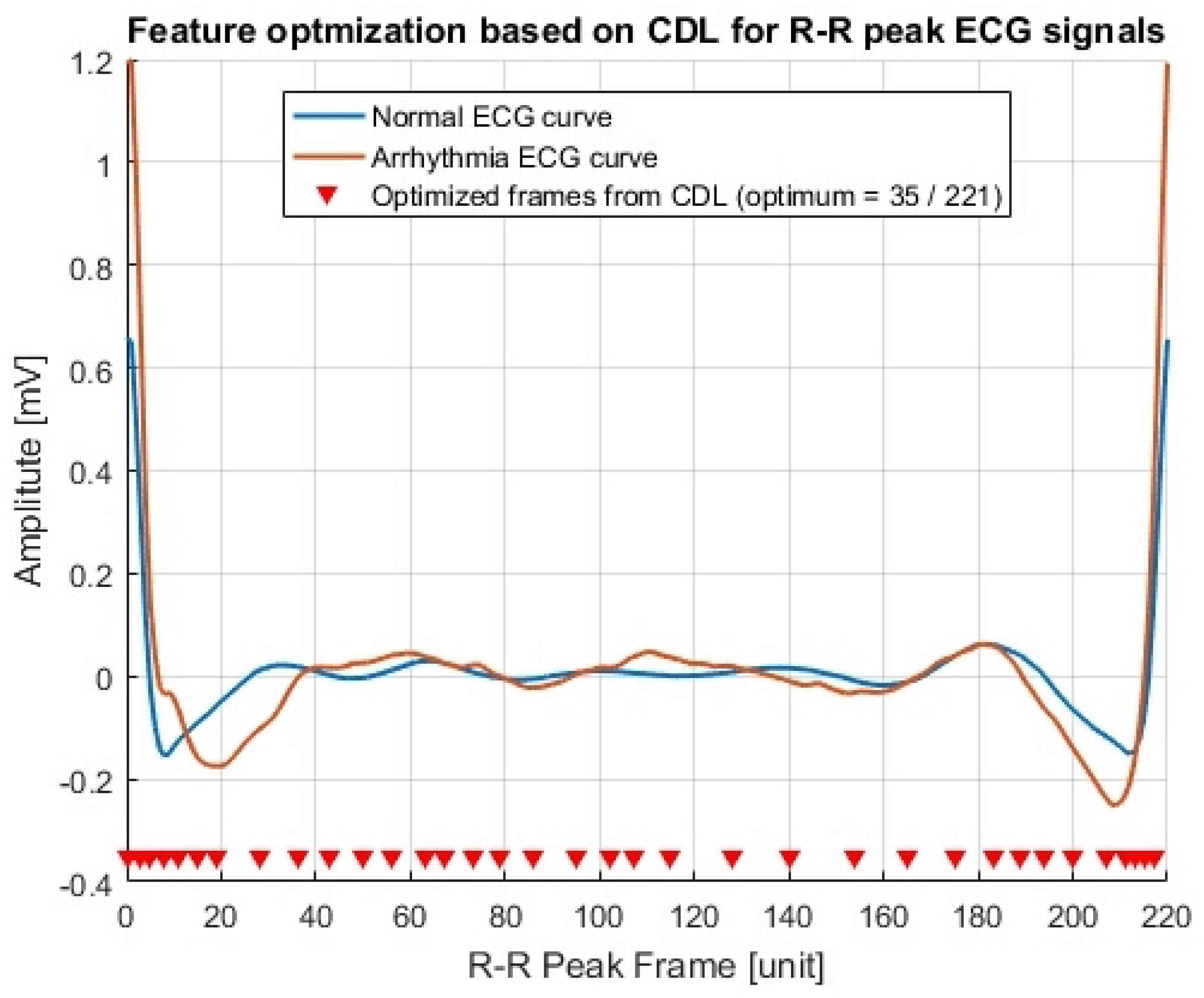
where is the accuracy of the original ML system which has the input feature. According to various trials of machine learning training, gives enough resemblance compared to an original input feature although an optimal correlation threshold might be arbitrarily chosen. The CDL for optimizing the input features of the compact arrhythmia detection system [33] has been visualized on Figure 1 with a threshold for the input feature of (i.e., ). Although a preselected value might not be the best solution for reducing the input feature of an ML system, it could provide faster training time than the original training time because the number of input features has been reduced.
Figure 1 displays several original sliced ECG samples obtained using the RRIF (RR-interval-framed) technique [23,33]. Each value on the sliced ECG signal serves as an input feature, resulting in a total of 220 input features for ML training. As demonstrated in the figure, the implementation of the CDL approach effectively reduces the feature count to 36 [33].
2.2. Reducing Samples of Machine Learning Systems
The main idea of finding the number of samples is that the probability distributions of the subsets A and B have the same probability distribution as the population , although the sample sizes of the subsets are smaller than the sample size of the population. Let X be an input data point which is the random variable based on the samples in a subset, and the probability of a hypothesis test is defined as follows:
where is a small number which is a tolerance of samples and is the target probability for a resemblance between the population mean and a sample mean with the standard deviation of the population . The minimum number of samples for each feature k is as follows:
where (the standard normal distribution)
and
which could be calculated from the population which contains samples. Let be the set of output classes (i.e., types of the output). Each original sample (or trial) is mapped with one of these classes within , and is the number of class outputs. Let be the (mother) set of the required sample sizes for the output class r as follows from (9):
and
where is the samples of the input feature k given the output class r, and is the number of samples which are labeled with the output class r. The average number of samples for each input feature is as follows:
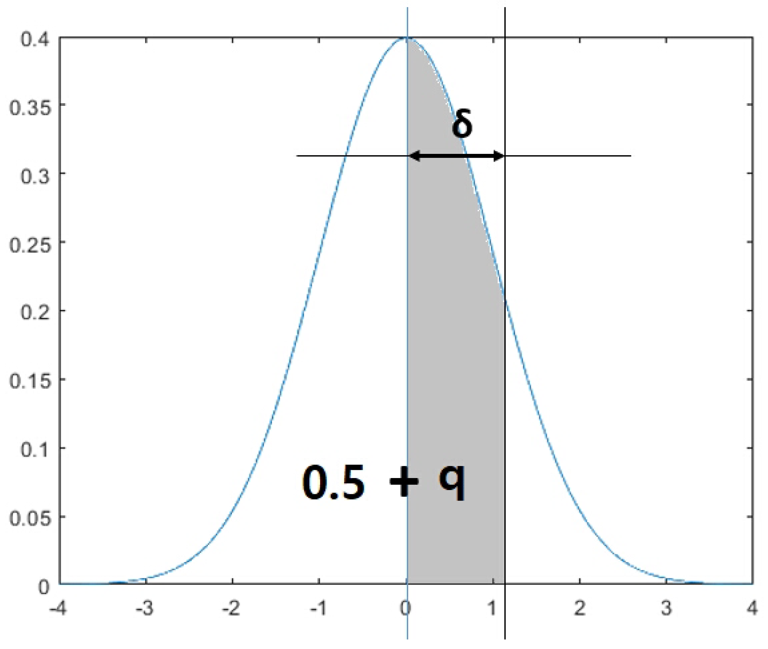
which could be chosen as the optimal sample size for the ML training dataset. It is noted that is a tolerance range which indicates how far the sample size is from the mean of the standard normal distribution (see Figure 2). The function gives the z-value which indicates adding probability q after passing the mean of the standard normal distribution (i.e., ).
3. Case Study: Compact Arrhythmia Detection
This section demonstrates compact data learning for ML training. A deep learning model for the detection of arrhythmia was developed in which time-sliced ECG data representing the distance between successive R-peaks were used as the input for a convolutional neural network [23,33]. CDL could optimize the input dataset by reducing both input features and sample size. The performance for each case is fully explained in this section.
3.1. Experiment Setups
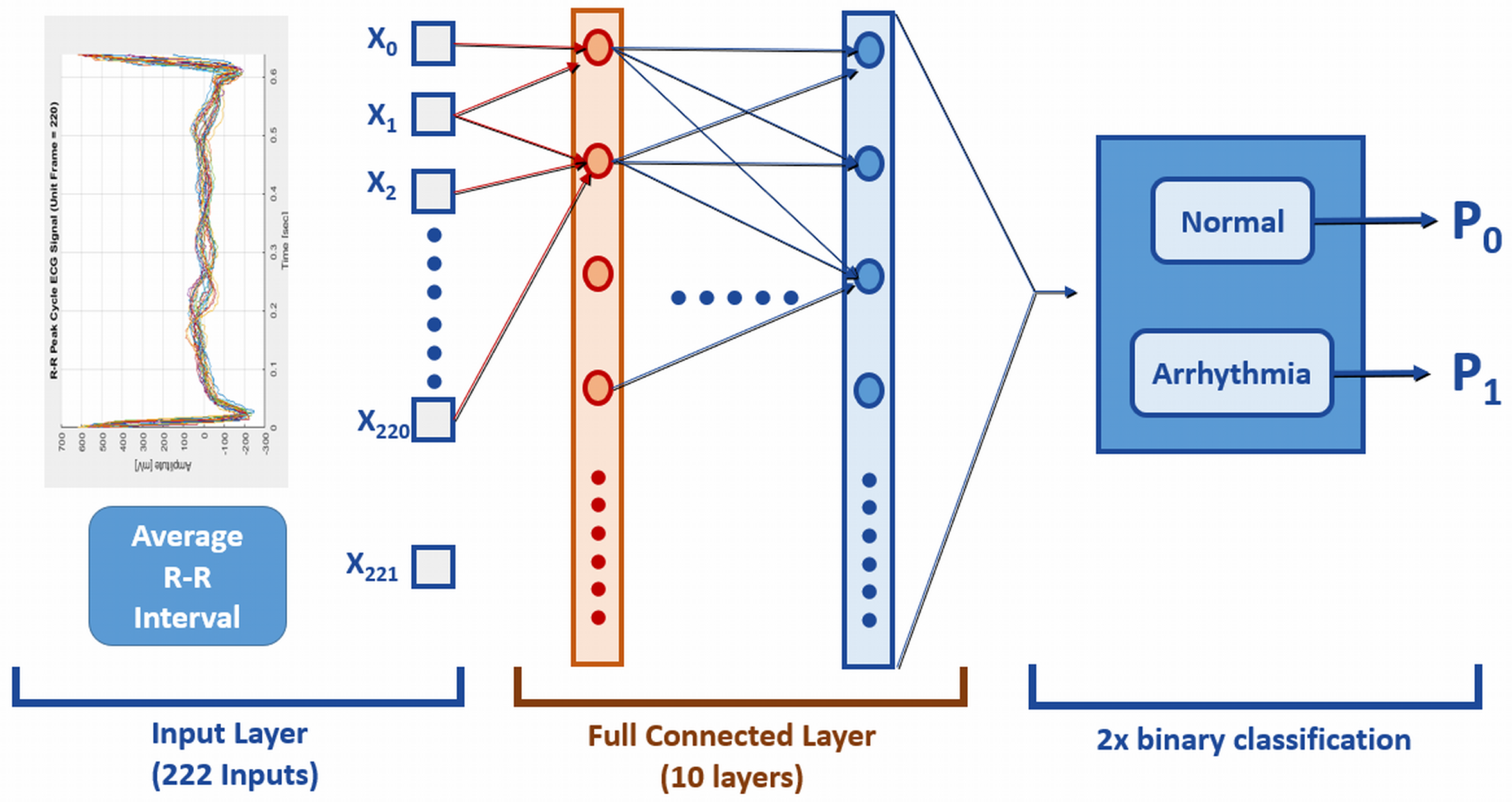
The original ECG dataset, obtained from PhysioNet [33,37], consists of 1019 sliced ECG samples and 222 input features. The dataset is labeled with a binary classification (0—normal, 1—arrhythmia). A separate set of samples is designated as the training dataset for comparing different ML system variants. The testing dataset, containing 1085 samples, shares the same 222 input features and the single binary output as the training dataset, but with no overlap. As the reference ML system for training, a 10-layered CNN was employed to evaluate the efficiency of compact data. The CNN architecture for arrhythmia detection is depicted in Figure 3. In this particular case study, the ML system comprised 222 input features, a single binary output, and 10 hidden layers [33].
According to previous research [33], the accuracy of the arrhythmia detection using the original training dataset (refer to Table 1) reached accuracy. This evaluation was conducted on 1085 testing samples. It is important to note that each training session, even with the same original dataset, may yield varying accuracies due to the specific properties associated with CNN machine learning training.
Hence, a hypothesis test comparing our model with the original dataset was necessary to evaluate the ML accuracy post-CDL adaptation. It is noted that the optimization of ML algorithms falls outside the purview of this research, and a reference system is required to evaluate the optimization of input features and training samples.
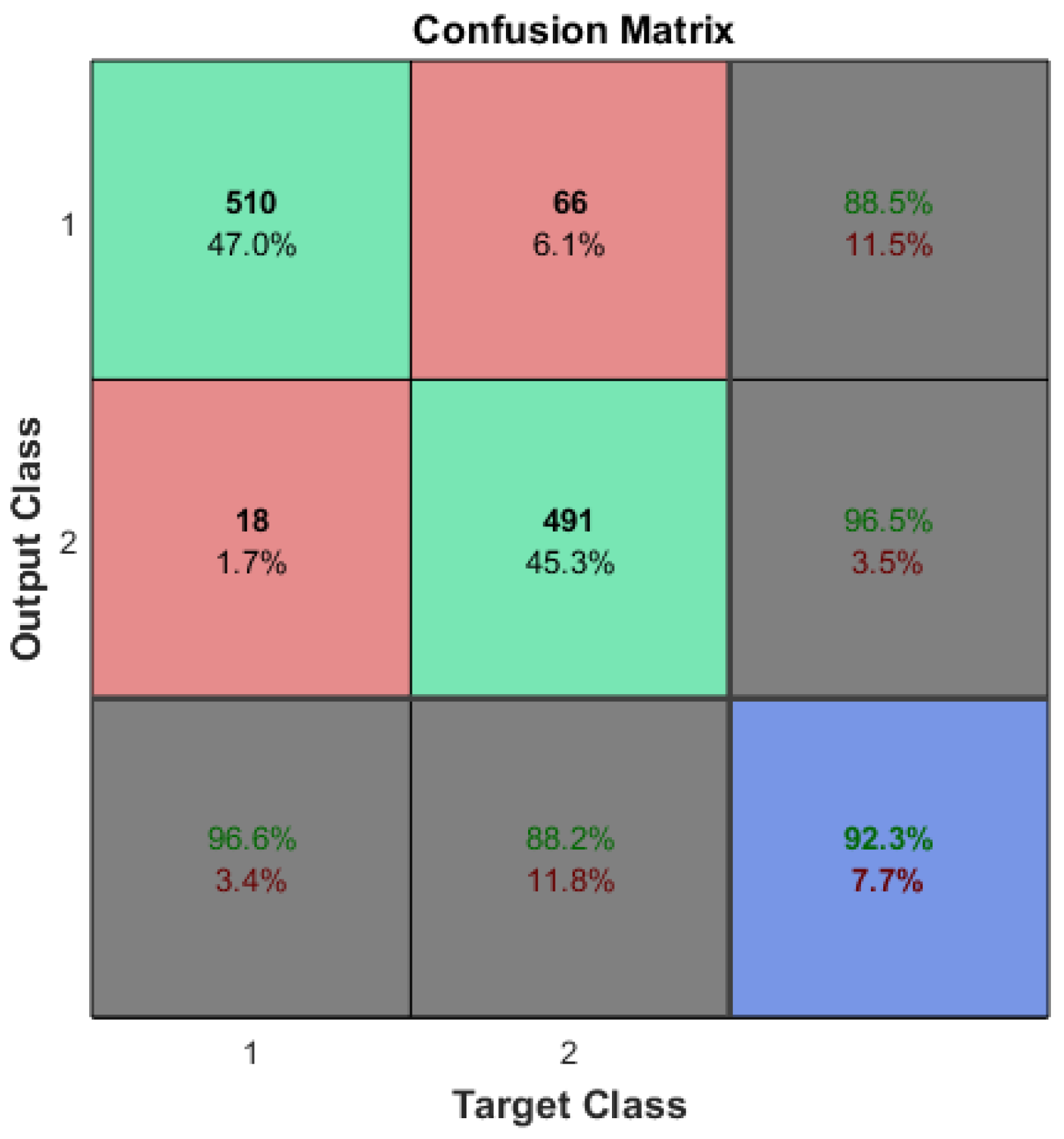
The optimization of ML algorithms could be a subject for future research. The accuracies of machine learning systems should be statistically identical even with the application of CDL. In the case of arrhythmia detection, a reference accuracy of approximately 92% (see Figure 4) is desired, even after the reduction in input features and/or sample sizes.
3.2. Reduced Input Features
The theoretical methodology presented in the previous section for reducing input features was implemented in the ML training for arrhythmia detection. As mentioned, the default hyper-parameter for the correlation, , was set to . It is important to note that while the optimal value of the correlation threshold depends on the training data, the default value of is considered reasonable as a hyper-parameter (refer to Figure 1). If , the input features in each pair are classified as strongly correlated, and one of them is selected for removal. Based on Equations (3)–(5), the original input feature set and the optimized input feature set are determined as follows:
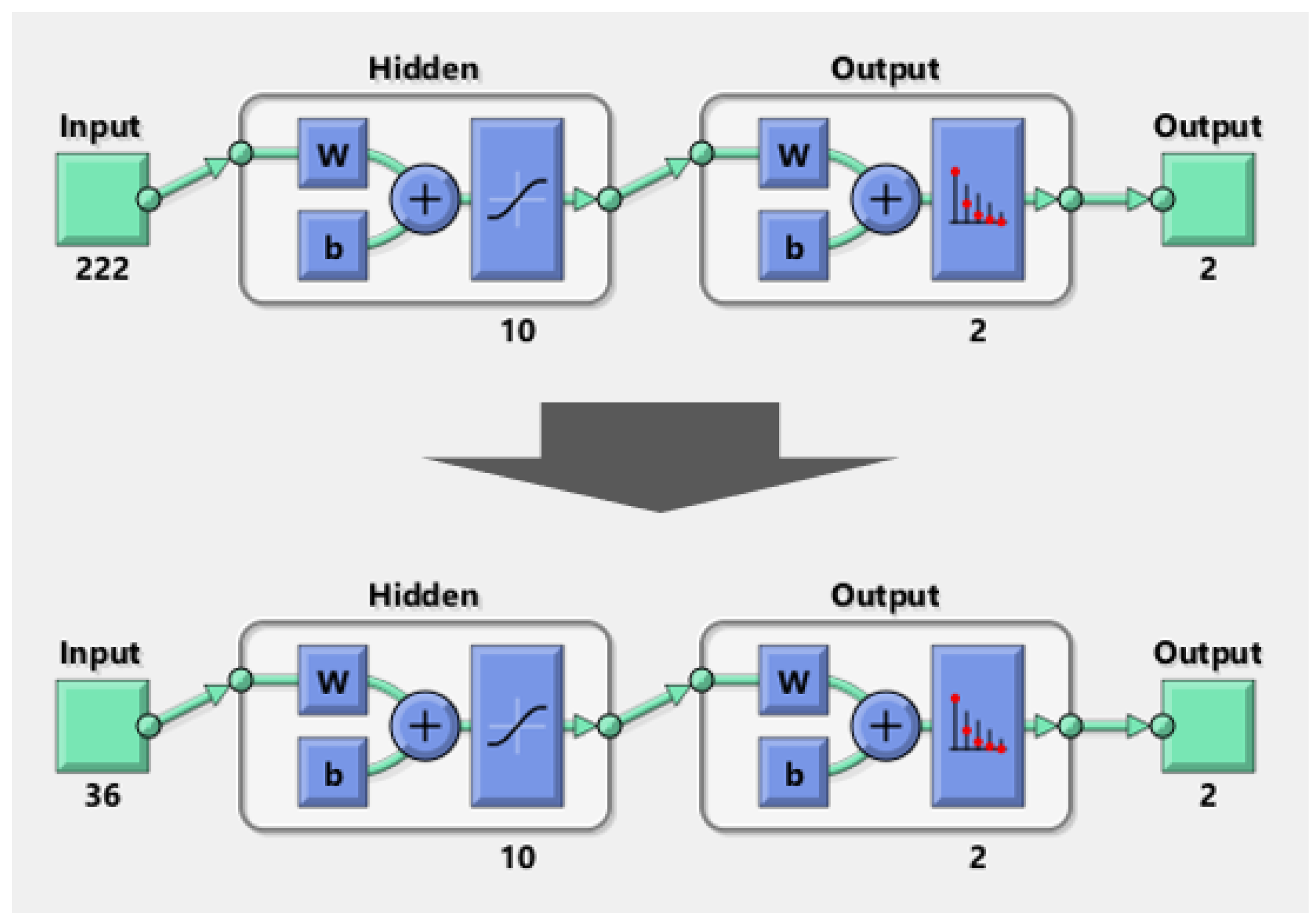
After adapting the CDL, the total number of input features was reduced to . Since the input features were reduced to 36 from 222, the CNN model was redesigned accordingly (see Figure 5).
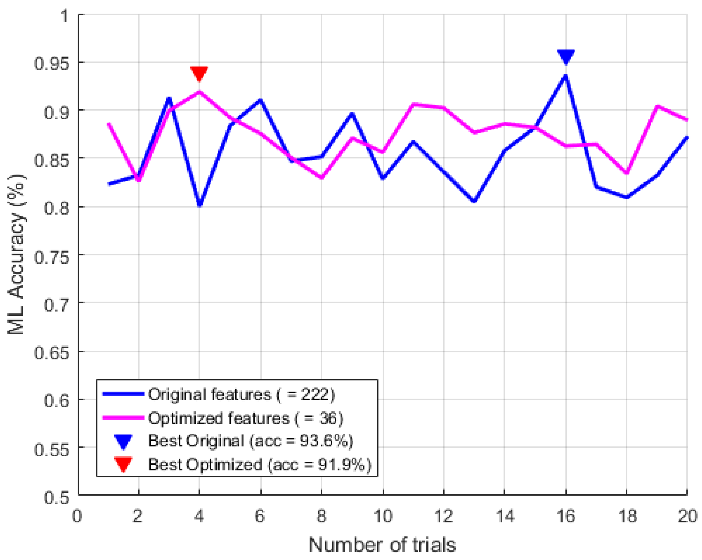
The optimized input feature set may not be identical even with the same correlation threshold, as it depends not only on the correlation but also on the training dataset itself. As stated in the previous section, the accuracy based on the initial training dataset was from Equation (12) (i.e., ), and the accuracy after reducing the input features was (i.e., ) as seen in Figure 6. While the accuracy after input feature reduction (i.e., ) was statistically the same as the accuracy with the original input features (i.e., ) on the original training dataset, it is possible that machine learning training with optimized input features may yield improved performance at times.
The t-test was applied to check whether the means of the accuracy of these two cases (i.e., , ) were statistically the same or not. The most common application of the t-test is to test whether the means of two populations are different.
As shown in Figure 7, the accuracy of the compact arrhythmia detection by using CDL was statistically the same as with the original number of input features because the null hypothesis was accepted based on 20 trials (i.e., ).
3.3. Reduced Sample Size
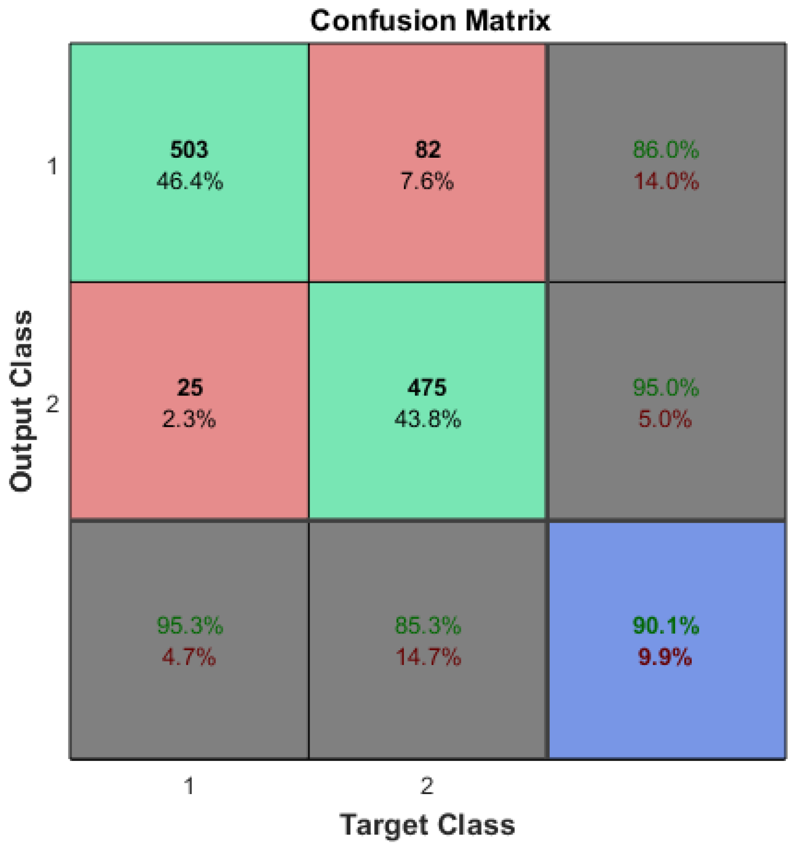
The theoretical methodology for reducing the sample size in the previous section was applied to the compact arrhythmia detection ML training. The hyper-parameter q for the sample reduction was determined as (i.e., ). From (8)–(9) and (15), the samples were reduced to 836 from the original sample size (i.e., = 1019 in Table 1). As can be seen in Figure 8, the accuracy after reducing samples did not change even after optimizing samples. From (4), the reduced samples are shown in Figure 8.
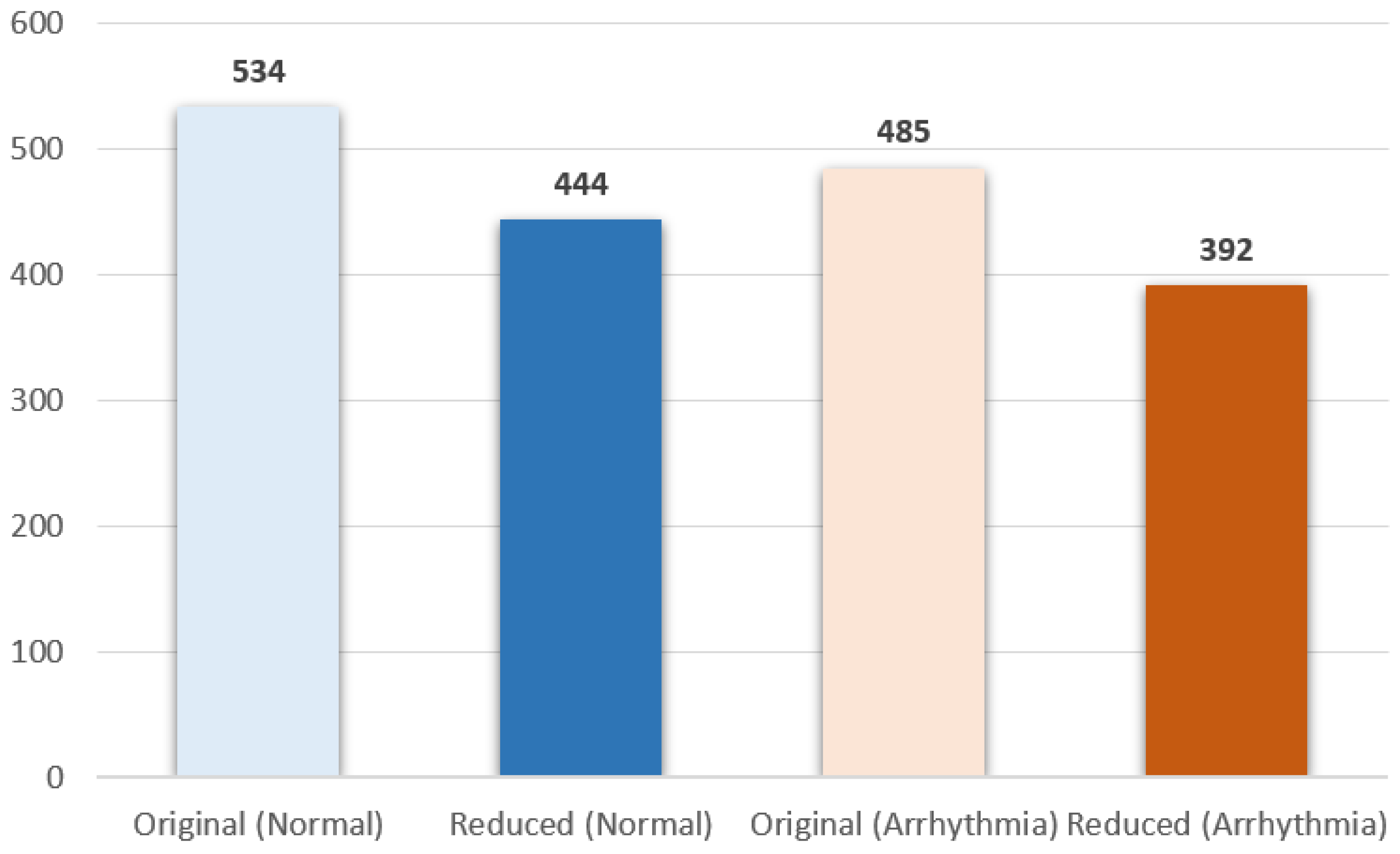
The number of normal and arrhythmia samples was 534 and 485, respectively, (see Figure 9), and the sample size was reduced by , which means the total number of training samples became 836 from 1019 during the training.
It is noted that the number of input features was not revised (i.e., in Table 1). The Figure 10 shows that the accuracy of the compact arrhythmia detection when using CDL was statistically the same as with the original number of the training samples because the null hypothesis was accepted based on 20 trials.
3.4. Overall Performance
The previous subsections in Section 3 showed that the accuracy of the ML system did not change even after optimizing the training dataset. The accuracy after reducing both input features and samples were also statistically the same (see Figure 11).
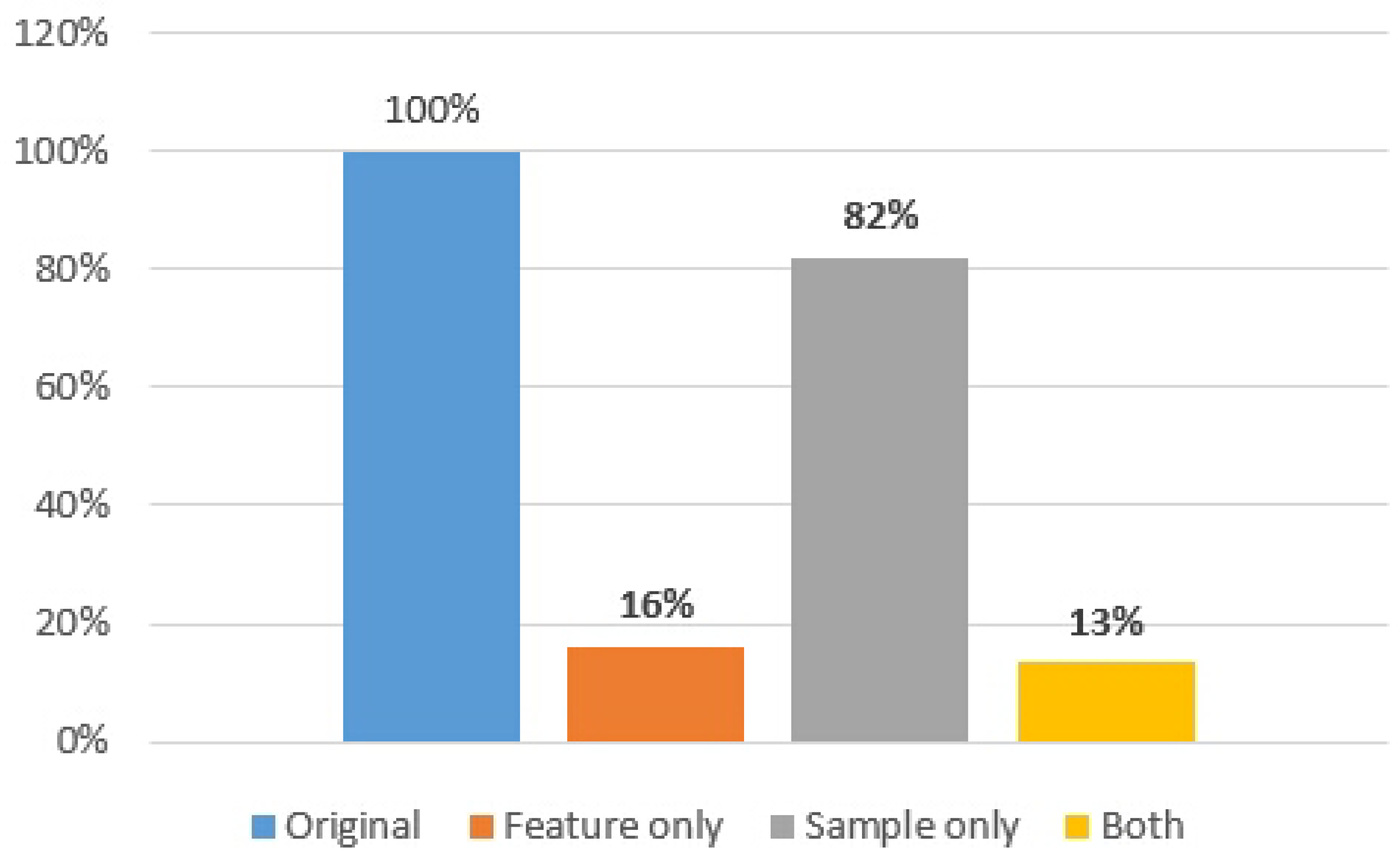
The ML training data size was significantly diminished due to the application of CDL. By reducing the input features, the original data size was trimmed down to 16% of the initial dataset. When the sample size was reduced, it dropped to 82%. When both optimizations of CDL were implemented, the training data size could be curtailed to as low as 13% (refer to Figure 12).
The application of the CDL method for machine learning (ML) training proved to be remarkably efficient. Despite utilizing only about one-seventh of the original training data size, it maintained statistical parity with the accuracy of the original arrhythmia detection mechanism. This implies that the CDL-optimized model, while being far more resource-efficient, does not compromise the quality of the results. It is a testament to the potential of CDL in improving the efficiency of ML training, particularly in scenarios where data size might pose a challenge. By reducing the data size without affecting the accuracy, CDL presents a promising advancement in the field of ML training for arrhythmia detection.
4. Challenges and Future Research
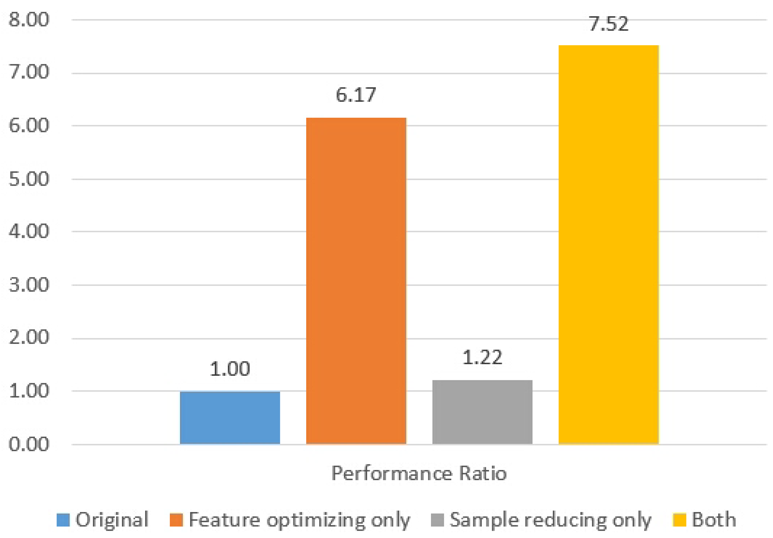
Digesting the huge size of training dataset for ML systems has been a vital issue to achieve a breakthrough in traditional systems. However, current mechanisms require one or several additional ML training rounds before optimizing an ML model. Compact data learning, which uses basic statistical methods including correlation and hypothesis tests has been newly proposed. This method could optimize an ML training dataset without additional training sessions. A total of 1019 arrhythmia samples with 222 input features were trained as the reference, and various CDL techniques were constructed with the same statistical accuracy. This research found that the ML training dataset could be minimized by reducing the input features to 36 and the number of samples to 836, which corresponds to a reduction of more than seven times compared to the original model while maintaining the same statistical accuracy performance (i.e., in Figure 13).
While this research has laid the foundation for compact data learning (CDL), there remain some challenges that warrant further investigation. The primary challenges of CDL include (1) its applicability being limited to classification problems; (2) the complexity involved in calculating pairwise correlations; and (3) the optimization of the correlation threshold. Recommendations on how to address these challenges are provided in the following subsections, concluding this paper.
4.1. The Complexity of Correlation Calculation
The calculation of correlation in statistics is relatively simple, but computing pairwise correlations requires significant computational power, potentially exceeding that required for machine learning training. Pairwise correlation involves calculating all correlations between pairs of input features in a training dataset. Explainable AI (XAI) could serve as an alternative solution for optimizing the number of input features if the computation of pairwise correlations is slower than machine learning training. XAI aims to develop a range of techniques that generate more explainable models while maintaining high performance levels [11,12]. However, it necessitates an additional round of ML training solely for optimizing the input features. While it has been assumed that calculating correlations within the training dataset is superior to ML training for XAI, this statement has not been fully validated. Validating the complexity of pairwise correlations compared to ML model training could be a potential area for future research. Alternatively, users may be more interested in providing the appropriate indicator (e.g., cost function) to determine when CDL (i.e., calculating correlations to reduce input features) is more suitable than XAI (i.e., additional ML model training to evaluate input features).
4.2. The Correlation Threshold Optimization
In Section 2, the correlation threshold was arbitrarily determined based on the practice in the industry, but finding the optimal threshold for reducing the number of input features could be another research topic to improve CDL. The correlation threshold is formally described as follows:
where is the null hypothesis for the two-sample Z-test, and the revised set of the input features is from (5). The elements of the set are collected from the medium set of correlation pairs from (4). The threshold for cutting input features can be found by using the two-sample Z-test, and the test statistic is as follows:
where u is the number of trials for ML training. Since multiple machine learning training sessions may generate different simulation results due to different initial conditions and folding samples, a certain number of trials are required to get the statistical confidence. From (5) and (19), the test statistic can be the function based on a correlation as follows:
From (6) and (20), the threshold of input features is formulated as follows:
where is the confidence level of the Z-test. The inverse of the CDF is an inverse function of the standard normal distribution (9). It is noted that the threshold for cutting input features based on a correlation depends on the training data samples and the accuracy of the ML system. Therefore, an optimum cannot be found until massive trials are completed. Additionally, the minimum threshold might be overfitting a trained machine learning system. That is one of the reasons why should be preselected as a hyper-parameter (see Section 2). The primary goal of CDL is to maintain a similar machine learning accuracy while speeding up ML training. However, simply increasing accuracy by reducing the training dataset can sometimes lead to overfitting, particularly if the number of input features is too small. Overfitting occurs when a model becomes too attuned to the training data and performs poorly with new data. Therefore, while CDL aims to expedite ML training and maintain accuracy, it is crucial to ensure the model robustness and its ability to generalize to new data to avoid overfitting. As CDL is designed for simplicity and broad applicability, the CDL framework in this study did not encompass specific hyper-parameters, such as the correlation threshold for the input feature selection and delta for determining optimal sample sizes. However, these specific factors can be addressed using a tailor-made compact data approach aimed at stabilizing particular ML algorithms or optimizing ML-based systems by adapting various methods targeting a specific ML algorithm or a specific data-driven system. Designing tailor-made compact data for a particular system remains an active area of future research.
5. Conclusions
This research presented an innovative approach for enhancing machine learning training, introducing a framework known as compact data learning (CDL). Designed to accelerate the training phase without sacrificing system accuracy, this novel framework provides unique and groundbreaking strategies for creating compact data in a wider context. Upon the experiments, the data size of ML training was dramatically reduced by using compact data learning. The original data size was reduced by 16% for the input features and 82% for the sample size. When both optimizations were applied, the training data size was reduced by up to 13% of the original dataset. CDL serves as a guide for adopting this cutting-edge method to boost model training efficiency. Despite the existence of numerous challenges that remain to be addressed in future research, this framework holds promise for application across various domains, including ML-based ECG biometric authentication, credit card fraud detection, and malware detection systems.
Funding
This work was supported in part by the Macao Polytechnic University (MPU), under grant RP/FCA-04/2023.
Data Availability Statement
Data is contained within the article.
Acknowledgments
This paper was revised using AI/ML-assisted tools. Special thanks to the reviewers who provided valuable advice for improving this paper.
Conflicts of Interest
The author declares no conflict of interest.
References
- Barreno, M.A.; Nelson, B.A.; Sears, R.; Joseph, A.D.; Tygar, J.D. Can machine learning be secure? In Proceedings of the 2006 ACM Symposium on Information, Computer and Communications Security, Taipei, Taiwan, 21–24 March 2006; pp. 16–25. [Google Scholar]
- Xu, Z.; Saleh, J.H. Machine learning for reliability engineering and safety applications: Review of current status and future opportunities. arXiv 2021, arXiv:2008.08221. [Google Scholar] [CrossRef]
- Drira, K.; Wang, H.; Yu, Q.; Wang, Y.; Yan, Y.; Charoy, F.; Mendling, J.; Mohamed, M.; Wang, Z.; Bhiri, S. Data provenance model for internet of things (iot) systems. In Proceedings of the Service-Oriented Computing—ICSOC 2016 Workshops, Banff, AB, Canada, 10–13 October 2016; pp. 85–91. [Google Scholar]
- Russell, S.J.; Norvig, P. Artificial Intelligence: A Modern Approach, 3rd ed.; Prentice Hall: Englewood Cliffs, NJ, USA, 2010. [Google Scholar]
- Mohri, M.; Rostamizadeh, A.; Talwalkar, A. Foundations of Machine Learning; The MIT Press: Cambridge, MA, USA, 2012. [Google Scholar]
- Ramirez, M.A.; Kim, S.-K.; Hamadi, H.A.; Damiani, E.; Byon, Y.-J.; Kim, T.-Y.; Cho, C.-S.; Yeun, C.Y. Poisoning Attacks and Defenses on Artificial Intelligence: A Survey. arXiv 2022, arXiv:2202.10276. [Google Scholar]
- Wang, Y.; Yao, Q.; Kwok, J.; Ni, L.M. Generalizing from a Few Examples: A Survey on Few-Shot Learning. arXiv 2019, arXiv:1904.05046. [Google Scholar] [CrossRef]
- Fei-Fei, L.; Fergus, R.; Perona, P. One-shot learning of object categories. IEEE Trans. Pattern Anal. Mach. Intell. 2006, 28, 594–611. [Google Scholar] [CrossRef]
- Fink, M. Object classification from a single example utilizing class relevance metrics. In Proceedings of the 17th International Conference on Neural Information Processing Systems, NIPS 2004, Vancouver, BC, Canada, 13–18 December 2004; pp. 449–456. Available online: https://www.researchgate.net/publication/221619654_Object_Classification_from_a_Single_Example_Utilizing_Class_Relevance_Metrics (accessed on 10 January 2024).
- Shu, J.; Xu, Z.; Meng, D. Small sample learning in big data era. arXiv 2018, arXiv:1808.04572. [Google Scholar]
- Adadi, A.; Berrada, M. Peeking Inside the Black-Box: A Survey on Explainable Artificial Intelligence (XAI). IEEE Access 2018, 6, 52138–52160. [Google Scholar] [CrossRef]
- Tjoa, E.; Guan, C. A Survey on Explainable Artificial Intelligence (XAI): Toward Medical XAI. IEEE Trans. Neural Netw. Learn. Syst. 2021, 32, 4793–4813. [Google Scholar] [CrossRef]
- Fisher, A.; Rudin, C.; Dominici, F. Model class reliance: Variable importance measures for any machine learning model class. arXiv 2018, arXiv:1801.01489. [Google Scholar]
- Casalicchio, G.; Molnar, C.; Bischl, B. Visualizing the feature importance for black box models. arXiv 2018, arXiv:1804.06620. [Google Scholar]
- Lei, J.; G’Sell, M.; Rinaldo, A.; Tibshirani, R.J.; Wasserman, L. Distribution-free predictive inference for regression. J. Am. Stat. Assoc. 2018, 113, 1094–1111. [Google Scholar] [CrossRef]
- Al-Hammadi, A.Y.; Yeun, C.Y.; Damiani, E.; Yoo, P.D.; Hu, J.; Yeun, H.K.; Yim, M.-S. Explainable artificial intelligence to evaluate industrial internal security using EEG signals in IoT framework. Ad Hoc Netw. 2020, 123, 102641. [Google Scholar] [CrossRef]
- Kim, S.K. Toward Compact Data from Big Data. In Proceedings of the 2020 15th International Conference for Internet Technology and Secured Transactions (ICITST), London, UK, 8–10 December 2020; pp. 1–5. [Google Scholar]
- Dean, J. Big Data, Data Mining, and Machine Learning; Wiley: Hoboken, NJ, USA, 2014. [Google Scholar]
- Battams, K. Stream processing for solar physics: Applications and implications for big solar data. arXiv 2020, arXiv:1409.8166. [Google Scholar]
- Kambatla, K.; Kollias, G.; Kumar, V.; Grama, A. Trends in big data analytics. J. Parallel. Distrib. Comput. 2014, 74, 2561–2573. [Google Scholar] [CrossRef]
- Kim, S.K.; Yeun, C.Y.; Damiani, E.; Lo, N.-W. A Machine Learning Framework for Biometric Authentication using Electrocardiogram. IEEE Access 2019, 7, 94858–94868. [Google Scholar] [CrossRef]
- Al Alkeem, E.; Kim, S.K.; Yeun, C.Y.; Zemerly, M.J.; Poon, K.F.; Gianini, G.; Yoo, P.D. An Enhanced Electrocardiogram Biometric Authentication System Using Machine Learning. IEEE Access 2019, 7, 123069–123075. [Google Scholar] [CrossRef]
- Kim, S.K.; Yeun, C.Y.; Yoo, P.D. An Enhanced Machine Learning-based Biometric Authentication System Using RR-Interval Framed Electrocardiograms. IEEE Access 2019, 7, 168669–168674. [Google Scholar] [CrossRef]
- Yoon, S.; Cantwell, W.J.; Yeun, C.Y.; Cho, C.S.; Byon, Y.J.; Kim, T.Y. Defect Detection in Composites by Deep Learning using Highly Nonlinear Solitary Waves. Int. J. Mech. Sci. 2023, 239, 107882. [Google Scholar] [CrossRef]
- Akogul, S. A Novel Approach to Increase the Efficiency of Filter-Based Feature Selection Methods in High-Dimensional Datasets with Strong Correlation Structure. IEEE Access 2023, 11, 115025–115032. [Google Scholar] [CrossRef]
- Chandrashekar, G.; Sahin, F. A survey on feature selection methods. Comput. Electr. Eng. 2014, 40, 16–28. [Google Scholar] [CrossRef]
- Chuang, L.-Y.; Chang, H.-W.; Tu, C.-J.; Yang, C.-H. Improved binary PSO for feature selection using gene expression data. Comput. Biol. Chem. 2008, 32, 29–38. [Google Scholar] [CrossRef]
- Peng, H.; Long, F.; Ding, C. Feature selection based on mutual information criteria of max-dependency, max-relevance, and min-redundancy. IEEE Trans. Pattern Anal. Mach. Intell. 2005, 27, 1226–1238. [Google Scholar] [CrossRef] [PubMed]
- Jaeger, J.; Sengupta, R.; Ruzzo, W.L. Improved Gene Selection for Classification of Microarrays. Proc. Pac. Symp. Biocomput. 2003, 53–64. [Google Scholar] [CrossRef]
- Jain, A.K.; Duin, R.P.W.; Mao, J. Statistical Pattern Recognition: A Review. IEEE Trans. Pattern Anal. Mach. Intell. 2000, 22, 4–37. [Google Scholar] [CrossRef]
- Kwak, N.; Choi, C.H. Input Feature Selection by Mutual Information Based on Parzen Window. IEEE Trans. Pattern Anal. Mach. Intell. 2002, 24, 1667–1671. [Google Scholar] [CrossRef]
- Iannarilli, F.J.; Rubin, P.A. Feature Selection for Multiclass Discrimination via Mixed-Integer Linear Programming. IEEE Trans. Pattern Anal. Mach. Intell. 2003, 25, 779–783. [Google Scholar] [CrossRef]
- Kim, S.-K.; Yeun, C.Y.; Yoo, P.D.; Lo, N.-W.; Damiani, E. Deep Learning-Based Arrhythmia Detection Using RR-Interval Framed Electrocardiograms. In Proceedings of the Eighth International Congress on Information and Communication Technology, London, UK, 20–23 February 2023; pp. 11–21. [Google Scholar]
- Ross, S. A First Course in Probability, 8th ed.; Prentice Hall: Upper Saddle River, NJ, USA, 2010. [Google Scholar]
- Kosorok, M.R. On Brownian Distance Covariance and High Dimensional Data. Ann. Appl. Stat. 2009, 3, 1266–1269. [Google Scholar] [CrossRef] [PubMed]
- Székely, G.J.; Rizzo, M.L.; Bakirov, N.K. Measuring and testing dependence by correlation of distances. Ann. Stat. 2007, 35, 2769–2794. [Google Scholar] [CrossRef]
- Goldberger, A.L.; Amaral, L.A.; Glass, L.; Hausdorff, J.M.; Ivanov, P.C.; Mark, R.G.; Mietus, J.E.; Moody, G.B.; Peng, C.K.; Stanley, H.E. PhysioBank Physio Toolkit, and PhysioNet: Components of a New Research Resource for Complex Physiologic Signals. Circulation 2000, 101, e215–e220. [Google Scholar] [CrossRef]
Figure 1.
Optimizing the input features for ECG based arrhythmia detection ().

Figure 2.
Calculating the tolerance range of samples sizes for each feature based on the normal distribution.
Figure 2.
Calculating the tolerance range of samples sizes for each feature based on the normal distribution.

Figure 3.
Reference CNN model for the arrhythmia detection [33].
Figure 3.
Reference CNN model for the arrhythmia detection [33].

Figure 4.
The confusion matrix of the arrhythmia detection which was trained on the original dataset.
Figure 4.
The confusion matrix of the arrhythmia detection which was trained on the original dataset.

Figure 5.
The CNN model for arrhythmia detection after optimizing the input features (i.e., ).

Figure 6.
Compact arrhythmia detection confusion matrix after optimizing the number of input features.
Figure 6.
Compact arrhythmia detection confusion matrix after optimizing the number of input features.

Figure 7.
The t-test of two compact arrhythmia detection cases for optimizing the input features ().
Figure 7.
The t-test of two compact arrhythmia detection cases for optimizing the input features ().

Figure 8.
Compact arrhythmia detection confusion matrix after reducing the sample size.

Figure 9.
Optimized number of training samples.

Figure 10.
The t-test of two compact arrhythmia detection cases for optimizing the number of samples ().
Figure 10.
The t-test of two compact arrhythmia detection cases for optimizing the number of samples ().

Figure 11.
Arrhythmia detection confusion matrix when using CDL for optimizing the features and the samples together.
Figure 11.
Arrhythmia detection confusion matrix when using CDL for optimizing the features and the samples together.

Figure 12.
Data size comparison when using CDL for the arrhythmia detection.

Figure 13.
Performance comparison for the arrhythmia detection.


Table 1.
The CDL experiment setup with the compact arrhythmia detection dataset [33].
Table 1.
The CDL experiment setup with the compact arrhythmia detection dataset [33].
| Parameter | Setup Value | Description |
|---|---|---|
| m | 222 | Total number of initial input features |
| 1019 | Total number of initial training samples | |
| 2 | Number of output classes | |
| 0.8 | Correlation threshold | |
| 0.8416 | Tolerance range |
Disclaimer/Publisher’s Note: The statements, opinions and data contained in all publications are solely those of the individual author(s) and contributor(s) and not of MDPI and/or the editor(s). MDPI and/or the editor(s) disclaim responsibility for any injury to people or property resulting from any ideas, methods, instructions or products referred to in the content. |
© 2024 by the author. Licensee MDPI, Basel, Switzerland. This article is an open access article distributed under the terms and conditions of the Creative Commons Attribution (CC BY) license (https://creativecommons.org/licenses/by/4.0/).
Share and Cite
MDPI and ACS Style
Kim, S.-K. Compact Data Learning for Machine Learning Classifications. Axioms 2024, 13, 137. https://doi.org/10.3390/axioms13030137
AMA Style
Kim S-K. Compact Data Learning for Machine Learning Classifications. Axioms. 2024; 13(3):137. https://doi.org/10.3390/axioms13030137
Chicago/Turabian StyleKim, Song-Kyoo (Amang). 2024. "Compact Data Learning for Machine Learning Classifications" Axioms 13, no. 3: 137. https://doi.org/10.3390/axioms13030137
Note that from the first issue of 2016, this journal uses article numbers instead of page numbers. See further details here.