


Asymptotic Representation of Vorticity and Dissipation Energy in the Flux Problem for the Navier–Stokes Equations in Curved Pipes

1
Department of Mathematics and Mechanics, Novosibirsk State University, Pirogova Str. 2, Novosibirsk 630090, Russia
2
Lavrentyev Institute of Hydrodynamics SB RAS, Lavrentyev Pr. 15, Novosibirsk 630090, Russia
3
Basic Studies Department, Siberian State University of Telecommunications and Information Science, Kirova Str. 86, Novosibirsk 630102, Russia
*
Author to whom correspondence should be addressed.
†
These authors contributed equally to this work.
Axioms 2024, 13(1), 65; https://doi.org/10.3390/axioms13010065
Submission received: 1 December 2023
/
Revised: 11 January 2024
/
Accepted: 16 January 2024
/
Published: 19 January 2024
(This article belongs to the Special Issue Fluid Dynamics: Mathematics and Numerical Experiment)
Abstract
:This study explores the problem of describing viscous fluid motion for Navier–Stokes equations in curved channels, which is important in applications like hemodynamics and pipeline transport. Channel curvature leads to vortex flows and closed vortex zones. Asymptotic models of the flux problem are useful for describing viscous fluid motion in long pipes, thus considering geometric parameters like pipe diameter and characteristic length. This study provides a representation for the vorticity vector and energy dissipation in the flow problem for a curved channel, thereby determining the magnitude of vorticity and energy dissipation depending on the channel’s central line curvature and torsion. The accuracy of the asymptotic formulas are estimated in terms of small parameter powers. Numerical calculations for helical tubes demonstrate the effectiveness of the asymptotic formulas.
1. Introduction
The description of viscous fluid motion in a curved channel is a complex problem in theoretical hydrodynamics [1] and has significant relevance in various applications, such as hemodynamics [2,3,4] and pipeline transport [5]. Channel curvature leads to a rearrangement of flow topology, the formation of vortex flows, and closed vortex zones. To date, the only parameter determining the influence of weak channel curvature on the nature of slow flow remains the Dean number [6]. This parameter is not universal and does not define the complete map of flow regimes, particularly the appearance of vortex zones in channels with different geometries. From a mathematical perspective, this is due to the complexity of the Navier–Stokes equations when working with a curved channel [7,8,9], and the boundary conditions can be formulated in terms of the vortex [10]. In this situation, asymptotic models of flow problems are useful, thus describing the motion of viscous fluid in long pipes. In this case, the small parameter is the ratio of the pipe diameter to its characteristic length. For straight and long pipes with branching nodes, a developed asymptotic theory exists [11], which has effective applications in mathematical medicine [4]. For curved pipes, the consideration of geometric parameters becomes important. Works such as [12,13,14] have developed asymptotic theories of flow problems, thereby taking into account the channel geometry through the curvature and torsion of the central axis of the tube. These works provide asymptotic representations of the main flow parameters (velocity and pressure) for both steady and unsteady motion and for different behaviors of the channel walls (rigid or elastic). In fluid dynamics, the resistance force and the energy required for fluid propulsion are significant [6,8]. For a viscous fluid, the resistance force is computed through the energy dissipation, which is represented by an integral over the flow region of the square of the vorticity vector modulus [15,16,17,18].
In this study, using asymptotic theory, we provide a representation for the vorticity vector in a curved tube in terms of small parameter powers. The aim of the paper is to derive, on the basis of the paper [14], asymptotic formulas for the vorticity and drag, as well as the dissipation energy of the flow in the flow problem for the Navier–Stokes equations in a curved pipe. These formulas give uniform estimates of the deviation of the solution from the exact one by a small parameter characterizing the pipe length. In these formulas, with the following being very important, the influence of characteristic parameters (the curvature and torsion of the pipe center line on the flow geometry) is explicitly taken into account. The asymptotic representation of the solution allows us to explicitly separate within it the components that depend on the geometry and the part that does not depend on it. The latter is determined by the solution of the standard problems (3)–(5) in the pipe cross-section. This representation is important for determining the influence on the flow of both the cross-section and the pipe curvature, which determines the intensity of vortex formation. The value of the dissipation energy allows us to calculate the additional work that must be expended to pump the fluid through a curved pipe compared to a straight pipe. This problem is important in technological applications. The numerical calculation of the problem of flow in a helicoidal pipe of circular cross-section performed using the ANSYS package allows us to evaluate the quality of the approximation of the solution using asymptotic formulas and is of interest as a basis for solving more complex problems. The application of asymptotic formulas is simpler and requires less computational cost compared to 3D modeling. The calculations performed in this paper show the effectiveness of asymptotic formulas.
The paper is organized as follows. The introduction gives a description of the flow problem for the Navier–Stokes equations in a curved pipe. In Section 2 and Section 3, the formulation of the flow problem for a curved pipe according to the Frenet–Serret basis and the general structure of the asymptotic formulas are given. In Section 4, the main results of [14] regarding the derivation of asymptotic formulas for velocity and pressure are given in sufficient detail to close the presentation, in view of the cumbersome nature of the key formulas. In Section 5, we formulate the problem of calculating resistance in viscous fluid flow. It is reduced to the calculation of the viscous dissipation energy of the flow. The main results of the paper, consisting of asymptotic formulas for the velocity vortex and dissipation energy in a curved pipe, are formulated and proved. They determine the explicit dependence of these quantities on the curvature and torsion of the center line of the tube. Section 6 and Section 7, on the one hand, illustrate the application of the obtained formulas to the special case of helicoidal tubes with circular cross-sections and different values of curvature and torsion. Explicit formulas for the velocity and vortex dissipation energy are given, and a visualization of the flow is constructed. On the other hand, numerical calculations using the ANSYS package demonstrate the good quality of the asymptotic formulas and the possibility of their application for solving practical problems with lower costs in comparison to 3D calculations.
2. Tube Geometry
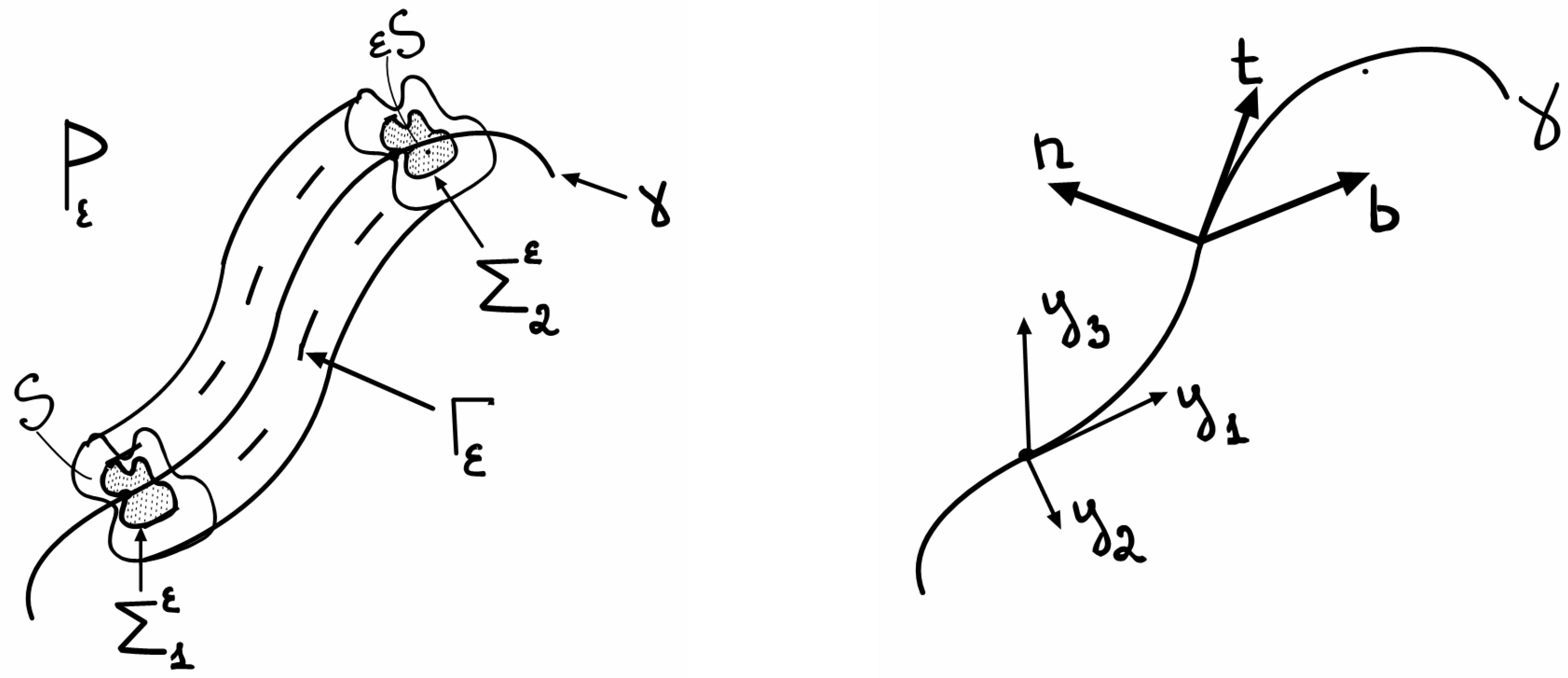
Let us provide a general formulation of the problem according to the work of [14]. Let be a smooth curve (central line of the tube), which is parameterized by arc length , and let be its natural parameterization:
At each point , of the curve , we define the curvature and the Frenet–Serret frame:
where , , and are the tangent vector, normal vector, and binormal vector, respectively. We denote the torsion of the curve with , and we write the Frenet–Serret equations expressing the change of the basis along the curve :
For a smooth domain (cross-section) and a small parameter , we define the undeformed straight tube:
Introducing the notations and , we require the fulfillment of the standard assumption:
which means that the origin “O” is located at the center of gravity of the cross-section S. Assuming that
we define the mapping as
Let us note that , and therefore, assumption (1) implies the injectivity of the mapping . Thus, a bent tube with the central line and the cross-section is defined by the following formula:
The mapping bends the straight tube and transforms it into the bent tube . It should be noted that the curve is located at the center of gravity of each cross-section of the tube, which explains the term “central line”. We denote the beginning and the end of the tube as and , respectively:
We denote the boundary of the tube as and the cross-section of the tube at point as . Figure 1 shows the tube and its center line with the notations introduced above.
3. Equations
The steady flow of viscous incompressible fluid flowing in the tube is described by the Navier–Stokes equations [8,19]:
We assume that the given velocity values at the inlet and outlet of the tube, and , respectively, have the following form:
In order to ensure the well-posedness of the boundary problem, we assume that the functions of prescribed velocities , , and , satisfy the compatibility condition:
Note that the condition on is necessary for the existence of a solution from the space . In physical terms, the relevant and measurable quantity is the flow rate . In the paper [14], it was proved that the global behavior of the flow in a bending tube is determined by the flow rate . Moreover, it was shown in this paper that the influence of the inflow and outflow velocities for is only present in small neighborhoods at the ends of the tube, thus meaning that two flows with different inflow and outflow velocities for and the same flow rate differ only in some small regions near the tube ends.
4. Asymptotic Solution
In this section, we present the asymptotic solution of Equation (2). For the sake of completeness, we briefly describe the proof of this result. For a more complete derivation of the asymptotic solution of Equation (2) and proof of the orders of asymptotic convergence, we refer to [14]. Note that the tube parametrization can be read as , . This allows one to identify the small parameter as the dimensionless diameter of the tube cross-section. First, we define three auxiliary differential problems on the axial cross-section S:
Note that all unknown functions w, , , and q depend on the variables , and the Laplace, divergence, and curl operators are applied accordingly. By solving the boundary problem (3), we define two constants that will appear in the asymptotic solution:
Theorem 1
([14]). The first-order approximation of the solution of the Navier–Stokes Equation (2) in the bent tube has the following form:
This is the Poiseuille flow solution, which describes the flow corresponding to a given flow rate θ. Its convergence order is ε, except for some neighborhood near :
where and C are constants that are independent of ε.
The second-order approximation of the solution of the Navier–Stokes Equation (2) in the bent tube has the following form:
The sum of the first- and second-order approximations has a convergence order of , except for some neighborhood near :
The sum of the first- and second-order approximations for the velocity gradient has a convergence order of :
Now, we schematically describe the proof of this result. The idea is to attach a curvilinear coordinate system to each point and express the Navier–Stokes Equation (2) using these coordinates [20]. First, we define and write down all the auxiliary mathematical objects [21] that will be used to express the Navier–Stokes Equation (2) in the curvilinear coordinate system for the case of a bent tube . The covariant basis, defined by the mapping , contains the vector , and in our case, it takes the following form:
The covariant metric tensor is given by the following:
and the metric . The contravariant basis is defined by the condition , and in the case of a bent tube, it takes the following form:
Thus, the contravariant metric tensor is given by the following:
To determine the covariant derivative ∇, we also need to compute the Christoffel symbols . In this case, the Christoffel symbols are symmetric in the lower indices, where . Due to the definition of the contravariant and covariant basis, there are several zero Christoffel symbols:
and the nonzero symbols have the following expressions in terms of the curvature and torsion :
The remaining nonzero Christoffel symbols can be expressed in terms of the curvature and torsion as follows:
The given text provides important information about the asymptotic behavior of the contravariant metric tensor and the Christoffel symbols . Considering that and , we have the following expressions for the contravariant metric tensor:
where represents the identity matrix, and and are coefficients related to the curvature and torsion of the tube.
The Christoffel symbols are given by the following expressions:
This information allows us to derive the approximation representations (6) and (7). Let be a solution of the Navier–Stokes Equation (2). We introduce the notations:
and we express the velocity vector components in the contravariant basis:
Then, the Navier–Stokes Equation (2) in curvilinear coordinates (see [20]) for the curved tube can be written as follows:
where a summation convention is applied to the repeated lower and upper indices. The covariant derivative in this case acts on the vector field according to the following formula:
We seek the asymptotic expansion for in the following form:
where , , and for the vector function . By sequentially solving these differential problems, we obtain the velocity components , in the contravariant basis and the pressure from expansion (12):
where . Now we obtain the asymptotic solution of the Navier–Stokes Equation (2) in the Frenet–Serret basis by multiplying the velocities by the covariant basis :
5. Calculation of Vorticity
The drag force in the problem of viscous fluid flow can be computed using the following formula [6]:
where , is the kinematic viscosity of the fluid, and p is the pressure. The fluid occupies a volume , is the boundary, and n is the normal to the boundary. is the fluid velocity at the inlet of the channel. In fluid dynamics books [6] and in rigorous mathematical formulations [15], it has been proven that for an incompressible fluid, the formula (13) follows the expression for drag as a volume integral:
In more complex channel geometries, such as a curved channel with an aneurysmal expansion or constriction, vortical zones are formed in the flow. The maintenance of these vortical structures requires additional energy (14).
For the given asymptotic model, let us derive an asymptotic approximation for the vorticity .
Theorem 2.
The first-order approximation of the vorticity for the solution of the Navier–Stokes Equation (2) in the curved tube has the following form:
The second-order approximation of the vorticity for the solution of the Navier-Stokes Equation (2) in the curved tube has the following form:
The sum of the first- and second-order approximations for the vorticity has a convergence order of , except for a small neighborhood near the ends of the tube :
Proof of Theorem 2.
Similarly to the notation in Theorem 1, we introduce the notation for the vorticity of :
and we write the components of the vorticity vector in the contravariant basis as follows:
We seek the asymptotic expansion of the vorticity in the following form:
This form is natural considering the form of the asymptotic expansion of velocity (12) and the rules of differentiation , . We use the well-known formula for computing the vorticity in curvilinear coordinates [20]:
where is the Levi–Civita tensor, including the factor , and are the contravariant coordinates of the velocity vector. Taking into account the asymptotic expansion (10) of the contravariant metric tensor and expanding the formula (15), we have the following:
By substituting the contravariant coordinates of the velocity’s asymptotic expansion [15], we have the following:
and using the Christoffel symbols (9), we obtain the asymptotic expansion of the vorticity in the contravariant basis:
By multiplying the contravariant coordinates of the vorticity vector (16) by the covariant basis and rearranging the terms, we obtain the asymptotic expansion of the vorticity in the basis for the curved tube :
An estimate of the order of convergence follows from an estimate of the order of convergence for the asymptotic expansion of the velocity gradient (8):
The transformations in the inequalities follow from the fact that the rotor operation contains only a part of the derivatives of the gradient operation. □
For a viscous incompressible fluid flow, an important characteristic is the complete dissipation of mechanical energy [19], which depends on the intensity of the vortex inside the region P. From (14), we obtain
where W is the dissipation energy, is the dynamic viscosity, and is the vortex vector. In this model, the dissipation energy W has the order of convergence , which follows from the previous theorem:
Thus, we have obtained an asymptotic approximation of the dissipation energy W for the tube .
6. Circular Cross-Section
For a circular tube, the auxiliary Poisson and Stokes problems (3)–(5) can be solved explicitly, and then we can obtain explicit formulas for the asymptotic approximation of the velocity vector, pressure and vortex vector. Consider a tube that in each axial section will have a circle of radius R, i.e.,
The solution for the auxiliary differential boundary value problem (3)
can be found explicitly, and in the polar coordinates and , it is written as
Then, the auxiliary constants and are respectively equal to
For the second auxiliary differential boundary value problem (4)
we have the solution
Differential problem (5), taking into account the found function w, takes the form
Moving back to the polar coordinates, we obtain a unique solution in the form
By substituting the solutions of auxiliary problems (3)–(5) into formula (6) and then the first-order approximations for velocity and pressure in a tube with a circular section of radius R, we obtain
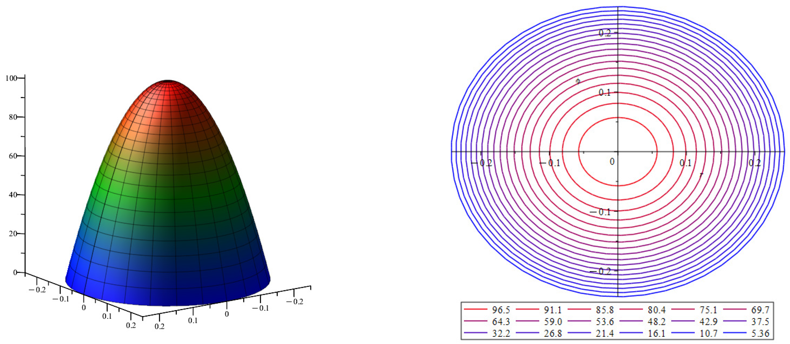
As noted above, this is the Poiseuille flow in a round straight tube [8,19]; the pressure gradient in this case is . The first term of the velocity approximation has a parabolic velocity profile. In Figure 2 on the left is the velocity profile of the first term of the velocity approximation ; on the right are the surface level lines of the velocity profile . Figure 2 describes the approximation of the velocity profile in a thin round straight tube.
Similarly, we substitute the solutions of the problems (3)–(5) into formula (7) and obtain a second-order approximation for the velocity and pressure in a tube with a circular section of radius R:
Thus, for a circular tube, the second term of the approximation of the velocity vector contains only the component with the tangent vector , since the coefficients before the normal and the binormal are zero. As a consequence, the velocity vector in the first and second approximation does not depend on the torsion of the center line .
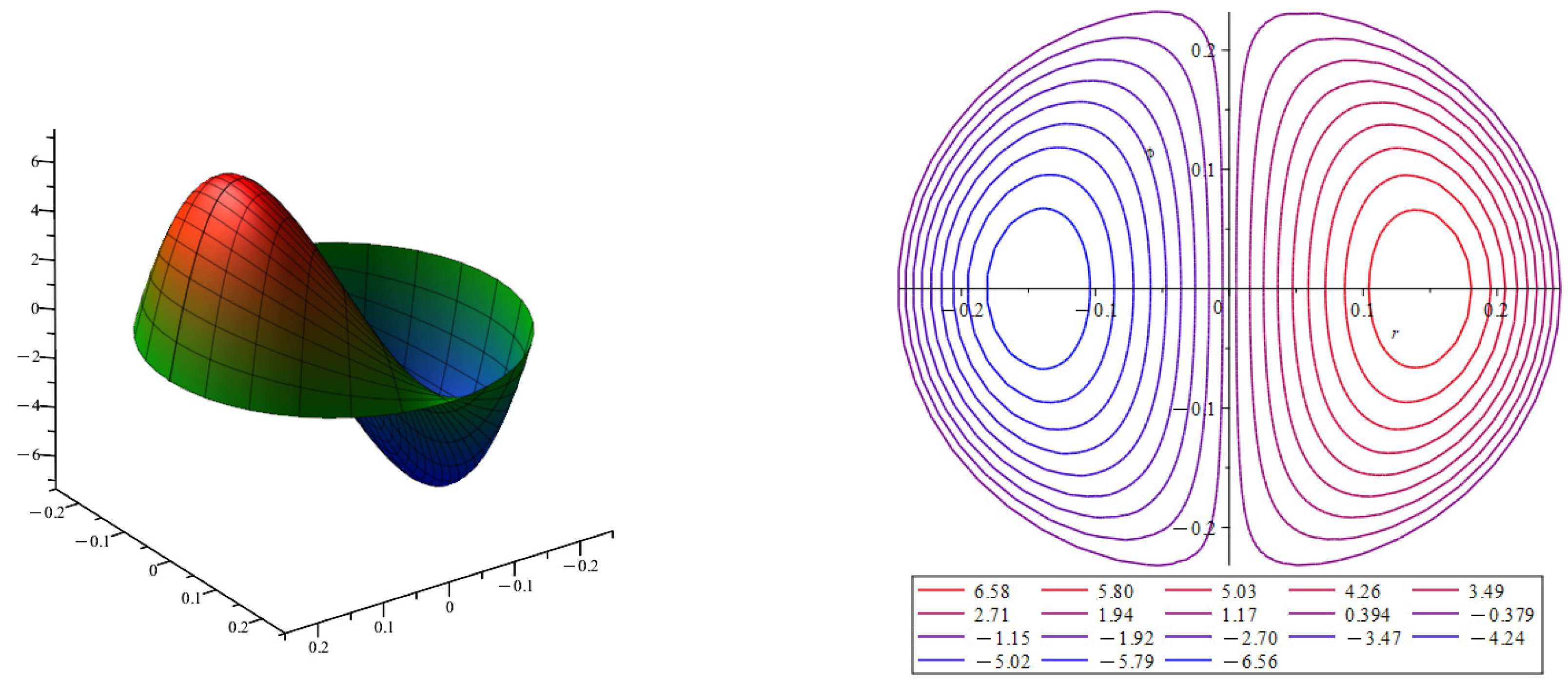
In the presence of the curvature of the central line of the tube , the second term of the velocity approximation is not zero: . In Figure 3 on the left is the velocity profile of the second term of the velocity approximation ; on the right are the surface level lines of the velocity profile . The presence of curvature in a circular tube deflects the velocity flow toward the outer wall of the tube. The flow rate increases on one side and decreases on the other. These are the well-known Dean vortices [6] in hydrodynamics.
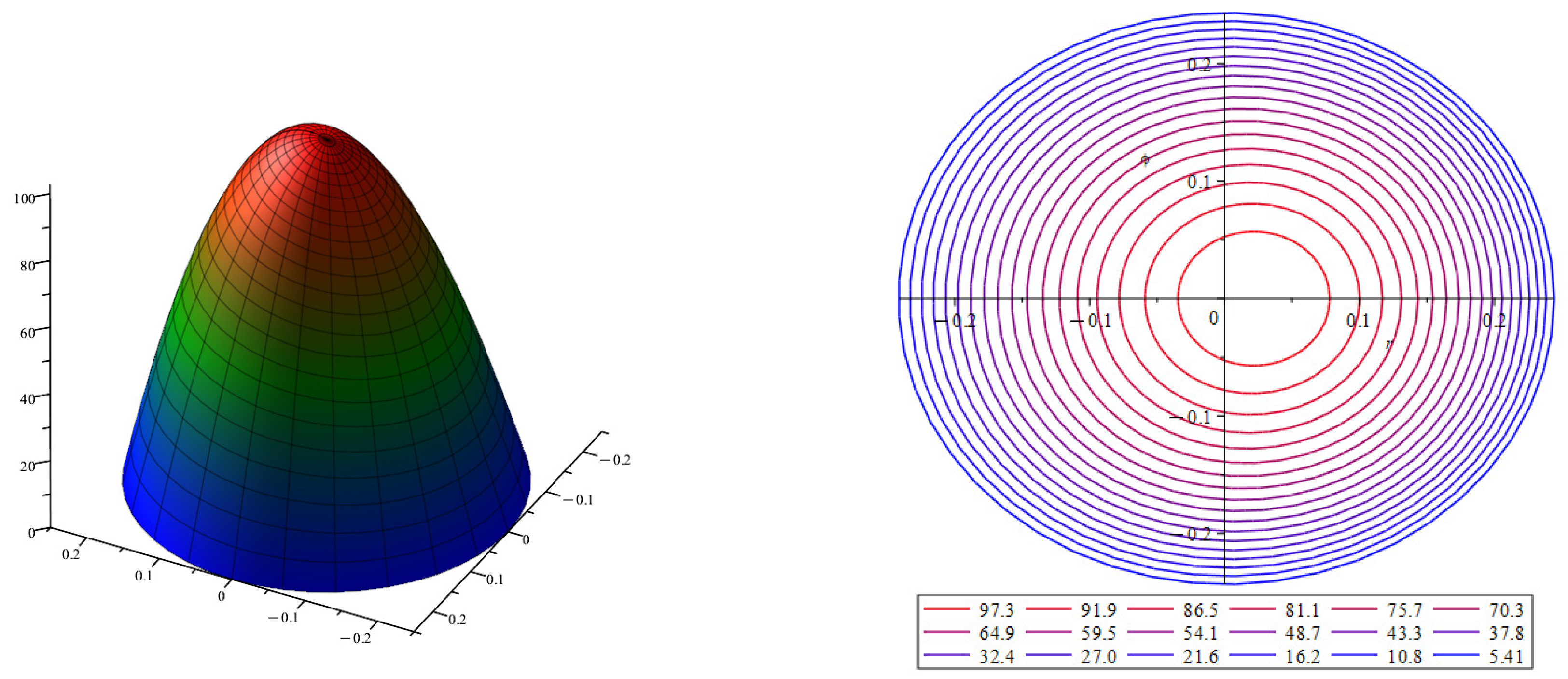
The approximation of the velocity with the order of convergence is calculated as the sum of the first and second approximations . In Figure 4, a velocity profile is presented to approximate the velocity in the section of a curved tube. The surface is shown on the left, and the surface level lines are shown on the right. The velocity profile is calculated for the cross-section of a circular tube with curvature and torsion .
Similarly, for the vortex vector, we substitute the solutions of the problems (3)–(5) into the formulas for the first and second approximations of the vortex vector. The first-order approximation for a vortex in a tube with a circular cross-section of radius R is represented as
and the second-order approximation for a vortex in a tube with a circular section of radius R has the form
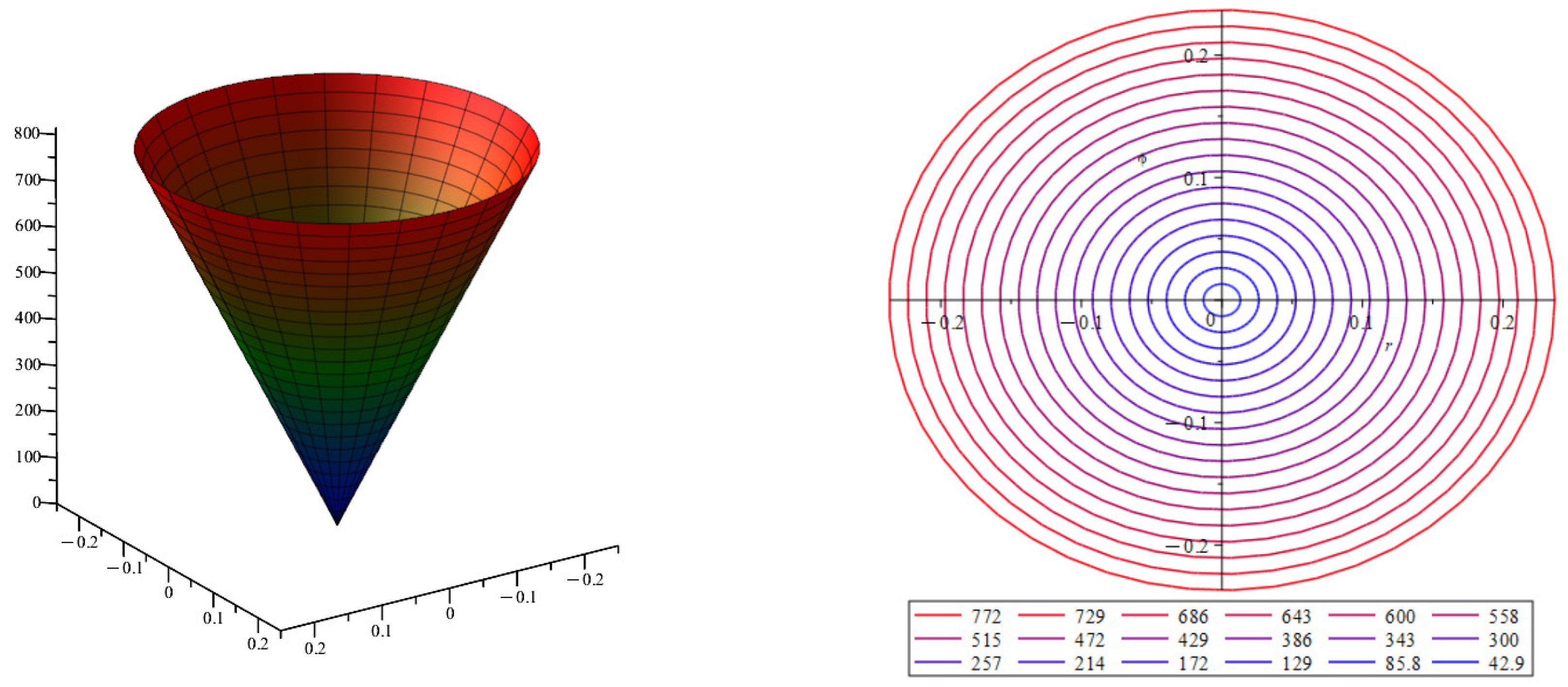
Figure 5 represents the surface of the vortex vector approximation module in the section of a straight thin tube, i.e., the curvature of and the torsion . The vortex takes the smallest value in the center of the tube; its greatest value is reached at the walls of the tube. These facts are consistent with real observations of fluid movement in straight tubes.
The approximation of the vortex with the order of convergence is calculated as the sum of the first and second approximations of the vortex vector . As we can see, the vortex vector, unlike the velocity vector, contains all three components , , and and depends on both the torsion and the curvature of the center line .
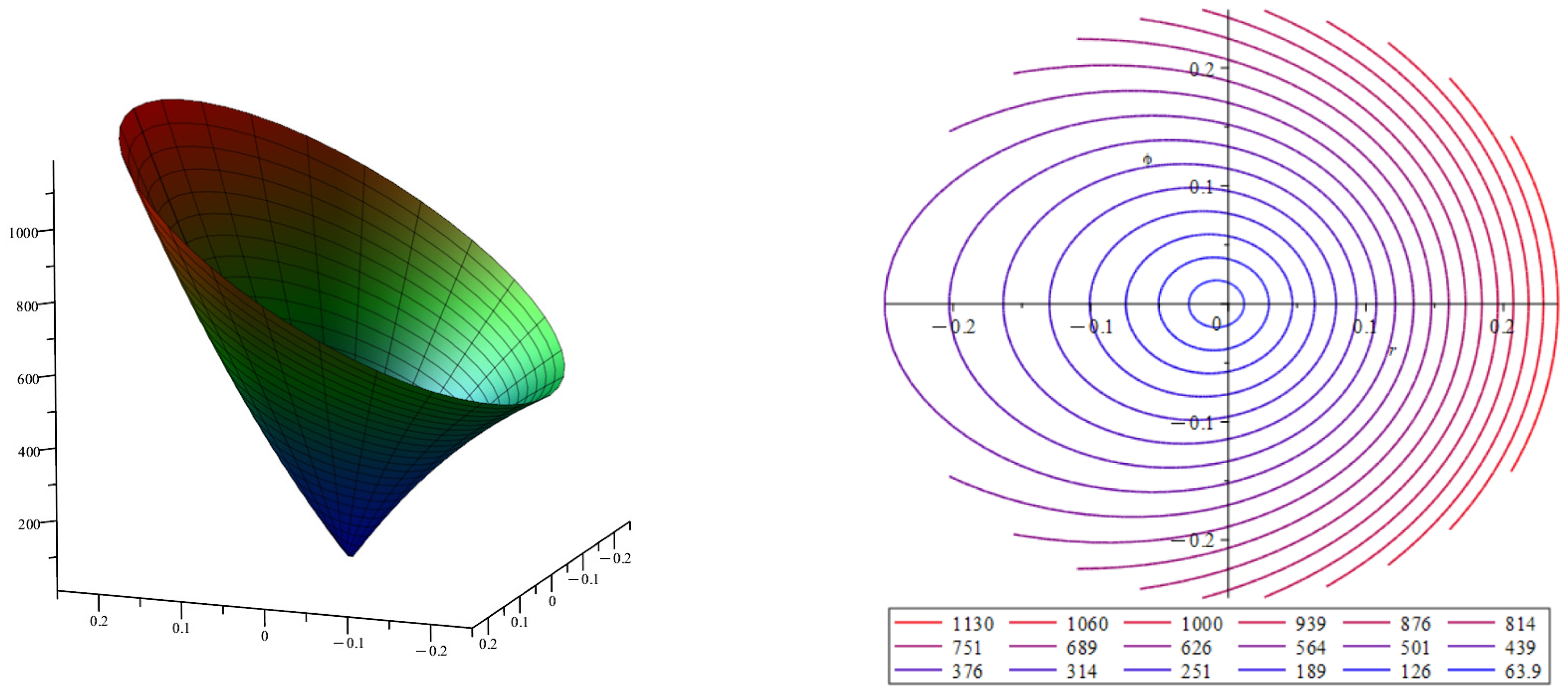
Figure 6 represents the surface of the vortex vector approximation module in a section of a curved tube. The surface is shown on the left; the surface level lines are shown on the right. The approximation modulus of the vortex vector is calculated for the section of a circular tube with curvature and torsion .
As noted earlier, the presence of curvature and torsion significantly deflects the fluid flow. Both the velocity profile and the vortex vector module are rebuilt.
Consider that a round tube of length ℓ with a curvature and a torsion has a constant radius of the section, i.e., the radius of R does not depend on . Calculate the integral of from the square of the modulus of the vortex vector :
The first term of the dissipation energy W corresponds to a round straight tube; the second and third terms of the dissipation energy W correspond to the additional energy arising due to the presence of the curvature and torsion of the center line of the curved tube.
Now, for a circular tube, we can explicitly calculate the velocity vector, pressure, and vortex vector. Note that these values are different for different sections only if the curvature values differ from the torsion at the points of the curve of these sections. Illustrative examples of the velocity profile and the modulus of the vortex vector were presented for a helical circular tube with a cross-section radius R. The fluid flow rate in the initial and final section of the tube is set and constant.
7. Numerical Calculation
For a straight tube with a constant cross-section R, the normalized dissipation energy has the form
where V is the volume of a straight tube. For helicoidal pipes with a constant cross-section R of the normalized dissipation energy up to terms with , they have the form
where V is the volume of a helical tube with a curvature and torsion . Table 1 presents the characteristics of pipes for which the normalized dissipation energy will be calculated next. Note that we identify the small parameter as the dimensionless diameter of the tube cross-section.
Let us calculate the normalized dissipation energy for pipes from the Table 1 using the formulas of (17) and (18). Calculations were carried out for various values of the velocity v in the initial section of the tube, the flow rate in the initial section , and the viscosity of blood Pa·s, with a fluid density of kg/m. Table 2 contains the values of the normalized dissipation energy calculated using the asymptotic formulas of (17) and (18).
To confirm the accuracy of the asymptotic formulas, we performed a numerical calculation of the normalized dissipation energy using the ANSYS program. Table 3 contains the values of the normalized dissipation energy calculated using the ANSYS program.
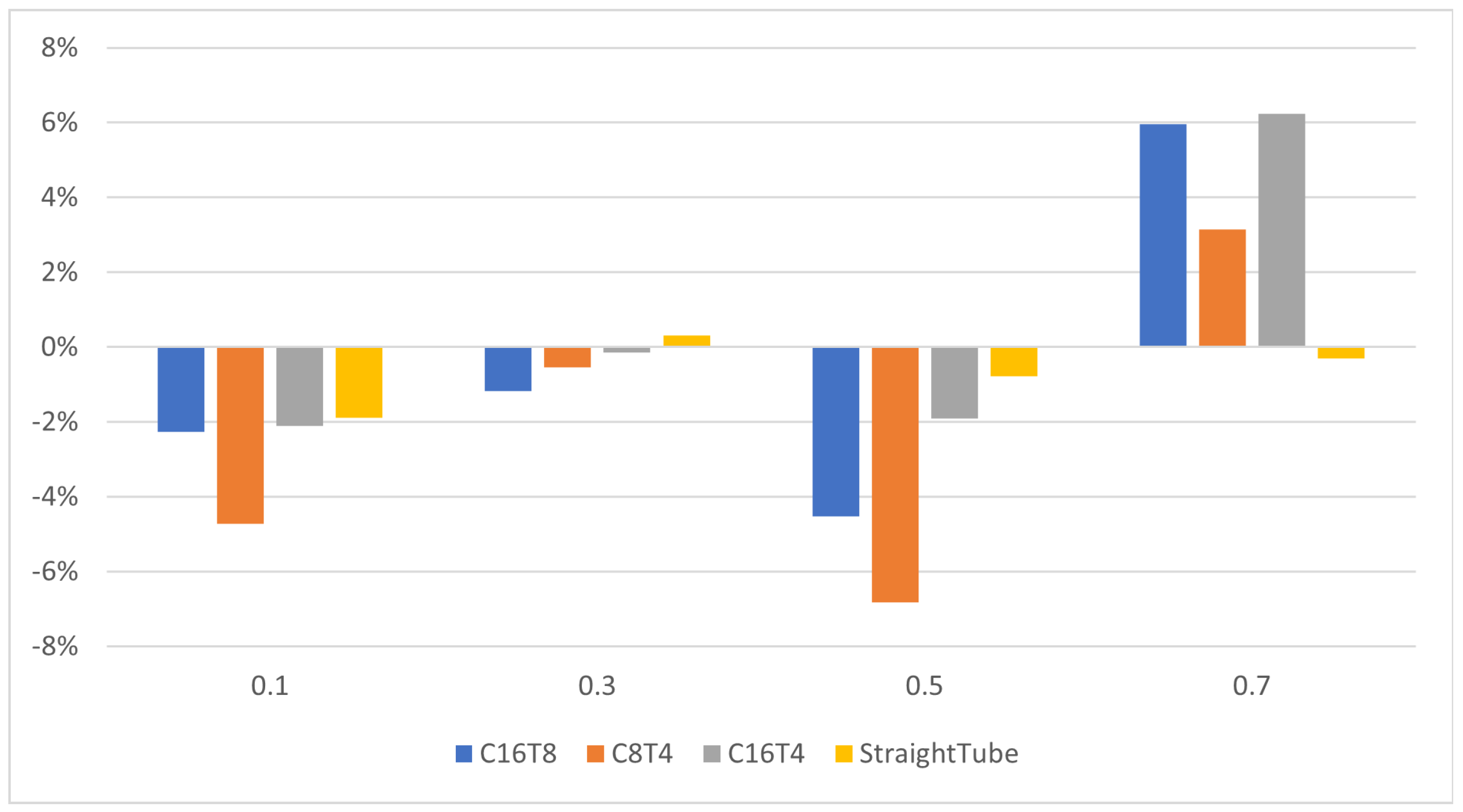
Figure 7 presents the difference in percentages of the normalized dissipation energy calculated using the asymptotic formulas of (17) and (18) and using the ANSYS program.
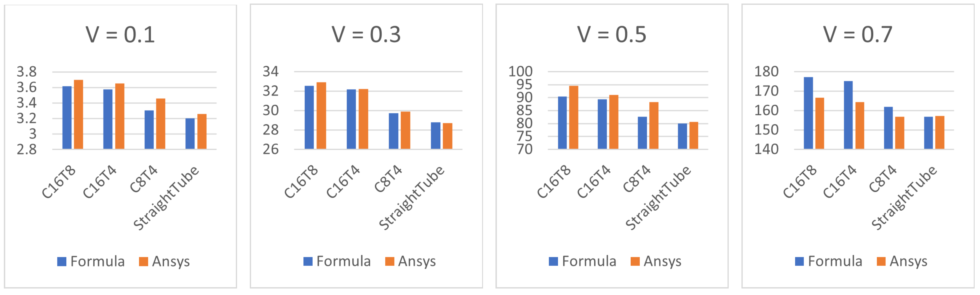
Figure 8 presents the values of the normalized dissipation energy calculated using the asymptotic formulas of (17) and (18) and the ANSYS program.
The above calculations show that the asymptotic formulas for calculating the normalized dissipation energy are quite accurate. The difference in the values of calculated using asymptotic formulas and in the ANSYS package is no more than 6%. For initial velocities in the range from 0.1 to 0.5 m/s, the asymptotic formulas gave lower values of the dissipation energy compared to the values calculated using the ANSYS program. And for initial speeds of more than 0.5 m/s, the opposite trend was observed. This is due to the fact that with an increase in the characteristic flow velocity, the Reynolds number increases, and the transition from a laminar flow type to a turbulent one is carried out. For blood-type fluid, the viscosity of the liquid came out to Pa·s, and the fluid density came out to kg/m. The Reynolds number for the considered tubes with blood-type fluid has the form . Similarly, the Dean number is . So, for the calculated values of and at m/s, we can probably already talk about the turbulent flow regime of the fluid.
8. Conclusions
This study employed asymptotic theory to investigate the behavior of fluid flow in a curved tube. The main contributions of this research include providing representations for the vorticity vector and the energy dissipation in terms of small parameter powers. These formulas enable us to determine the magnitude of vorticity and energy dissipation, which are influenced by the curvature and torsion of the central axis of the channel.
Moreover, the accuracy of the asymptotic formulas was assessed by estimating their performance in terms of small parameter powers. Notably, numerical calculations were conducted for a flow problem in a helical tube, thereby considering various curvature and torsion values. The results of these calculations demonstrate the effectiveness of the asymptotic formulas.
This study underscores the significance of both curvature and torsion in the central axis of the channel in relation to vortex formation and energy dissipation. By considering these geometric parameters, insights into the flow behavior and characteristics can be gained. The obtained theoretical representations and their validation through numerical calculations contribute to a better understanding of the fluid motion in curved channels.
Author Contributions
Conceptualization, A.C. and A.M.; methodology, A.C. and A.M.; software, S.V.; validation, A.C., A.M. and S.V.; formal analysis, A.C., A.M. and S.V.; investigation, A.C., A.M. and S.V.; resources, A.C. and A.M.; data curation, S.V.; writing—original draft preparation, A.M. and S.V.; writing—review and editing, A.C., A.M. and S.V.; visualization, S.V.; supervision, A.C. and A.M.; project administration, A.M.; funding acquisition, A.C. All authors have read and agreed to the published version of the manuscript.
Funding
This research was funded by the Ministry of Education of the Russian Federation through project 14.W03.31.0002 (mathematical formulation and conclusion) and by the Russian Science Foundation through project No 20-71-10034, https://rscf.ru/project/20-71-10034/, accessed on 1 December 2023 (numerical simulations and statistical analysis).
Data Availability Statement
Data are contained within the article. No external sources have been used.
Conflicts of Interest
The authors declare no conflicts of interest.
References
- Tryggeson, H. Analytical Vortex Solutions to the Navier-Stokes Equation. J. Math. Phys. 2008, 49, 113102. [Google Scholar]
- Alastruey, J.; Siggers, J.H.; Peiffer, V.; Doorly, D.J.; Sherwin, S.J. Reducing the data: Analysis of the role of vascular geometry on blood flow patterns in curved vessels. Phys. Fluids 2012, 24, 31902. [Google Scholar] [CrossRef]
- Weiss, D.; Cavinato, C.; Gray, A.; Ramach, A.B.; Avril, S.; Humphrey, J.D.; Latorre, M. Mechanics-driven mechanobiological mechanisms of arterial tortuosity. Sci. Adv. 2020, 6, eabd3574. [Google Scholar] [CrossRef] [PubMed]
- Vassilevski, Y.; Olshanskii, M.; Simakov, S.; Kolobov, A.; Danilov, A. Personalized Computational Hemodynamics: Models, Methods, and Applications for Vascular Surgery and Antitumor Therapy; Elsevier Science: Amsterdam, The Netherlands, 2020. [Google Scholar]
- Kumar, A. Pressure-driven flows in helical pipes: Bounds on flow rate and friction factor. J. Fluid Mech. 2020, 904, A5. [Google Scholar] [CrossRef]
- Schlichting, H.; Gersten, K. Boundary-Layer Theory; Springer: Berlin/Heidelberg, Germany, 2003. [Google Scholar]
- Kobayashi, M.H. On the Navier–Stokes equations on manifolds with curvature. J. Eng. Math. 2008, 60, 55–68. [Google Scholar] [CrossRef]
- Milne-Thomson, L.N. Theoretical Hydrodynamics; The Macmillan and Company: London, UK, 1962. [Google Scholar]
- Shikhmurzaev, Y.; Sisoev, G. Spiralling liquid jets: Verifiable mathematical framework, trajectories and peristaltic waves. J. Fluid Mech. 2017, 819, 352–400. [Google Scholar] [CrossRef]
- Chen, G.Q.; Osborne, D.; Qian, Z. The Navier—Stokes equations with the kinematic and vorticity boundary conditions on non-flat boundaries. Acta Math. Sci. 2009, 29, 919–948. [Google Scholar] [CrossRef]
- Panasenko, G.P.; Stavre, R. Three dimensional asymptotic analysis of an axisymmetric flow in a thin tube with thin stiff elastic wall. J. Math. Fluid Mech. 2020, 22, 35. [Google Scholar] [CrossRef]
- Castineira, G.; Rodriguez, J.M. Asymptotic analysis of a viscous flow in a curved pipe with elastic walls. In Trends in Differential Equations and Applications; Springer: Cham, Switzerland, 2016; pp. 73–87. [Google Scholar]
- Castineira, G.; Marusic-Paloka, E.; Pazanin, I.; Rodriguez, J.M. Rigorous justification of the asymptotic model describing a curved–pipe flow in a time–Dependent domain. Z. Fur Angew. Math. Und Mech. 2019, 99, 1–39. [Google Scholar] [CrossRef]
- Marusic-Paloka, E. The effects of flexion and torsion on a fluid flow through a curved pipe. Appl. Math. Optim. 2001, 44, 245–272. [Google Scholar] [CrossRef]
- Kondoh, T.; Matsumori, T.; Kawamoto, A. Drag Minimization and Lift Maximization in Laminar Flows via Topology Optimization Employing Simple Objective Function Expressions Based on Body Force Integration. Struct. Multidisc. Optim. 2012, 45, 693–701. [Google Scholar] [CrossRef]
- Plotnikov, P.I.; Sokolowski, J. Geometric Aspects of Shape Optimization. J. Geom. Anal. 2023, 33, 206. [Google Scholar] [CrossRef]
- Bello, J.; Fernndez-Cara, E.; Lemoine, J.; Simon, J. The Differentiability of the Drag with Respect to the Variations of a Lipschitz Domain in a Navier-Stokes Flow. SIAM J. Control Optim. 1997, 35, 626–640. [Google Scholar] [CrossRef]
- Garcke, H.; Hinze, M.; Kahle, C.; Lam, K. A phase field approach to shape optimization in Navier-Stokes flow with integral state constraints. Adv. Comput. Math. 2018, 44, 1345–1383. [Google Scholar] [CrossRef]
- Kochin, N.E.; Kibel, I.A.; Roze, N.V. Theoretical Hydromechanics; Interscience Publishers: New York, NY, USA, 1964. [Google Scholar]
- Michal, A.D. Matrix and Tensor Calculus; John Wiley and Sons: New York, NY, USA, 1947. [Google Scholar]
- Kobayashi, S.; Nomizu, K. Foundations of Differential Geometry; Interscience Publishers: New York, NY, USA, 1963. [Google Scholar]
Figure 1.
The tube and its central line .

Figure 2.
The velocity profile for the first term of the velocity approximation is . The color indicates the magnitude of the velocity value, with blue indicating low velocity values and red indicating high velocity values.
Figure 2.
The velocity profile for the first term of the velocity approximation is . The color indicates the magnitude of the velocity value, with blue indicating low velocity values and red indicating high velocity values.

Figure 3.
Velocity profile for the second term of the velocity approximation at . The color indicates the magnitude of the velocity value, with blue indicating low velocity values and red indicating high velocity values.
Figure 3.
Velocity profile for the second term of the velocity approximation at . The color indicates the magnitude of the velocity value, with blue indicating low velocity values and red indicating high velocity values.

Figure 4.
Velocity profile for velocity approximation for curved tube, where and . The color indicates the magnitude of the velocity value, with blue indicating low velocity values and red indicating high velocity values.
Figure 4.
Velocity profile for velocity approximation for curved tube, where and . The color indicates the magnitude of the velocity value, with blue indicating low velocity values and red indicating high velocity values.

Figure 5.
Vortex vector approximation modulus for a straight thin tube. Color indicates the values of vortex vector modulus, with blue indicating low values of vortex vector modulus and red indicating high values.
Figure 5.
Vortex vector approximation modulus for a straight thin tube. Color indicates the values of vortex vector modulus, with blue indicating low values of vortex vector modulus and red indicating high values.

Figure 6.
Velocity profile for velocity approximation and the vortex vector approximation module for curved tube, where and . Color indicates the values of vortex vector modulus, with blue indicating low values of vortex vector modulus and red indicating high values.
Figure 6.
Velocity profile for velocity approximation and the vortex vector approximation module for curved tube, where and . Color indicates the values of vortex vector modulus, with blue indicating low values of vortex vector modulus and red indicating high values.

Figure 7.
The percentage of calculated using asymptotic formulas and calculated using the ANSYS package.
Figure 7.
The percentage of calculated using asymptotic formulas and calculated using the ANSYS package.

Figure 8.
Values of calculated using asymptotic formulas and calculated using the ANSYS package.


Table 1.
Designations and characteristics of pipes.
| Notation | Curvature , 1/m | Torsion , 1/m | Length ℓ, m | Radius of Section R, m |
|---|---|---|---|---|
| C16T8 | 16 | 8 | 2.24 | 0.02 |
| C16T4 | 16 | 4 | 4.12 | 0.02 |
| C8T4 | 8 | 4 | 2.24 | 0.02 |
| Straight Tube | 0 | 0 | 1 | 0.02 |
Table 2.
The values of calculated using asymptotic formulas.
| Input Velocity v, m/s | C16T8 | C16T4 | C8T4 | Straight Tube |
|---|---|---|---|---|
| 0.1 | 3.6 | 3.6 | 3.3 | 3.2 |
| 0.3 | 32.5 | 32.2 | 29.7 | 28.8 |
| 0.5 | 90.4 | 89.4 | 82.6 | 80.0 |
| 0.7 | 177.2 | 175.2 | 161.9 | 156.8 |
Table 3.
The values of calculated using the ANSYS program.
| Input Velocity v, m/s | C16T8 | C16T4 | C8T4 | Straight Tube |
|---|---|---|---|---|
| 0.1 | 3.7 | 3.7 | 3.5 | 3.3 |
| 0.3 | 32.9 | 32.2 | 29.9 | 28.7 |
| 0.5 | 94.5 | 91.1 | 88.2 | 80.6 |
| 0.7 | 166.7 | 164.3 | 156.8 | 157.3 |
Disclaimer/Publisher’s Note: The statements, opinions and data contained in all publications are solely those of the individual author(s) and contributor(s) and not of MDPI and/or the editor(s). MDPI and/or the editor(s) disclaim responsibility for any injury to people or property resulting from any ideas, methods, instructions or products referred to in the content. |
© 2024 by the authors. Licensee MDPI, Basel, Switzerland. This article is an open access article distributed under the terms and conditions of the Creative Commons Attribution (CC BY) license (https://creativecommons.org/licenses/by/4.0/).
Share and Cite
MDPI and ACS Style
Chupakhin, A.; Mamontov, A.; Vasyutkin, S. Asymptotic Representation of Vorticity and Dissipation Energy in the Flux Problem for the Navier–Stokes Equations in Curved Pipes. Axioms 2024, 13, 65. https://doi.org/10.3390/axioms13010065
AMA Style
Chupakhin A, Mamontov A, Vasyutkin S. Asymptotic Representation of Vorticity and Dissipation Energy in the Flux Problem for the Navier–Stokes Equations in Curved Pipes. Axioms. 2024; 13(1):65. https://doi.org/10.3390/axioms13010065
Chicago/Turabian StyleChupakhin, Alexander, Alexander Mamontov, and Sergey Vasyutkin. 2024. "Asymptotic Representation of Vorticity and Dissipation Energy in the Flux Problem for the Navier–Stokes Equations in Curved Pipes" Axioms 13, no. 1: 65. https://doi.org/10.3390/axioms13010065
Note that from the first issue of 2016, this journal uses article numbers instead of page numbers. See further details here.