Numerical Reconstruction of the Source in Dynamical Boundary Condition of Laplace’s Equation

Abstract

In this work, we consider Cauchy-type problems for Laplace’s equation with a dynamical boundary condition on a part of the domain boundary. We construct a discrete-in-time, meshless method for solving two inverse problems for recovering the space–time-dependent source and boundary functions in dynamical and Dirichlet boundary conditions. The approach is based on Green’s second identity and the forward-in-time discretization of the non-stationary problem. We derive a global connection that relates the source of the dynamical boundary condition and Dirichlet and Neumann boundary conditions in an integral equation. First, we perform time semi-discretization for the dynamical boundary condition into the integral equation. Then, on each time layer, we use Trefftz-type test functions to find the unknown source and Dirichlet boundary functions. The accuracy of the developed method for determining dynamical and Dirichlet boundary conditions for given over-determined data is first-order in time. We illustrate its efficiency for a high level of noise, namely, when the deviation of the input data is above 10% on some part of the over-specified boundary data. The proposed method achieves optimal accuracy for the identified boundary functions for a moderate number of iterations.

1. Introduction

Elliptic partial differential equations (PDEs) with dynamical boundary conditions, imposed on the whole or part of the domain boundary, describe processes of filtration in various fields, including hydrology, chemistry, semi-conductors, and heat transfer in a solid in contact with a fluid (see, e.g., refs. [1,2,3]).

Global existence results for 2D elliptic equations with dynamical boundary conditions are obtained in ref. [2,4]. The existence of blow-up solutions to Laplace’s equation with semi-linear dynamical boundary conditions is studied in refs. [5]. The authors of [6,7] derived estimates of the convergence rate compatible with the smoothness of the differential solutions to the Poisson’s equation with a dynamical interface and dynamic boundary condition in special discrete Sobolev norms. In ref. [8], a weighted finite difference scheme is constructed and studied for a numerical solution of Laplace’s equation with dynamical boundary conditions.

Numerical identification source problems in mathematical physics using experimental data have garnered great interest in recent decades (see, e.g., refs. [9,10,11,12,13,14]). Such inverse problems belong to the class of ill-posed problems and their numerical analysis requires special numerical identification techniques, such as the quasi-solution method, selection method, iterative optimization algorithms, and regularization procedures [11,12,13,14,15,16,17,18,19]. Among them, the most popular is Tikhonov’s regularization method [20,21].

The inverse Cauchy problem for PDEs is to recover the missing boundary data from given over-specified Dirichlet or Neumann data on a part of the domain boundary. Being ill-posed [22], it usually requires regularization techniques for numerically handling the instability.

Inverse Cauchy problems for Laplace’s and Poisson’s equations can be used for imaging corrosion damage in plates from electrostatic data (see, e.g., the references in ref. [17]), for crack processes in elasticity [13,23], and thermal processes [24,25]. An interesting engineering model that considers energy systems as full cells is described by an unknown boundary data inverse problem for a Poisson’s equation in ref. [26]. Feyman’s PDEs problem [27] is an inverse Cauchy problem with dynamical boundary conditions, describing gravity capillary waves.

In this paper, we consider two inverse boundary source problems for Laplace’s equation with a dynamical condition on a part of the boundary. We determine the Dirichlet boundary condition and source in the dynamical boundary condition under Dirichlet–Neumann over-determined data.

Analytical results for inverse boundary condition identification (inverse Cauchy-type) problems for elliptic PDEs, or particularly for Laplace’s equation, were proposed, for example, in refs. [19,28,29,30]. A unique reconstruction of a constant heat transfer coefficient was achieved in ref. [30] from a singular boundary energy measurement within a non-linear Robin-type boundary condition linked to an elliptic equation. The existence and uniqueness of the inverse source problem for elliptic equations were proved in ref. [19]. Moreover, the continuous dependence of the inverse problem solution from the observations was established. In ref. [28], the author reviews some open direct and inverse parabolic–elliptic Laplace-type problems. In addition, the uniqueness of the Cauchy inverse coefficient problem for elliptic equations, with a focus on Poisson’s equation, is discussed in [29].

Various numerical methods have been developed for solving the inverse Cauchy problem for elliptic PDEs. For example, the Mann iterative regularization method in [31], the Kozlov–Maz’ya–Fomin algorithm [32] was employed in ref. [26] to identify missing boundary data for a 2D diffusion-reaction PDE, the coupled complex boundary method was used in [33] to solve inverse Cauchy problems for a kind of elliptic PDE, and the collocation method, where the collocation points are determined based on the Chebyshev nodes, was used in [24] for solving Cauchy-type problems for Laplace’s equation. The authors of [34] discuss the reconstruction of the Robin boundary condition by recovering the Robin coefficient from given Cauchy data. This problem describes a process of electric impedance tomography in which the electrical potential is the solution of Laplace’s equation.

Meshless methods are widely used for solving inverse Cauchy and source problems for elliptic equations. The local meshless technique, based on the finite collocation method for solving Cauchy problems of elliptic PDEs in annulus domains, was developed in ref. [35]. A novel meshless numerical solution method for the inverse Cauchy problem for a semi-linear elliptic-type PDE in an arbitrary doubly connected plane domain was developed in [36]. Meshless and iteration free methods, based on a collocation scheme using radial basis functions, for solving the inverse wave problem for boundary identification and for recovering the source term were proposed in refs. [37,38]. The radial basis collocation method was used in ref. [39] for solving the parameter identification inverse Helmholtz problem. In ref. [40], the authors constructed a numerical method for solving the inverse Cauchy problem in a two-layered domain.

The method of fundamental solutions (MFS) is a meshless boundary collocation method that belongs to the family of Trefftz methods [41]. In recent years, there has been a lot of activity regarding the application of MFS for solving inverse problems. A brief review of inverse Cauchy problems for Laplace’s and Poisson’s equations is presented in refs. [13,41].

One notorious approach for solving inverse Cauchy problems of PDEs is the use of Green’s identity to obtain global functional dependence for deriving the unknown boundary data from other boundary data.

The authors of [23] used Green’s formula to transform the inverse problem into a moment problem for the numerical computation of a Cauchy problem. The second Green’s identity was employed in refs. [18,42] to solve one-dimensional source and boundary condition inverse problems.

In ref. [42], the inverse heat conduction problem for identifying two boundary functions for given additional observations of the temperature was solved. Using the adjoint Trefftz method, the authors constructed a global boundary integral equation method (BIEM). A global domain BIEM was constructed in ref. [18] to restore the space–time-dependent heat source under the measurements of the boundary and final time condition.

Based on the second Green’s identity, the author of [17] developed a global domain boundary integral equation method for Laplace’s and Poisson’s equations. Then, they used the integral equation and Trefftz functions to solve the inverse Cauchy problem for recovering unknown boundary conditions and the inverse source problem for Poisson’s equation.

Fewer results in the literature are related to the numerical solution of inverse problems, especially inverse Cauchy problems for PDEs with dynamical boundary conditions. In ref. [43], the authors studied the inverse problem of numerically determining the initial temperatures in a heat equation with dynamical boundary conditions under additional data after a final time. The inverse problem was reduced to a Tikhonov minimization problem. The authors of ref. [15] investigated the inverse problem for a heat equation with dynamic boundary conditions for determining two source terms under final time observations. They applied the weak solution approach to a construct gradient formula of the cost functional and the corresponding adjoint problem. A numerical algorithm was also proposed. An inverse problem of a weakly coupled parabolic–elliptic system with dynamical boundary was studied in ref. [27]. This is a Cauchy problem for water waves, which was first proposed by Richard Feynman.

In this work, we extend the ideas in ref. [17] and solve two inverse problems for recovering space–time-dependent boundary functions in Laplace’s problem with a dynamical boundary condition.

The remaining part of the paper is organized as follows. In Section 2, the forward (direct) problem is formulated and its well-posedness is discussed. In Section 3, using the second Green’s identity for the forward problem, we obtain the basic relation between the dynamical boundary source, the boundary conditions, and the other input data. The main results of the paper, concerning inverse problems are obtained in Section 4. Section 5 is devoted to the numerical test examples, which illustrate the efficiency of the proposed algorithm. Some strengths, weaknesses, and limitations of the method are discussed in Section 6. The paper finishes with some concluding remarks.

2. The Forward Problem

Let us introduce the rectangular spatial domain $\overline{\mathsf{\Omega }}=\{(x,y):0\le x\le l_1,0\le y\le l_2\}$ with boundary $\mathsf{\Gamma }=\overline{\mathsf{\Omega }}\setminus \mathsf{\Omega }$, where $\mathsf{\Omega }=\{(x,y):0<x<l_1,0<y<l_2\}$. Let us denote the lower/south boundary as ${\mathsf{\Gamma }}_0=\{(x,y):0<x<l_1,y=0\}$. Let T be the final time and $t\in [0,T]$ be the time variable. We consider the initial-boundary value problem for the unknown function $u(x,y,t)$

$$\begin{array}{ccc}& & ▵u=0,(x,y)\in \mathsf{\Omega },t\in (0,T),\hfill \end{array}$$

(1)

$$\begin{array}{ccc}& & \frac{\partial u}{\partial t}=\frac{\partial u}{\partial y}+g(x,t),(x,y)\in {\mathsf{\Gamma }}_0,t\in (0,T),\hfill \end{array}$$

(2)

$$\begin{array}{ccc}& & u(0,y,t)=u_W(y,t),y\in [0,l_2],t\in (0,T),\hfill \end{array}$$

(3)

$$\begin{array}{ccc}& & u(x,l_2,t)=u_N(x,t),x\in [0,l_1],t\in (0,T),\hfill \end{array}$$

(4)

$$\begin{array}{ccc}& & u(l_1,y,t)=u_E(y,t),y\in [0,l_2],t\in (0,T),\hfill \end{array}$$

(5)

$$\begin{array}{ccc}& & u(x,0,0)=u_0\left(x\right),x\in [0,l_1],\hfill \end{array}$$

(6)

where $▵=\frac{{\partial }^2}{\partial x^2}+\frac{{\partial }^2}{\partial y^2}$ is the Laplacian, $g(x,t)$, $u_W(y,t)$, $u_E(y,t)$, $u_N(x,t)$, and $u_0\left(x\right)$ are smooth known functions. Moreover, we assume that the following compatibility conditions are fulfilled:

$$\begin{array}{cc}& {\displaystyle u_E(l_2,t)=u_N(l_1,t),u_W(l_2,t)=u_N(0,t),u_W(0,0)=u_0\left(0\right),u_E(0,0)=u_0\left(l_1\right),}\\ & \\ & {\displaystyle \frac{\partial u_W}{\partial t}(0,t)=\frac{\partial u_W}{\partial y}(0,t)+g(0,t),\frac{\partial u_E}{\partial t}(l_1,t)=\frac{\partial u_E}{\partial y}(l_1,t)+g(l_1,t),t>0.}\end{array}$$

(7)

Such problems arise in hydrology. For example, the filtration problem for the pressure in the steady-state filtration equation and the dynamic upper edge layer are accounted for by a non-stationary boundary condition (see, e.g., refs. [2,3] and the references therein).

Results of weak solutions of problems like (1)–(6) were obtained in refs. [6,7]. Our computational method requires the existence of global smooth solutions. The existence of global classical solutions for elliptic equations with dynamical boundary conditions was proved in refs. [2,44,45,46,47]. Modifying the results in [47], we can easily obtain the following assertion of the global existence and uniqueness of the solution of (1)–(6).

Theorem 1. 

We assume that $g\in C^1\left(Q_T\right)$, $Q_T=\mathsf{\Omega }\times (0,T)$, $\mathsf{\Omega }={\mathsf{\Omega }}_1\times {\mathsf{\Omega }}_2$, ${\mathsf{\Omega }}_i=(0,l_i)$, $i=1,2$ and $u_W$, $u_E\in C^1\left({\mathsf{\Omega }}_{2T}\right)$, $u_N\in C^1\left({\mathsf{\Omega }}_{1T}\right)$, ${\mathsf{\Omega }}_{iT}={\mathsf{\Omega }}_i\times (0,T)$, $i=1,2$, $u_0\in C^2\left({\mathsf{\Omega }}_1\right)$. Also, we suppose that the compatibility conditions (7) hold. Then, for every T, $0<T<\infty$, there exists a unique solution $u\in C\left((0,T),C^2\left(\overline{\mathsf{\Omega }}\right)\right)$ to problems (1)–(6).

Proof. 

We use the results from Section 3 of [47], where $\mathsf{\Gamma }$ is the boundary of the domain $\overline{\mathsf{\Omega }}$. In our case, the compatibility conditions assure the existence and uniqueness of a smooth solution to problems (1)–(7). □

3. Basic Identities

In this section, we apply the second Green’s identity to problems (1)–(6) in order to obtain a global relation between the source $g(x,t)$, the boundary functions, and the other input data.

We start with recalling the well-known Green’s theorem in the plane.

Lemma 1 

(Green’s theorem in the plane [17]). Let Ω be a bounded region in the plane $(x,y)$ with a counter-clockwise contour Γ consisting of finitely many smooth curves. Let $G_1(x,y)$ and $G_2(x,y)$ be functions that are differentiable in Ω and continuous in $\overline{\mathsf{\Omega }}$. Then,

$$\underset{\mathsf{\Omega }}{\int }\int \left[\frac{\partial G_2}{\partial x}-\frac{\partial G_1}{\partial y}\right]dxdy={\oint }_{\mathsf{\Gamma }}(G_{1}dx+G_{2}dy).$$

(8)

Taking

$$G_1=v\frac{\partial u}{\partial y}-u\frac{\partial v}{\partial y},G_2=u\frac{\partial v}{\partial x}-v\frac{\partial u}{\partial x},$$

in (8), we obtain the second Green’s identity for the Laplace operator.

Theorem 2 

(Second Green’s identity [17]). Let Ω be a bounded domain in the plane $(x,y)$ with a counter-clockwise contour Γ consisting of a finite number of smooth curves. Let $u(x,y)$ and $v(x,y)$ be functions that are twice differentiable in Ω and continuous on $\overline{\mathsf{\Omega }}$. Then,

$$\underset{\mathsf{\Omega }}{\int }\int (u▵v-v▵u)={\oint }_{\mathsf{\Gamma }}\left(u\frac{\partial v}{\partial n}-v\frac{\partial u}{\partial n}\right)ds,$$

(9)

where $d\sigma =dxdy$ is an area derivative with respect to $\overrightarrow{n}=\left(\frac{dy}{ds},-\frac{dx}{ds}\right).$

Theorem 3 

(Global relation). For problems (1)–(6), the following global relation holds:

$$\begin{array}{c}\hfill \begin{array}{cc}\hfill \oint \left(u\frac{\partial v}{\partial n}-v\frac{\partial u}{\partial n}\right)ds=& {\int }_0^{l_1}\left[\left(\frac{\partial u}{\partial t}(x,0,t)-g(x,t)\right)v(x,0)-u(x,0,t)\frac{\partial v}{\partial y}(x,0)\right]dx\hfill \\ & +{\int }_0^{l_2}\left[u(l_1,y,t)\frac{\partial v}{\partial x}(l_1,y)-v(l_1,y)\frac{\partial u}{\partial x}(l_1,y,t)\right]dy\hfill \\ & -{\int }_0^{l_1}\left[\frac{\partial u}{\partial y}(x,l_2,t)v(x,l_2)-u(x,l_2,t)\frac{\partial v}{\partial y}(x,l_2)\right]dx\hfill \\ & -{\int }_0^{l_2}\left[u(0,y,t)\frac{\partial v}{\partial x}(0,y)-v(0,y)\frac{\partial u}{\partial x}(0,y,t)\right]dy=0,\hfill \end{array}\end{array}$$

(10)

for any function v with $▵v=0$.

Proof. 

Inserting $▵v=0$ into (9), integrating along the contour $\mathsf{\Gamma }={\mathsf{\Gamma }}_0\cup {\mathsf{\Gamma }}_1\cup {\mathsf{\Gamma }}_2\cup {\mathsf{\Gamma }}_3$, where ${\mathsf{\Gamma }}_1=\{(x,y):x=l_1,0\le y\le l_2\}$, ${\mathsf{\Gamma }}_2=\{(x,y):y=l_2,0\le x\le l_1\}$, ${\mathsf{\Gamma }}_3=\{(x,y):x=0,0\le y\le l_2\}$ and taking into account the boundary condition (2), we obtain (10). □

Now, after the time-discretization of the dynamical boundary condition on each time level, we can solve inverse problems for the elliptic equation using the approach in ref. [17].

4. Inverse Problems

In this section, we formulate inverse problems for identifying space–time-dependent boundary functions in Laplace’s problems (1)–(6). Then, after the time discretization of the dynamical problems, we use the results in Section 3 and ref. [17] to solve them numerically using the space-meshless approach.

The first inverse problem, denoted by $\mathbf{IP}-{\mathbf{gu}}_{{\mathsf{\Gamma }}_{\mathbf{0}}}$, concerns recovering the function $g(x,t)$ and $u(x,0,t)$ in (1)–(6), under the additional observation

$$\frac{\partial u}{\partial y}(x,l_2,t)={\tilde{u}}_N(x,t),x\in [0,l_1],t\in (0,T),$$

(11)

where ${\tilde{u}}_N(x,t)$ is a measured function. Additionally, the compatibility condition holds as follows:

$$\frac{\partial u_W}{\partial y}(l_2,t)={\tilde{u}}_N(0,t).$$

The second inverse problem, referred to as $\mathbf{IP}-{\mathbf{gu}}_{{\mathsf{\Gamma }}_{\mathbf{0}}}{\mathbf{u}}_{\mathbf{W}}$, is to determine the functions $g(x,t)$, $u(x,0,t)$, and $u_W(y,t)$ in (1)–(6) for given measurements (11).

Such inverse Cauchy problems are challenging to solve even numerically because their solution does not depend continuously on the input data [17].

First, we apply time semi-discretization to (10). Let us introduce a uniform time mesh with grid nodes $t_n=n\tau$, $n=0,1,\dots ,M$, $\tau =T/M$. Thus, applying the forward Euler method to the dynamical boundary condition (2), we obtain

$$\frac{u^{n+1}-u^n}{\tau }=\frac{\partial u^{n+1}}{\partial y}+g(x,t_{n+1}),(x,y)\in {\mathsf{\Gamma }}_0,t\in (0,T),$$

(12)

where $u^n:=u^n(x,y)=u(x,y,t_n)$.

Considering (10) at the time layer $t_{n+1}$ and applying (12), we derive

$$\begin{array}{c}\hfill \begin{array}{cc}\hfill & {\int }_0^{l_1}\left[\left(\frac{u^{n+1}(x,0)-u^n(x,0)}{\tau }-g(x,t_{n+1})\right)v(x,0)-u^{n+1}(x,0)\frac{\partial v}{\partial y}(x,0)\right]dx\hfill \\ & +{\int }_0^{l_2}\left[u^{n+1}(l_1,y)\frac{\partial v}{\partial x}(l_1,y)-v(l_1,y)\frac{\partial u^{n+1}}{\partial x}(l_1,y)\right]dy\hfill \\ & -{\int }_0^{l_1}\left[\frac{\partial u^{n+1}}{\partial y}(x,l_2)v(x,l_2)-u^{n+1}(x,l_2)\frac{\partial v}{\partial y}(x,l_2)\right]dx\hfill \\ & -{\int }_0^{l_2}\left[u^{n+1}(0,y)\frac{\partial v}{\partial x}(0,y)-v(0,y)\frac{\partial u^{n+1}}{\partial x}(0,y)\right]dy=0.\hfill \end{array}\end{array}$$

(13)

4.1. Solution of $\mathit{IP}-{\mathit{gu}}_{{\Gamma }_{\mathit{0}}}$

To construct the numerical algorithm for solving the inverse problem, following [17], we suggest a trial solution using test functions that satisfy Laplace’s equation, despite the initial conditions, boundary conditions, and over-determined data.

From Theorem 3 and [17] at each time layer, we take one and the same test function $v(x,y)$, which is a stable solution of (1):

$${\displaystyle v(x,y)=sin\frac{k\pi x}{l_1}{e}^{-k\pi y/l_1},k\in \mathbb{N}.}$$

(14)

For $k\in \mathbb{N}$, these functions are similar to the well-known Trefftz functions [41]. Following [17], we refer to the proposed approach as the Trefftz test function method.

Further, from (13) and (14), we obtain

$$\begin{array}{c}\hfill \begin{array}{cc}& {\int }_0^{l_1}\left[\frac{u^{n+1}(x,0)-u^n(x,0)}{\tau }-g(x,t_{n+1})+\frac{k\pi }{l_1}{u}^{n+1}(x,0)\right]sin\frac{k\pi x}{l_1}dx\hfill \\ \hfill =& {\int }_0^{l_1}\left[\frac{\partial u^{n+1}}{\partial y}(x,l_2)v(x,l_2)-u^{n+1}(x,l_2)\frac{\partial v}{\partial y}(x,l_2)\right]dx\hfill \\ & +{\int }_0^{l_2}\left[u^{n+1}(0,y)\frac{\partial v}{\partial x}(0,y)-u^{n+1}(l_1,y)\frac{\partial v}{\partial x}(l_1,y)\right]dy.\hfill \end{array}\end{array}$$

Consequently, from (3)–(5) and (11), we derive

$$\begin{array}{c}\hfill \begin{array}{cc}\hfill & {\int }_0^{l_1}\left[\left(\frac{k\pi }{l_1}+\frac{1}{\tau }\right)u^{n+1}(x,0)-g(x,t_{n+1})\right]sin\frac{k\pi x}{l_1}dx\hfill \\ \hfill =& {\int }_0^{l_1}\frac{u^n(x,0)}{\tau }sin\frac{k\pi x}{l_1}dx\hfill \\ & +{\int }_0^{l_1}\left[{\tilde{u}}_N^{n+1}\left(x\right)v(x,l_2)-u_N^{n+1}\left(x\right)\frac{\partial v}{\partial y}(x,l_2)\right]dx\hfill \\ & +{\int }_0^{l_2}\left[u_W^{n+1}\left(y\right)\frac{\partial v}{\partial x}(0,y)-u_E^{n+1}\left(y\right)\frac{\partial v}{\partial x}(l_1,y)\right]dy:=f_k^{n+1}.\hfill \end{array}\end{array}$$

(15)

Therefore, since $f_k^{n+1}$ is known, we can determine $u^{n+1}(x,0)$ and $g^{n+1}\left(x\right)$ from

$${\int }_0^{l_1}\left[\left(\frac{k\pi }{l_1}+\frac{1}{\tau }\right)u^{n+1}(x,0)-g^{n+1}\left(x\right)\right]sin\frac{k\pi x}{l_1}dx=f_k^{n+1}.$$

(16)

Representing the unknown functions by

$$\begin{array}{c}\hfill \begin{array}{cc}\hfill & u^n(x,0)=a_0^n+\sum _{j=1}^m{a}_j^{n}cos\left(jx\right)+\sum _{j=1}^m{b}_j^{n}sin\left(jx\right),\hfill \\ & g^n\left(x\right)=c_0^n+\sum _{j=1}^m{c}_j^{n}cos\left(jx\right)+\sum _{j=1}^m{d}_j^{n}sin\left(jx\right),\hfill \end{array}\end{array}$$

(17)

at each time level, the recovery reduces to the determination of $m_1=4m+2$ coefficients, i.e., the elements of the vector

$${\mathbf{e}}^n={[a_1^n,a_2^n,\dots ,a_m^n,b_1^n,b_2^n,\dots ,b_m^n,a_0^n,c_1^n,c_2^n,\dots ,c_m^n,d_1^n,d_2^n,\dots ,d_m^n,c_0^n]}^T.$$

We take $m_1$ test functions (14) at each time step. Substituting (17) in (16), we obtain the linear system

$$\mathbf{A}{\mathbf{e}}^{n+1}={\mathbf{f}}^{n+1},{\mathbf{f}}^n={[f_1^n,f_2^n,\dots ,f_{m_1}^n]}^T,$$

(18)

where $\mathbf{A}$ is the $m_1\times m_1$ coefficient matrix with elements

$$\begin{array}{ccc}& & A_{k,j}=\left(\frac{k\pi }{l_1}+\frac{1}{\tau }\right)P_{k,j},A_{k,m+j}=\left(\frac{k\pi }{l_1}+\frac{1}{\tau }\right)Q_{k,j},j=1,2,\dots ,m,\hfill \\ & & A_{k,m_0}=\left(1+\frac{l_1}{k\pi \tau }\right)\left(1-cos\left(k\pi \right)\right),m_0=2m+1,\hfill \\ & & A_{k,m_0+j}=-P_{k,j},A_{k,m_0+j+m}=-Q_{k,j},j=1,2,\dots ,m,\hfill \\ & & A_{k,m_1}=\frac{l_1}{k\pi }\left(cos\left(k\pi \right)-1\right),\hfill \end{array}$$

and

$$\begin{array}{ccc}& & P_{k,j}=\frac{1}{2}\left(\frac{1-cos(k\pi +j{l}_1)}{\frac{k\pi }{a}+j}+\frac{1-cos(k\pi -j{l}_1)}{\frac{k\pi }{a}-j}\right),\hfill \\ & & Q_{k,j}=\frac{1}{2}\left(\frac{sin(k\pi -j{l}_1)}{\frac{k\pi }{a}-j}-\frac{sin(k\pi +j{l}_1)}{\frac{k\pi }{a}+j}\right).\hfill \end{array}$$

In the numerical realization of the proposed approach, namely, to compute the vector ${\mathbf{f}}^{n+1}$, we take into account that the solution $u^n(x,0)$ in the previous time layer is known. For $t=\tau$, it is the initial condition, as given in (6). For $t>\tau$, it is derived from (17). Then, the second integral in (15) simplifies as follows:

$$\begin{array}{c}\hfill {\int }_0^{l_1}\frac{u^n(x,0)}{\tau }sin\frac{k\pi x}{l_1}dx=\frac{1}{\tau }\sum _{j=1}^m\left(a_j^n{P}_{k,j}+b_j^n{Q}_{k,j}\right)+a_0^n\frac{l_1}{k\pi \tau }(1-cos\left(k\pi \right)),t>\tau .\end{array}$$

At each time layer, the system (18) is solved using the conjugate gradient method [11,14,17,18], which is the closest iterative method to direct methods. It requires a reasonable number of iterations in order to reach the desired tolerance and avoids the coefficient matrix inversion. First, we normalize the system (18) to derive

$$\mathbf{D}{\mathbf{e}}^{n+1}={\mathbf{F}}^{n+1},\mathrm{where}\mathbf{D}={\mathbf{A}}^T\mathbf{A}>0,{\mathbf{F}}^{n+1}={\mathbf{A}}^T{\mathbf{f}}^{n+1}.$$

Then, for $n=0,1,\dots ,M-1$, we execute the following steps:

1. Choose the initial guess ${\mathbf{e}}_0^{n+1}$, the accuracy $ϵ$, and set

$${\mathbf{r}}_0^{n+1}=\mathbf{D}{\mathbf{e}}_0^{n+1}-{\mathbf{F}}^{n+1},{\mathbf{p}}_0^{n+1}={\mathbf{r}}_0^{n+1}.$$

2. For $i=0,1,2,\dots ,$ perform the iterations

$$\begin{array}{ccc}& & {\eta }_i^{n+1}=\frac{\parallel {\mathbf{r}}_i^{n+1}{\parallel }^2}{{\left({\mathbf{p}}_i^{n+1}\right)}^T\mathbf{D}{\mathbf{p}}_i^{n+1}},\hfill \\ & & {\mathbf{e}}_{i+1}^{n+1}={\mathbf{e}}_i^{n+1}-{\eta }_i{\mathbf{p}}_i,\hfill \\ & & {\mathbf{r}}_{i+1}^{n+1}=\mathbf{D}{\mathbf{e}}_{i+1}^{n+1}-{\mathbf{F}}^{n+1},\hfill \\ & & {\alpha }_{i+1}^{n+1}=\frac{\parallel {\mathbf{r}}_{i+1}^{n+1}{\parallel }^2}{\parallel {\mathbf{r}}_i^{n+1}{\parallel }^2},\hfill \\ & & {\mathbf{p}}_{i+1}^{n+1}={\alpha }_{i+1}^{n+1}{\mathbf{p}}_i^{n+1}+{\mathbf{r}}_{i+1}^{n+1}.\hfill \end{array}$$

3. If $\parallel {\mathbf{r}}_{i+1}^{n+1}{\parallel }^2<ϵ$, then stop; otherwise go to step 2.

4.2. Solution of $\mathit{IP}-{\mathit{gu}}_{{\Gamma }_{\mathbf{0}}}{\mathit{u}}_{\mathit{W}}$

Now, we describe the approach for solving the second inverse problem $\mathbf{IP}-{\mathbf{gu}}_{{\mathsf{\Gamma }}_{\mathbf{0}}}{\mathbf{u}}_{\mathbf{W}}$. From (3), (5), (11), and (15), we obtain

$$\begin{array}{c}\hfill \begin{array}{cc}\hfill & {\int }_0^{l_1}\left[\left(\frac{k\pi }{l_1}+\frac{1}{\tau }\right)u^{n+1}(x,0)-g(x,t_{n+1})\right]sin\frac{k\pi x}{l_1}dx-{\int }_0^{l_2}{u}_W^{n+1}\left(y\right)\frac{\partial v}{\partial x}(l_1,y)dy\hfill \\ & ={\int }_0^{l_1}\frac{u^n(x,0)}{\tau }sin\frac{k\pi x}{l_1}dx\hfill \\ & +{\int }_0^{l_1}\left[{\tilde{u}}_N^{n+1}\left(x\right)v(x,l_2)-u_N^{n+1}\left(x\right)\frac{\partial v}{\partial y}(x,l_2)\right]dx-{\int }_0^{l_2}{u}_E^{n+1}\left(y\right)\frac{\partial v}{\partial x}(0,y)dy:={\tilde{f}}_k^{n+1}.\hfill \end{array}\end{array}$$

Further, for a known ${\tilde{f}}_k^{n+1}$, we find $u^{n+1}(x,0)$, $g^{n+1}\left(x\right)$ and $u_W^{n+1}\left(y\right)$ from

$${\int }_0^{l_1}\left[\left(\frac{k\pi }{l_1}+\frac{1}{\tau }\right)u^{n+1}(x,0)-g^{n+1}\left(x\right)\right]sin\frac{k\pi x}{l_1}dx-\frac{k\pi }{l_1}{\int }_0^{l_2}{u}_W^{n+1}\left(y\right)e^{-\frac{k\pi y}{l_1}}dy={\tilde{f}}_k^{n+1}.$$

(19)

The unknown functions $u^n(x,0)$ and $g^n\left(x\right)$ are represented in the form (17), and similarly, the recovery of $u_W^{n+1}\left(y\right)$ is reduced to identifying the coefficients $p_j$, $j=0,1,\dots ,m$, $q_j$, $j=1,2,\dots ,m$ in

$$u_W^n\left(y\right)=s_0^n+\sum _{j=1}^m{s}_j^{n}cos\left(jy\right)+\sum _{j=1}^m{q}_j^{n}sin\left(jy\right),$$

(20)

at each time level. Finally, we have to determine $m_2=6m+3$ coefficients, i.e., the elements of the vector

$${\tilde{\mathbf{e}}}^n={[a_1^n,\dots ,a_m^n,b_1^n,\dots ,b_m^n,a_0^n,c_1^n,\dots ,c_m^n,d_1^n,\dots ,d_m^n,c_0^n,s_1^n,\dots ,s_m^n,q_1^n,\dots ,q_m^n,s_0^n]}^T.$$

We consider $m_2$ test functions (14) at each time step. Inserting (17), (20) in (19), we derive the linear system

$$\tilde{\mathbf{A}}{\tilde{\mathbf{e}}}^{n+1}={\tilde{\mathbf{f}}}^{n+1},{\tilde{\mathbf{f}}}^n={[{\tilde{f}}_1^n,{\tilde{f}}_2^n,\dots ,{\tilde{f}}_{m_2}^n]}^T,$$

(21)

where $\tilde{\mathbf{A}}$ gives the $m_2\times m_2$ coefficient matrix, obtained from $\mathbf{A}$, by adding $2m+1$ rows and columns, namely,

$$\begin{array}{ccc}& & {\tilde{A}}_{k,j}=A_{k,j},{\tilde{A}}_{k,m+j}=A_{k,m+j},j=1,2,\dots ,m,\hfill \\ & & {\tilde{A}}_{k,m_0}=A_{k,m_0},m_0=2m+1,\hfill \\ & & {\tilde{A}}_{k,m_0+j}=A_{k,m_0+j},{\tilde{A}}_{k,m_0+j+m}=A_{k,m_0+j+m},j=1,2,\dots ,m,\hfill \\ & & {\tilde{A}}_{k,m_1}=A_{k,m_1},\hfill \\ & & {\tilde{A}}_{k,m_1+j}=\frac{k\pi l_1}{{\left(k\pi \right)}^2+{\left(j{l}_1\right)}^2}(1+S_{jk}),j=1,2,\dots ,m,\hfill \\ & & {\tilde{A}}_{k,m_1+m+j}=\frac{k\pi l_1}{{\left(k\pi \right)}^2+{\left(j{l}_1\right)}^2}\left(\frac{j{l}_1}{k\pi }-R_{jk}\right),j=1,2,\dots ,m,\hfill \\ & & {\tilde{A}}_{k,m_2}=e^{-k\pi l_2/l_1}-1,\hfill \end{array}$$

where

$$\begin{array}{ccc}& & S_{k,j}=e^{-k\pi l_2/l_1}\left(\frac{j{l}_1}{k\pi }sin\left(j{l}_2\right)-cos\left(j{l}_2\right)\right),\hfill \\ & & R_{k,j}=e^{-k\pi l_2/l_1}\left(sin\left(j{l}_2\right)+\frac{j{l}_1}{k\pi }cos\left(j{l}_2\right)\right).\hfill \end{array}$$

Then, at each time layer, instead of (21), we solve the corresponding normalized system

$$\tilde{\mathbf{D}}{\tilde{\mathbf{e}}}^{n+1}={\tilde{\mathbf{F}}}^{n+1},\mathrm{where}\tilde{\mathbf{D}}={\tilde{\mathbf{A}}}^T\tilde{\mathbf{A}},{\tilde{\mathbf{F}}}^{n+1}={\tilde{\mathbf{A}}}^T{\tilde{\mathbf{f}}}^{n+1}.$$

To this end, we perform the same steps (1–3), as shown in the previous section, substituting $\mathbf{D}$ for $\tilde{\mathbf{D}}$, $\mathbf{F}$ for $\tilde{\mathbf{F}}$, and $\mathbf{e}$ for $\tilde{\mathbf{e}}$.

5. Numerical Results

In this section, we illustrate the efficiency of the time-discrete, space-meshless method for solving inverse problems, i.e., $\mathbf{IP}-{\mathbf{gu}}_{{\mathsf{\Gamma }}_{\mathbf{0}}}$ and $\mathbf{IP}-{\mathbf{gu}}_{{\mathsf{\Gamma }}_{\mathbf{0}}}{\mathbf{u}}_{\mathbf{W}}$. We investigated the stability by adding a different level of random noise into the over-specified boundary data.

The following test problems were considered:

• TP1: $u(x,y,t)=e^{-t}cosxcosh(y-0.5)$;
• TP2: $u(x,y,t)=e^{-t}(x^3-3x{y}^2)$.

We took the perturbed measurements ${\tilde{u}}_N^{\sigma }(x,t)$ for the over-specified boundary data, which were generated by adding noise at each time layer to the exact values:

$${\tilde{u}}_N^{\sigma }(x,t_n)={\tilde{u}}_N(x,t_n)+2\rho (\sigma (x,t_n)-0.5),n=1,2,\dots ,M,$$

(22)

where $\rho$ is the noise level and $\sigma (x,t_n)$ is a random function, uniformly distributed on the interval $[0,1]$ for a fixed $t_n$.

Example 1. ($\mathbf{IP}-{\mathbf{gu}}_{{\mathsf{\Gamma }}_{\mathbf{0}}}$). In this example, the performance of the propose approach for solving the inverse problem $\mathbf{IP}-{\mathbf{gu}}_{{\mathsf{\Gamma }}_{\mathbf{0}}}$is illustrated. Let $l_1=l_2=1$, $T=1$, $ϵ$ = 1 × 10 ${}^{-6}$. First, we examine TP1.

Since, the method involves discretizations in time, we tested the temporal order of the convergence of the restorer functions $u(x,0,T)$ and $g(x,T)$ for noise-free data, i.e., $\rho =0$ and different values of m. The convergence rate ($C{R}_{\nu }$) of the mesh function $\nu$ was estimated using ${log}_2$ from the fraction of the maximal error at the final time of the function $\nu$, which was computed using time meshes with step sizes $\tau$ and $\tau /2$. The results for different values of $\tau$ and m are given in

Table 1. Maximum error and temporal order of convergence for different m for TP1, Example 1.

$\mathit{\tau }$	m	Max. Error ${\mathbf{u}}^{\mathbf{M}}(\mathbf{x},0)$	${\mathit{CR}}_{\mathit{u}}$	Max. Error ${\mathbf{g}}^{\mathbf{M}}\left(\mathbf{x}\right)$	${\mathit{CR}}_{\mathit{g}}$
0.01	1	6.8956 $\times {10}^{-4}$		1.3360 $\times {10}^{-4}$
0.005	1	4.3177 $\times {10}^{-4}$	0.6754	2.4273 $\times {10}^{-5}$	2.4606
0.0025	1	2.1914 $\times {10}^{-4}$	0.9784	3.4441 $\times {10}^{-6}$	2.8171
0.00125	1	1.1003 $\times {10}^{-4}$	0.9940	5.0705 $\times {10}^{-7}$	2.7639
0.000625	1	5.5081 $\times {10}^{-5}$	0.9983	8.1055 $\times {10}^{-8}$	2.6452
0.0003125	1	2.7551 $\times {10}^{-5}$	0.9995	1.4465 $\times {10}^{-8}$	2.4864
0.00015625	1	1.3777 $\times {10}^{-5}$	0.9998	2.8862 $\times {10}^{-9}$	2.3253
0.000078125	1	6.8888 $\times {10}^{-6}$	0.9999	6.2998 $\times {10}^{-10}$	2.1958
0.01	3	4.3634 $\times {10}^{-4}$		3.4898 $\times {10}^{-4}$
0.005	3	3.4898 $\times {10}^{-4}$	0.3223	1.8095 $\times {10}^{-4}$	0.9476
0.0025	3	1.9202 $\times {10}^{-4}$	0.8619	1.5003 $\times {10}^{-4}$	0.2703
0.00125	3	1.0576 $\times {10}^{-4}$	0.8605	3.9079 $\times {10}^{-5}$	1.9407
0.000625	3	5.4102 $\times {10}^{-5}$	0.9670	9.9157 $\times {10}^{-6}$	1.9786
0.0003125	3	2.7232 $\times {10}^{-5}$	0.9904	2.5132 $\times {10}^{-6}$	1.9802
0.00015625	3	1.3642 $\times {10}^{-5}$	0.9972	6.2961 $\times {10}^{-7}$	1.9970
0.000078125	3	6.8247 $\times {10}^{-6}$	0.9992	1.5335 $\times {10}^{-7}$	2.0376

. The errors decreased as the time mesh became finer. We observed that the temporal convergence rate of the solution at $y=0$ was first, while the convergence rate of the function g was close to two.

Further, we investigated the solution behavior with noise.

On

Table 2. Maximum error for different m, time steps, and noise levels for TP1, Example 1.

$\mathit{\tau }$	m	Max. Error ${\mathbf{u}}^{\mathbf{M}}(\mathbf{x},0)$	Max. Error ${\mathbf{g}}^{\mathbf{M}}\left(\mathbf{x}\right)$	Iter
		$\rho$= 0.02
0.01	1	6.3069 $\times {10}^{-4}$	1.1115 $\times {10}^{-2}$	4.842
	2	2.0456 $\times {10}^{-3}$	9.1980 $\times {10}^{-3}$	9.149
	3	4.0123 $\times {10}^{-3}$	2.3232 $\times {10}^{-2}$	15.733
0.005	1	1.6550 $\times {10}^{-3}$	2.0769 $\times {10}^{-2}$	3.821
	2	3.2464 $\times {10}^{-3}$	1.5258 $\times {10}^{-2}$	8.940
	3	4.3991 $\times {10}^{-3}$	7.9018 $\times {10}^{-3}$	19.010
		$\rho =\mathbf{0}.\mathbf{2}$
0.01	1	4.4107 $\times {10}^{-3}$	7.3444 $\times {10}^{-3}$	6.594
	2	1.1629 $\times {10}^{-2}$	5.2861 $\times {10}^{-3}$	17.574
	3	3.9689 $\times {10}^{-2}$	2.1198 $\times {10}^{-1}$	21.306
0.005	1	4.4905 $\times {10}^{-3}$	3.9252 $\times {10}^{-2}$	7.139
	2	1.3193 $\times {10}^{-3}$	7.0087 $\times {10}^{-2}$	17.920
	3	4.0288 $\times {10}^{-2}$	6.0438 $\times {10}^{-2}$	24.303

, we give the maximum error of the recovered functions $u(x,0,T)$ and $g(x,T)$ of TP1 for different values of m, time steps, and noise levels. The average number of iterations ($\mathit{iter}$) is proposed as well.

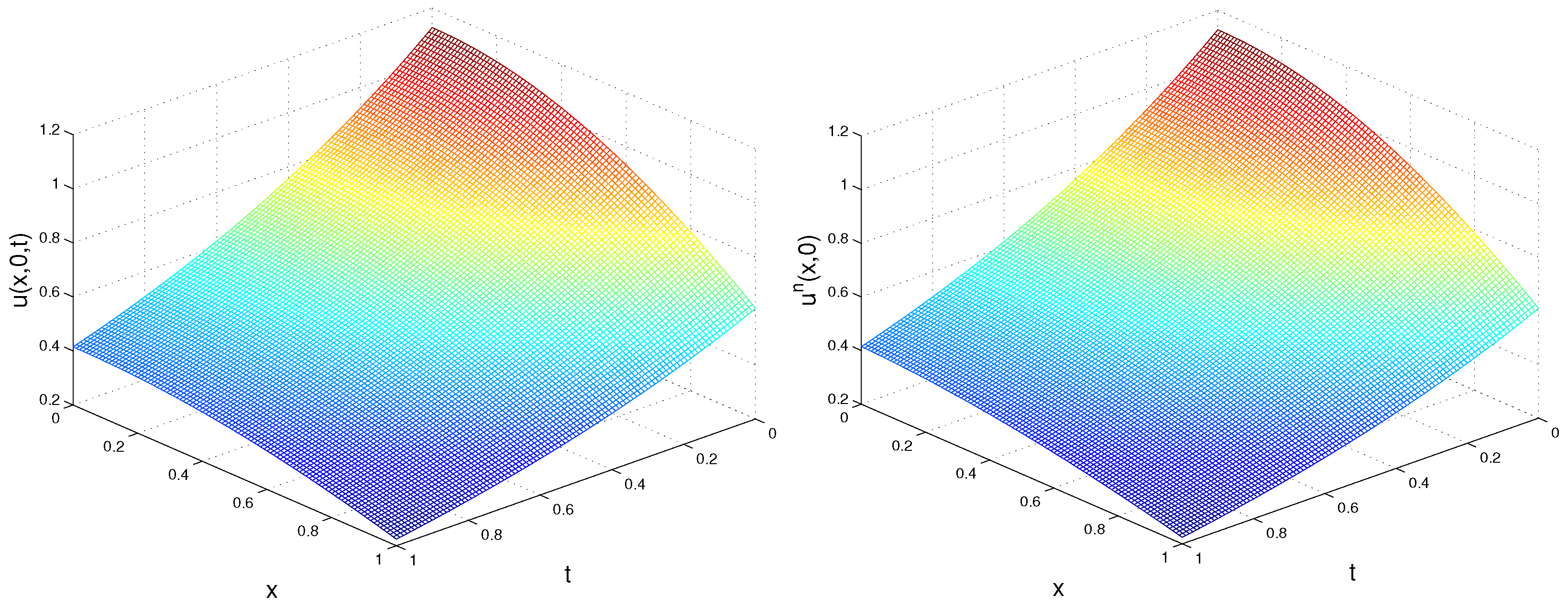
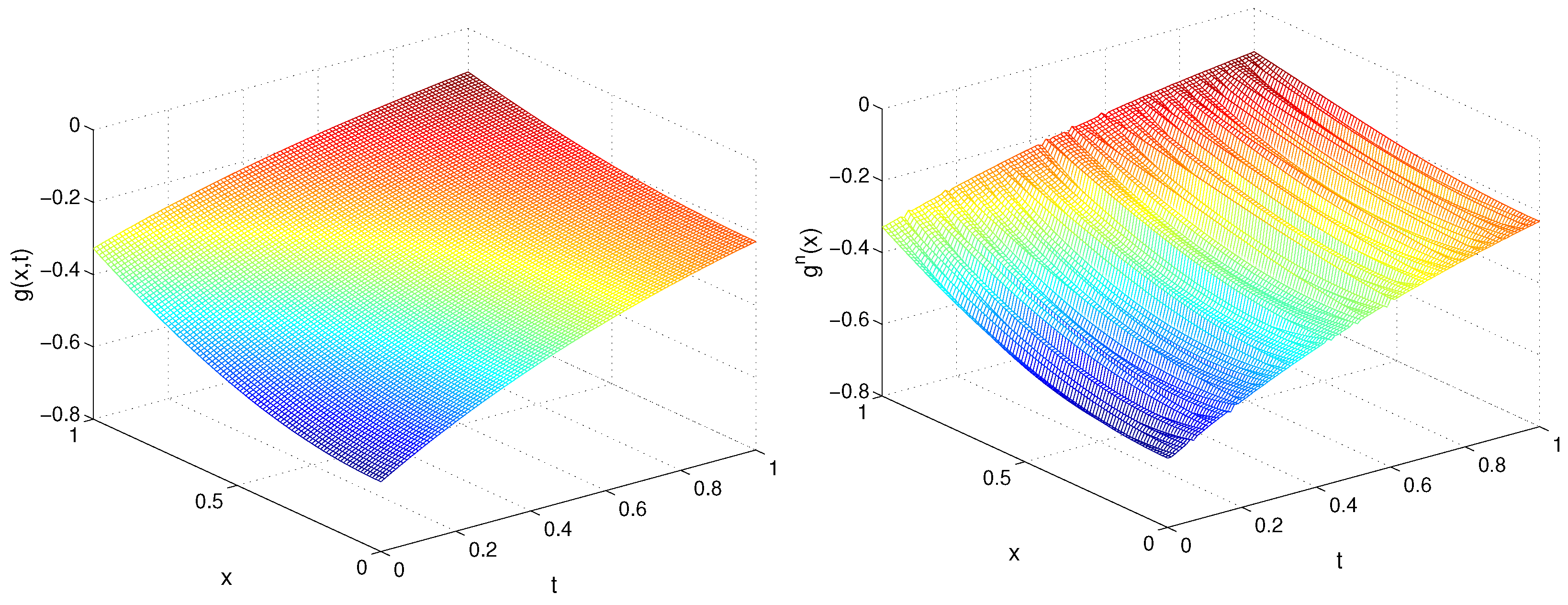
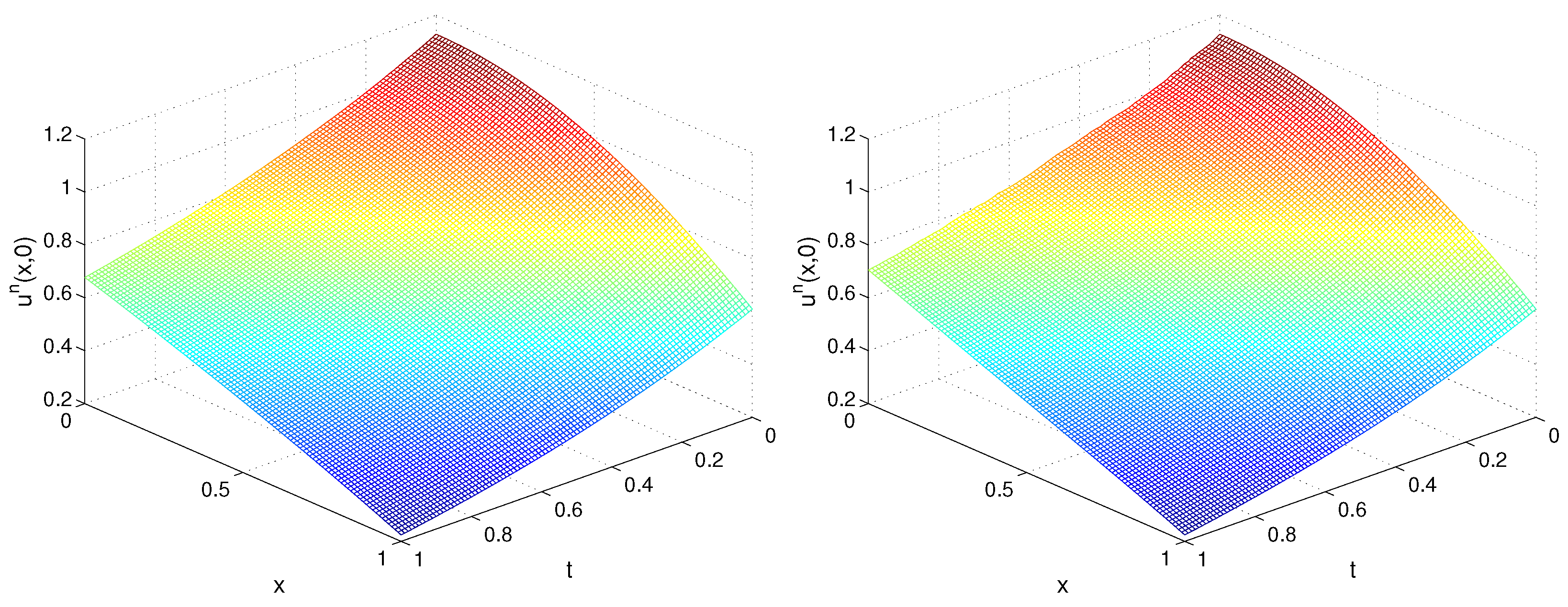
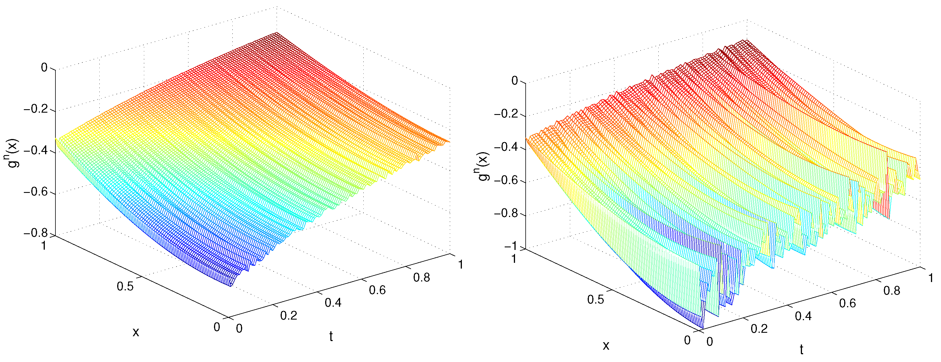
In Figure 1 and Figure 2, we plot the exact and recovered functions $u(x,0,t)$, $g^M\left(x\right)$, respectively, in the $t-x$ plane for TP1, $\rho =0.2$, $m=2$, and $\tau =0.01$.

As was expected, for the lower deviation, we obtained a better accuracy. Moreover, since the exact solution for TP1 only contains the first harmonic term $cos\left(x\right)$, a better accuracy was obtained for $m=1$ and the convergence was very fast in the sense that a small number of iterations were required to obtain optimal accuracy. We observed that, in general, the recovery of the function $u(x,0,t)$ was more precise in comparison with $g(x,t)$ and, independently of the noise level, for a larger m ($m=3$), the precision of the restored source g was better for a smaller time step.

Now, we consider TP2. In

Table 3. Maximum error for different m, time steps, and $\rho =0.2$ for TP2, Example 1.

$\mathit{\tau }$	m	Max. Error ${\mathbf{u}}^{\mathbf{M}}(\mathbf{x},0)$	Max. Error ${\mathbf{g}}^{\mathbf{M}}\left(\mathbf{x}\right)$	Iter
0.01	10	4.3234 $\times {10}^{-2}$	1.9103 $\times {10}^{-1}$	40.763
	15	3.0266 $\times {10}^{-2}$	1.6096 $\times {10}^{-1}$	47.208
	20	2.7671 $\times {10}^{-2}$	1.4172 $\times {10}^{-1}$	51.000
0.005	10	4.2076 $\times {10}^{-2}$	1.8547 $\times {10}^{-1}$	44.582
	15	2.9288 $\times {10}^{-2}$	1.5733 $\times {10}^{-1}$	51.553
	20	2.7508 $\times {10}^{-2}$	1.3997 $\times {10}^{-1}$	60.816

, we present the computational results: the maximum error and average number of iterations for different m, time steps, and noise levels $\rho =0.2$.

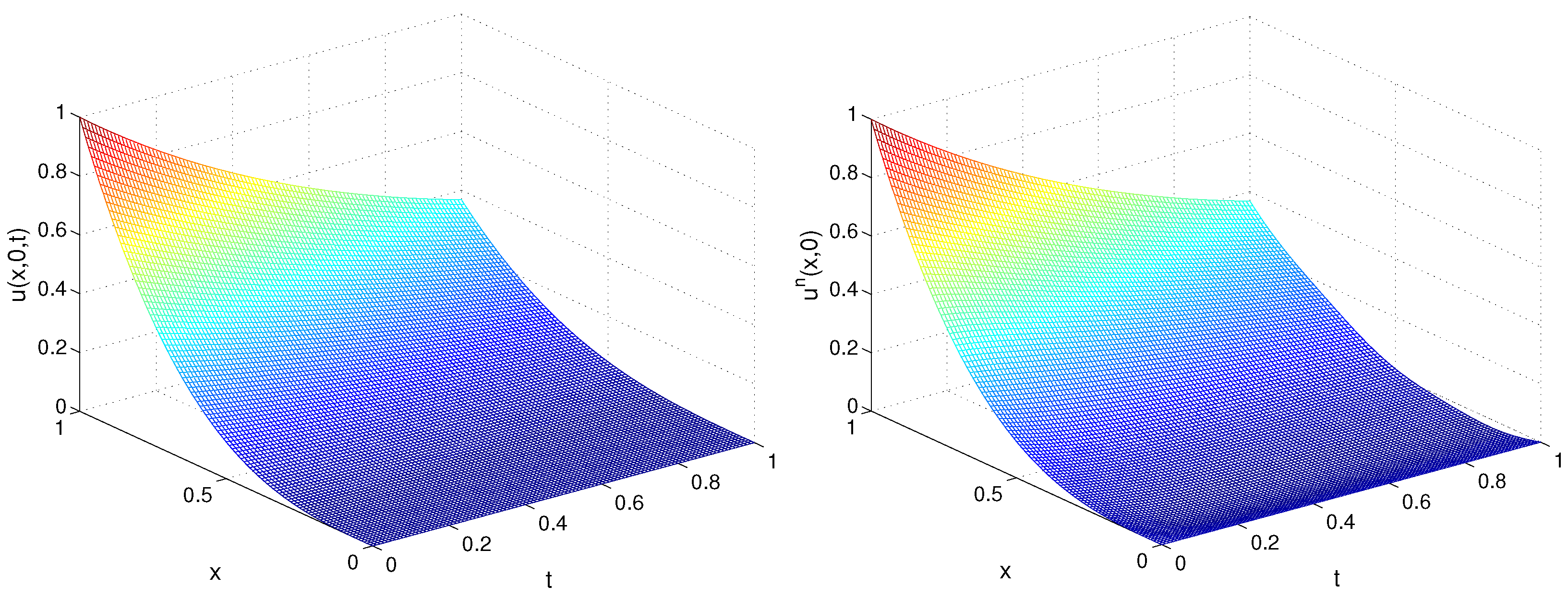
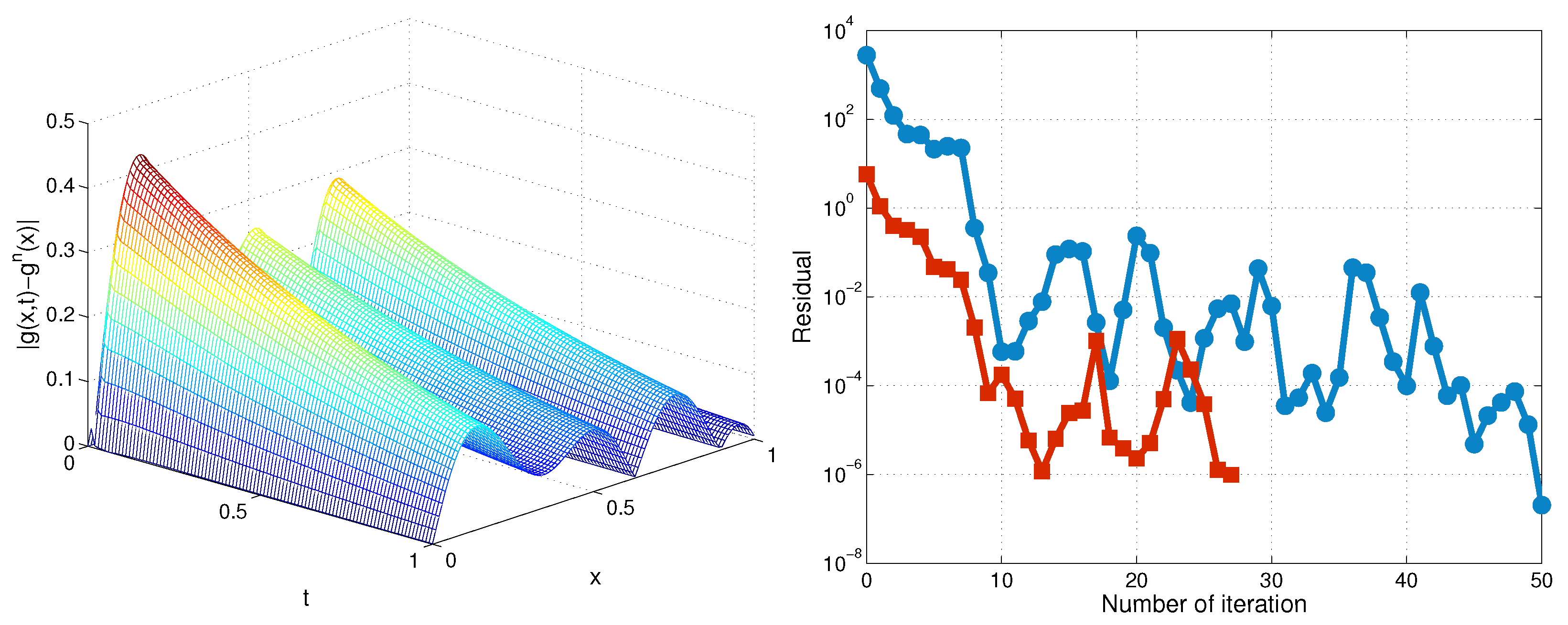
In Figure 3, we depict the exact and recovered function $u(x,0,t)$ for $\rho =0.2$, $m=15$, $\tau =0.01$. In Figure 4, we plot the error $|g(x,t)-g^n\left(x\right)|$ and residual $\parallel r_k\parallel$ at each iteration for $t=\tau$ and $t=T$.

The result shows that as the values of m increased, the accuracy of the recovered functions was affected slightly and the convergence steps increased slightly. Furthermore, the size of the time step did not essentially influence the accuracy.

Example 2. ($\mathbf{IP}-{\mathbf{gu}}_{{\mathsf{\Gamma }}_{\mathbf{0}}}{\mathbf{u}}_{\mathbf{W}}$).  In this example, we tested the efficiency of the proposed algorithm for solving $\mathbf{IP}-{\mathbf{gu}}_{{\mathsf{\Gamma }}_{\mathbf{0}}}{\mathbf{u}}_{\mathbf{W}}$ with perturbed over-determined data (22). The test problems were (1), (6),TP1, and TP2 for $l_1=l_2=1$, $T=1$, and $ϵ=1.e-6$.

In

Table 4. Maximum error for different m and $\rho$, $\tau =0.01$ for TP1, Example 2.

		Max. error	Max. Error	Max. Error
$\rho$	$\mathbf{m}$	${\mathbf{u}}^{\mathbf{M}}(\mathbf{x},\mathbf{0})$	${\mathbf{g}}^{\mathbf{M}}\left(\mathbf{x}\right)$	${\mathbf{u}}_{\mathbf{W}}^{\mathbf{M}}\left(\mathbf{y}\right)$	Iter
0.02	1	1.8693 $\times {10}^{-2}$	4.2198 $\times {10}^{-3}$	1.9027 $\times {10}^{-1}$	13.821
	2	2.6226 $\times {10}^{-1}$	3.7340 $\times {10}^{-2}$	2.8543 $\times {10}^{-1}$	15.772
	3	2.4577 $\times {10}^{-1}$	8.0663 $\times {10}^{-2}$	2.8665 $\times {10}^{-1}$	19.841
0.2	1	5.8913 $\times {10}^{-2}$	6.2845 $\times {10}^{-2}$	2.6709 $\times {10}^{-1}$	13.862
	2	2.3012 $\times {10}^{-1}$	2.4847 $\times {10}^{-1}$	1.5154 $\times {10}^{-1}$	15.861
	3	2.1429 $\times {10}^{-1}$	6.2469 $\times {10}^{-1}$	2.1894 $\times {10}^{-1}$	19.594

, we present the maximal errors and average number of iterations of the recovered functions at the final time for TP1 with different noise levels and $\tau =0.01$.

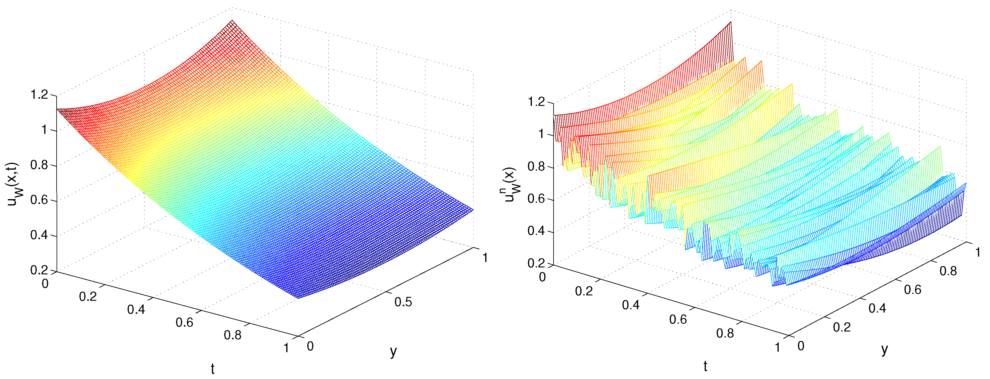
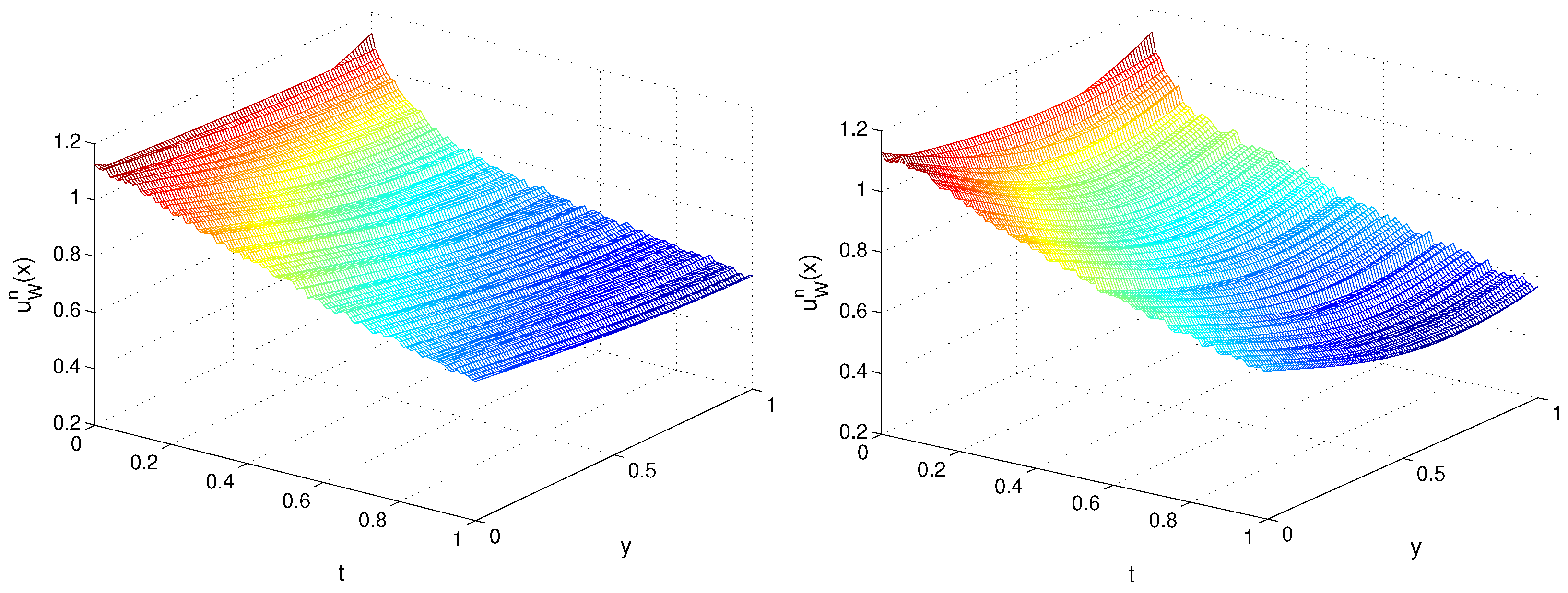
In Figure 5 and Figure 6, we plot the recovered functions $u^n(x,0)$ and $g^n\left(x\right)$ for TP1, $m=2$, $\tau =0.01$, $\rho =0.02$, and $\rho =0.2$. Next, in Figure 7 and Figure 8, on the $y-t$ plane, we depict the exact $u_W(y,t_n)$ and recovered boundary condition $u_W^n\left(y\right)$ for TP1, $\tau =0.01$, and different values of $\rho$ and m.

In

Table 5. Maximum error for $\rho =0.2$, $\tau =0.01$ and different m for TP2, Example 2.

	Max. Error	Max. Error	Max. Error
$\mathbf{m}$	${\mathbf{u}}^{\mathbf{M}}(\mathbf{x},\mathbf{0})$	${\mathbf{g}}^{\mathbf{M}}\left(\mathbf{x}\right)$	${\mathbf{u}}_{\mathbf{W}}^{\mathbf{M}}\left(\mathbf{y}\right)$	Iter
10	1.7842 $\times {10}^{-1}$	1.6864 $\times {10}^{-1}$	2.5069 $\times {10}^{-1}$	39.267
15	1.4291 $\times {10}^{-1}$	1.4003 $\times {10}^{-1}$	1.1296 $\times {10}^{-1}$	41.733
20	1.2674 $\times {10}^{-1}$	1.4083 $\times {10}^{-1}$	1.9546 $\times {10}^{-1}$	48.831

, we present the computational results for TP2.

We observed that the function $u^n(x,0)$ exhibited a higher accuracy than $u^n\left(x\right)$ and $u_W^n\left(y\right)$. The level of noise influenced the accuracy of the recovered functions, while the values of m did not affect it significantly. As for $\mathbf{IP}-{\mathbf{gu}}_{{\mathsf{\Gamma }}_{\mathbf{0}}}$, we observed a slight increase in the convergence steps.

6. Discussion

The proposed method is able to simultaneously recover two or three space–time-dependent functions (Dirichlet boundary conditions and the source term in the dynamical boundary condition) in the initial boundary value problem for Laplace’s equation with dynamical boundary conditions. The temporal order of the convergence of the solution for exact measurements is first for the Dirichlet boundary and second for the source term. As is typical for solutions of inverse problems with perturbed data, the order of convergence is destroyed, i.e., it becomes lower as the deviation increases.

The method introduced is a comprehensive approach in which Trefftz-type test functions are directly incorporated into Green’s second identity to formulate a linear system for reconstructing unknown data using a finite Fourier series. This approach eliminates the necessity of regularization techniques and is robust enough to handle significant levels of noise. For example, we achieved optimal accuracy and relevant results for a moderate number of iterations. In contrast, in the other methods in the literature for solving inverse Cauchy problems, for example, those using the modified collocation Trefftz method (see, e.g., [48,49]), the authors employ regularization techniques by truncating the higher modes of the Fourier series of the input data or using a scaling factor in the Trefftz functions.

The considered inverse problem can be solved using a boundary-type solution procedure. In our paper, the global relation (13) is derived using the second Green identity so that the input data generation is much easier than when using domain-type algorithms.

The weakness of the approach is that, in contrast to some iteration-free approaches (see, e.g., [38]), we use an iteration procedure, which requires additional computational time. Furthermore, it is essential to select a value for m within a moderate range, as an excessively large m could results in an inaccurate outcome.

Although, in general, the Trefftz method is of high precision, the presented approach involves an approximation in time, which generates a discretization error. Furthermore, additional errors arise from the noise in the input data.

The limitations of the proposed numerical approach are related to the fact that it uses the smoothness of solution. Additionally, for elliptic equations with non-constant coefficients, it is difficult to further develop the method.

7. Conclusions

The reconstruction of the dynamical boundary condition source and Dirichlet boundary condition from Dirichlet–Neumann measurements for Laplace’s equation was investigated. In the first stage of our study, we performed time semi-discretization for the problem. Then, applying Green’s second identity to the Laplace boundary value problem, we constructed an integral equation, which connects the source of the dynamical boundary condition and the Dirichlet and Neumann boundary conditions. By successfully picking the Trefftz test function, we developed an algorithm to numerically establish the dynamical and Dirichlet boundary conditions.

The numerical results show that the suggested method is stable and efficient for strongly ill-posed cases with a large amount of noise imposed on the over-specified boundary data. The noise level has a greater impact on the accuracy of the recovered space–time-dependent boundary functions as compared to the time mesh step size.

Our future work will investigate the theoretical convergence of the proposed numerical method. Furthermore, we plan to study inverse problems for elliptic equations with semi-linear dynamical boundary conditions like the problem investigated in Section 6 of [5,44].

References

- Crank, J. The Mathematics of Diffusion; Clarendon Press: Oxford, UK, 1973. [Google Scholar]
- Gröger, K. Initial boundary value problems from semiconductor device theory. Z. Angew. Math. Mech. 1978, 67, 345–355. [Google Scholar] [CrossRef]
- Langer, R.E. A problem in diffusion or in the flow of heat for a solid in contact with a fluid. Tohoka Math. J. 1972, 35, 260–275. [Google Scholar]
- Fila, M.; Quittner, P. Global solutions of the Laplace equation with a nonlinear dynamical boundary condition. Math. Appl. Sci. 1997, 20, 1325–1333. [Google Scholar] [CrossRef]
- Koleva, M.N.; Vulkov, L.G. Blow-up of continuous and semilinear solutions to elliptic equations with semilinear dynamical boundary conditions of parabolic type. J. Comp. Appl. Math. 2007, 202, 414–434. [Google Scholar] [CrossRef]
- Jovanovic, B.S.; Vulkov, L.G. Convergence of difference schemes for the Poisson equation dynamical interface conditions. Comput. Methods Appl. Math. 2003, 3, 177–188. [Google Scholar] [CrossRef]
- Jovanovic, B.S.; Vulkov, L.G. Convergence of finite difference schemes for the Poisson’s equation with a dynamic boundary condition. Comput. Methods Appl. Math. 2005, 45, 275–284. [Google Scholar]
- Vabishchevich, P.N. Numerical solution of a problem for the elliptic equation with unsteady boundary conditions. Matem Model. 1995, 7, 49–60. (In Russian) [Google Scholar]
- Isakov, V. Inverse Source Problems; AMS: Providence, RI, USA, 1989. [Google Scholar]
- Grysa, K.; Macia̧g, A. Identifying heat source intensity in treatment of cancerous tumor using therapy based on local hyperthermia—The Trefftz method approachs. J. Therm. Biol. 2019, 84, 16–25. [Google Scholar] [CrossRef]
- Hasanoglu, A.; Romanov, V.G. Introduction to Inverse Problems for Differential Equations, 1st ed.; Springer: Cham, Switzerland, 2017; 261p. [Google Scholar]
- Kabanikhin, S.I. Inverse and Ill-Posed Problems; DeGruyer: Berlin, Germany, 2011. [Google Scholar]
- Lesnic, D. Inverse Problems with Applications in Science and Engineering; CRC Pres: Abingdon, UK, 2021; p. 349. [Google Scholar]
- Samarskii, A.A.; Vabishchevich, P.N. Numerical Methods for Solving Inverse Problems in Mathematical Physics; de Gruyter: Berlin, Germany, 2007; 438p. [Google Scholar]
- Ait Ben Hassi, E.M.; Chorfi, S.-E.; Maniar, L. Identification of source terms in heat equation with dynamic boundary conditions. Math. Meth. Appl. Sci. 2022, 45, 2364–2379. [Google Scholar] [CrossRef]
- Ivanov, D.K.; Kolesov, A.E.; Vabischevich, P.N. Numerical method for recovering the piecewise constant right-hand side function of an alliptic equation from a partial boundary observation data. J. Phys. Conf. Ser. 2021, 2092, 012006. [Google Scholar] [CrossRef]
- Liu, C.-S. A BIEM using the Treftz test functions for solving the inverse Cauchy and source recovery problems. Engn. Anal. Bound. Elem. 2016, 62, 177–185. [Google Scholar] [CrossRef]
- Liu, C.-S.; Cheng, C.-W. A global boundary integral equation method for recovering space-time dependent heat source. Int. J. Heat Mass Transf. 2016, 92, 1034–1040. [Google Scholar] [CrossRef]
- Yu, W. Well-posednes of determining the source term of elliptic equation. Bull. Austral. Math. Soc. 1994, 50, 383–398. [Google Scholar] [CrossRef]
- Tikhonov, A.N.; Goncharsky, A.V.; Stepanov, V.V.; Yagola, A.G. Numerical Methods for the Solution of Ill-Posed Problems, 1st ed.; Springer: Dordrecht, The Netherlands, 1995; 253p. [Google Scholar]
- Tikhonov, A.N.; Arsenin, V.Y. Solutions of Ill-Posed Problems; V. H. Winston & Sons: Washington, DC, USA; John Wiley & Sons: New York, NY, USA, 1977; 258p, (Translated from Russian). [Google Scholar]
- Belgacem, F.B. Why is the Cauchy problem severely ill-posed? Inverse Probl. 2007, 23, 823–836. [Google Scholar] [CrossRef]
- Cheng, J.; Hon, Y.C.; Wei, T.; Yamamoto, M. Numerical computation of a Cauchy problem for Laplace’s equation. Z. Angew. Math. Mech. 2001, 81, 665–674. [Google Scholar] [CrossRef]
- Joachimiak, M.; Ciałkowski, M.; Fra̧ckowiak, A. Stable method for solving the Cauchy problem with the use of Chebyshev polynomials. Int. J. Numer. Methods Heat Fluid Flow 2019, 30, 1441–1456. [Google Scholar] [CrossRef]
- Joachimiak, M.; Joachimiak, D.; Ciałkowski, M. Investigation on thermal loads in steady-state conditions with the use of the solution to the inverse problem. Heat Transf. Eng. 2023, 44, 963–969. [Google Scholar] [CrossRef]
- El Hajji, M.; Jday, F. Boundary data completion for a diffusion-reaction equation based on the minimization of an energy error functional using conjugate gradient method. Punjab Univ. J. Math. 2019, 51, 25–43. [Google Scholar]
- Kirkeby, A. Feynman’s inverse problem. arXiv 2023. [Google Scholar] [CrossRef]
- Alessandrini, G. A small collection of open problems. Rend. Istit. Mat. Univ. Trieste 2020, 52, 591–600. [Google Scholar]
- Rundell, R. Some inverse problems for elliptic equations. Appl. Anal. Int. J. 1988, 28, 67–78. [Google Scholar] [CrossRef]
- Slodička, M.; Lesnic, D. Determination of the Robin coefficient in a nonlinear boundary condition for a steady-state problem. Math. Meth. Appl. Sci. 2009, 32, 1311–1324. [Google Scholar] [CrossRef]
- Engl, H.W.; Leitão, A. A Mann iterative regularization method for elliptic Cauchy problems. Numer. Funct. Anal. Optim. 2001, 22, 861–884. [Google Scholar] [CrossRef]
- Kozlov, V.A.E.; Maz’ya, V.G.; Fomin, A.V. An iterative method for solving the Cauchy problem for elliptic equation. Comput. Math. Phys. 1991, 31, 45–52. [Google Scholar]
- Gong, R.; Wang, M.; Huang, Q.; Zhang, Y. Inverse Cauchy problems: Revisit and a new approach. arXiv 2022. [Google Scholar] [CrossRef]
- Jaoua, M.; Chaabane, S.; Elhechmi, C.; Leblond, J.; Mahjoub, M.; Partington, J. On some robust algorithms for Robin inverse problem. Rev. Arima 2008, 9, 287–307. [Google Scholar]
- Shirzadi, A.; Takhtabnoos, F. A local meshless method for Cauchy problem of elliptic PDEs in annulus domains. Inverse Probl. Sci. Eng. 2016, 24, 729–743. [Google Scholar] [CrossRef]
- Liu, C.-S.; Wang, F. A meshless method for solving the nonlinear inverse Cauchy problem of elliptic type equation in a doubly-connected domain. Comput. Math. Appl. 2018, 76, 1837–1852. [Google Scholar] [CrossRef]
- Wang, L.; Qian, Z.; Wang, Z.; Gao, Y.; Peng, Y. An efficient radial basis collocation method for the boundary condition identification of the inverse wave problem. Int. J. Appl. Mech. 2018, 10, 1850010. [Google Scholar] [CrossRef]
- Wang, L.; Wang, Z.; Qian, Z. A meshfree method for inverse wave propagation using collocation and radial basis functions. Comput. Methods Appl. Mech. Engrg. 2017, 322, 311–350. [Google Scholar]
- Hu, M.; Wang, L.; Yang, F.; Zhou, Y. Weighted radial basis collocation method for the nonlinear inverse Helmholtz problems. Mathematics 2023, 11, 662. [Google Scholar] [CrossRef]
- Ciałkowski, M.; Olejnik, A.; Joachimiak, M.; Grysa, K.; Fra̧ckowiak, A. Cauchy type nonlinear inverse problem in a two-layer area. Int. J. Numer. Methods Heat Fluid Flow 2021, 32, 313–331. [Google Scholar] [CrossRef]
- Karageorghis, A.; Lesnic, D.; Marin, L. A survey of applications of the MFS to inverse problems. Inverse Probl. Sci. Eng. 2011, 19, 309–336. [Google Scholar] [CrossRef]
- Liu, C.-S.; Qu, W.; Zhang, Y. Numerically solving twofold ill-posed inverse problems of heat equation by the adjoint Trefftz method. Numer. Heat Transf. Part B 2018, 73, 48–61. [Google Scholar] [CrossRef]
- Chorfi, S.E.; El Guermai, G.; Maniar, L.; Zouhair, W. Numerical identification of initial temperatures in heat equation with dynamic boundary conditions. Mediterr. J. Math. 2023, 20, 256. [Google Scholar] [CrossRef]
- Constantin, A.; Escher, J. Global solutions for quasilinear parabolic problems. J. Evol. Equations 2002, 2, 97–111. [Google Scholar] [CrossRef]
- Craig, W. A Course on Partial Differential Equations. Amer. Math. Soc. 2018, 197, 205. [Google Scholar]
- Esher, J. Smooth solutions of nonlinear elliptic systems with dynamic boundary conditions. In: Evolution equations, control theory, and biomathematics (Han sur Lesse, 1991). Lect. Notes Pure Appl. Math. 1994, 155, 173–183. [Google Scholar]
- Yin, Z. Global existence for elliptic equations with dynamic boundary conditions. Arch. Math. 2003, 81, 567–574. [Google Scholar] [CrossRef]
- Liu, C.-S. A highly accurate MCTM for inverse Cauchy problems of Laplace equation in arbitrary plane domains. Comput. Model. Eng. Sci. 2008, 35, 91–111. [Google Scholar]
- Liu, C.-S. A modified collocation Trefftz method for the inverse Cauchy problem of Laplace equation. Eng. Anal. Bound. Elem. 2008, 32, 778–785. [Google Scholar] [CrossRef]
Figure 1.
Exact (left) and recovered (right) function for TP1, Example 1.
Figure 2.
Figure 3.
Exact (left) and recovered (right) function for TP2, Example 1.
Figure 4.
Error in plane (left) and residual vs. the iteration number (right) for (line with circles) and (line with squares) for TP2, Example 1.
Figure 5.
Recovered function for TP1, , (left) and (right) for Example 2.
Figure 6.
Figure 7.
Exact (left) and recovered (right) function , , for TP1, Example 2.
Figure 8.
Recovered function , , (left) and (right) for TP1, Example 2.