Article

A Novel Fractional Multi-Order High-Gain Observer Design to Estimate Temperature in a Heat Exchange Process

by
Vicente Borja-Jaimes
1,
Manuel Adam-Medina
1,
Jarniel García-Morales
1,
Alan Cruz-Rojas
2,
Alfredo Gil-Velasco
3 and
Antonio Coronel-Escamilla
4,*
1
Departamento de Ingeniería Electrónica, TecNM-Centro Nacional de Investigación y Desarrollo Tecnológico (CENIDET), Cuernavaca 62490, Morelos, Mexico
2
Departamento de Ciencias Computacionales e Ingenierías, Centro Universitario de los Valles, Universidad de Guadalajara, Ameca 46600, Jalisco, Mexico
3
Dirección Académica de la Ingeniería en Tecnologías de la Información y la Ingeniería en Electrónica y Telecomunicaciones, Universidad Politécnica del Estado de Morelos, Jiutepec 62550, Morelos, Mexico
4
División Académica de Mecánica Industrial, Universidad Tecnológica Emiliano Zapata del Estado de Morelos, Emiliano Zapata 62765, Morelos, Mexico
*
Author to whom correspondence should be addressed.
Axioms 2023, 12(12), 1107; https://doi.org/10.3390/axioms12121107
Submission received: 16 October 2023 / Revised: 23 November 2023 / Accepted: 30 November 2023 / Published: 8 December 2023
(This article belongs to the Special Issue Fractional Calculus: From Fundamentals to Modern Applications)

Abstract

:
In the present manuscript, we design a fractional multi-order high-gain observer to estimate temperature in a double pipe heat exchange process. For comparison purposes and since we want to prove that when using our novel technique, the estimation is more robust than the classical approach, we design a non-fractional high-gain observer, and then we compare the performance of both observers. We consider three scenarios: The first one considers the estimation of the system states by measuring only one output with no noise added on it and under ideal conditions. Second, we add noise to the measured output and then reconstruct the system states, and, third, in addition to the noise, we increase the gain parameter in both observers (non-fractional and fractional) due to the fact that we want to prove that the robustness changes in this parameter. The results showed that, using our approach, the estimated states can be recovered under noise circumstances in the measured output and under parameter change in the observer, contrary to using classical (non-fractional) observers where the states cannot be recovered. In all our tests, we used the normalized root-mean-square, integral square error, and integral absolute error indices, resulting in a better performance for our approach than that obtained using the classical approach. We concluded that our fractional multi-order high-gain observer is more robust to input noise than the classical high-gain observer.

1. Introduction

Nowadays, heat exchangers find extensive utilization across diverse industrial and engineering applications. Heat exchangers are devices designed to efficiently transfer heat from one fluid to another without the fluids coming into direct contact [1]. A special kind of heat exchanger called a double pipe heat exchanger (DPHE) has attracted significant attention from researchers, engineers, and industries due to several advantages, such as compact design, versatility, flexibility, modularity, easy cleaning and maintenance, and cost-effectiveness [2]. DPHEs are commonly used for applications with low-to-medium heat transfer requirements, such as small-scale heating and cooling systems, laboratory experiments, and industrial processes. Due to their wide-ranging applications, extensive research on DPHEs has been conducted, with a primary focus on enhancing their efficiency and performance [3]. In order to enhance the performance and efficiency of DPHEs, monitoring and control systems are integrated.
Monitoring systems play a pivotal role by measuring various variables in DPHEs, significantly contributing to the optimization of efficiency, maintenance of stability, assurance of safety, and enhancement of adaptability to changing conditions [4]. Although monitoring systems provide several advantages, sometimes it is impractical to use them due to factors such as cost, accuracy, hardware sensor availability, issues related to signal interference, and measurement noise [5]. The presence of measurement noise in a monitoring system may result in diverse consequences, including inaccuracies in measurements [6], heightened uncertainty, and the occurrence of faults [7,8]. Furthermore, in the context of a closed-loop control system, the presence of measurement noise can significantly affect its performance. This noise has the potential to introduce fluctuations in the feedback signals utilized by the controller, consequently resulting in suboptimal or erratic control performance [9]. To mitigate the effects of measurement noise in monitoring systems, several techniques have been used, such as filtering algorithms [10], signal processing methods [11], and software sensors [12]. Software sensors, commonly referred to as observers (or virtual sensors), have emerged as a viable substitute for addressing the issue of measurement noise and the unavailability of hardware sensors due to system configuration or cost. Different observers have been used to estimate (predict) both state variables and parameters in DPHEs from online or offline measurements [13]. Intelligent observers for performing estimation on heat exchangers using fuzzy logic, genetic algorithms, and artificial neural networks (ANNs) have been proposed in the literature [14]. In [15], the authors introduce a simple method to predict the cold and hot fluid outlet temperatures in a counter-flow DPHE using fuzzy logic. The nonlinear nature of the DPHE has given rise to nonlinear observers, such as extended Kalman filters [16], sliding mode observers [17], and high-gain observers [18]. High-gain observers (HGOs) have become a significant focus in the fields of state estimation and output feedback control for nonlinear systems. In the absence of measurement noise, these observers robustly estimate the states of the DPHEs, ensuring fast convergence [19]. Nevertheless, the HGO theory reveals a tradeoff between measurement noise sensitivity and the speed of convergence in estimation. As the HGO gain increases, its bandwidth expands. Consequently, with the escalating bandwidth, the HGO asymptotically approximates the characteristics of a differentiator, amplifying the impact of measurement noise [20]. As fast convergence is crucial in observer implementations, increased observer gain is necessary; consequently, addressing the issue of noise sensitivity becomes imperative.
On the other hand, there is a mathematical area called fractional-order calculus (FOC) which has been gaining attention in recent years because it deals with derivatives and integrals of non-integer order [21]. FOC has been widely used to describe the behavior of different systems in applications such as electrical engineering, chemical engineering, control engineering, bioengineering, neuroscience, and so on [22,23]. The increasing interest in FOC in dynamical systems is because it has been demonstrated that FOC can model system properties that are intrinsically related to non-local behavior, such as the memory effect [24]. These kinds of systems are also called non-Markov systems. Moreover, several authors have demonstrated the effectiveness of FOC in the estimation of signals in applications such as the design of fractional-order observers (FO-observers) [25,26,27] and fractional-order controllers [28,29,30]. Some authors have proposed fractional-order high-gain observers (FO-HGOs) to estimate system states, design controllers, synchronize systems, signal processing, monitoring, and so on [31,32]. However, the study of fractional multi-orders in an HGO has not been reported in the literature; some authors have studied the behavior of fractional differential systems with multi-orders [33,34], along with the numerical approximation of such systems [35]. We use previous results to extend the use of fractional multi-order systems to the design of a high-gain observer. The utilization of a fractional multi-order high-gain observer (FMO-HGO) in our study is considered a novel approach for two principal reasons. Firstly, it introduces the concept of fractional multi-order calculus, enabling the more accurate modeling of non-integer order dynamics. Secondly, the FMO-HGO exhibits reduced sensitivity to noise compared to the classical (non-fractional) HGO, thereby enhancing the robustness and accuracy of state estimation, particularly in the presence of measurement noise.
To validate the efficacy of the proposed FMO-HGO, we conducted an experimental configuration using a DPHE pilot plant RCT 100 operating in an open-loop system. The experiment is focused on estimating the outlet temperatures with both integer and fractional-order observers, utilizing measurements of both inlet and outlet temperatures. To demonstrate the effectiveness of the proposed observer in reducing noise sensitivity, we explored two scenarios, considering experimental data with noise and variations in the observer’s gain. For the evaluation of the proposed FMO-HGO’s performance, we utilized the integral square error (ISE) and integral absolute error (IAE) indices, along with the normalized root-mean-square error (NRMSE) criterion.
The remainder of this manuscript is organized as follows. Section 2 presents the fractional calculus definitions used in this work and the numerical algorithm used to solve fractional-order differential equations. Section 3 describes the mathematical model of the DPHE, and in Section 4 we present the development of the HGO and the FMO-HGO along with the numerical solution for the FMO-HGO. In Section 5, we present the results of this research. Finally, Section 6 shows the discussions and conclusions of this manuscript.

2. Fractional Calculus Definitions

Three of the most important definitions in fractional-order calculus (FOC) are the Riemann–Liouville (RL), Grunwald–Letnikov (GL), and Caputo definitions [36]. These definitions have been extended and used in several applications such as modeling, control, and signal processing [37]. We first present the RL definition of a fractional-order integral.
Let f :   [ 0 , ) be a continuous function. Then, the fractional RL integral definition is formulated as
I 0 RL t β f ( t ) = 1 Γ ( β ) d m d t m 0 t f ( η ) ( t η ) β 1 d η ,   t > 0
where β > 0 is the fractional-order in the integral and it can be any real number, that is, β , Γ ( · ) denotes the Gamma function and it is defined as
Γ ( z ) = 0 t z 1 exp ( t ) d t
Note that, if β takes the value of one, then the RL integral is equal to the classical integral definition. Now, assuming the same conditions for function f ( t ) , the fractional RL derivative of order α , with α > 0 and m = [ α ] + 1 , is defined as
D 0 RL t α f ( t ) = 1 Γ ( m α ) d m d t m 0 t f ( η ) ( t η ) m α 1 d η ,   t > 0
note that, when α = 1 , then the RL derivative is equal to the classical derivative definition.
Finally, we define the Caputo derivative of order α as
D 0 C t α f ( t ) = 1 Γ ( m α ) 0 t f ( m ) ( η ) ( t η ) m α 1 d η ,   t > 0
For the Caputo derivative, we have that when α = 1 , we recover the classical derivative definition.

Numerical Algorithms to Solve Fractional-Order Differential Equations

Solving a fractional-order differential equation can be difficult in most cases. However, there are several numerical methods to solve these kinds of equations. In this work, we use the Grunwald–Letnikov (GL) algorithm. This numerical method is based on the GL derivative, and it allows us to compute a numerical solution of fractional-order differential equations. The GL algorithm is particularly useful when dealing with both RL and Caputo derivatives. This algorithm has been widely employed for the numerical solution of fractional-order differential equations, and several works have demonstrated its robustness and performance [38].
The GL definition is formulated from the GL derivative, which is defined as follows
D 0 GL t q f ( t ) = lim h 0 1 h q j = 0 t / h ( 1 ) j ( q j ) f ( t j h )
where q is the order in the derivative and q     , j denotes the time increment. Note that, in the first case when q   [ 1 , 0 ) , this is considered the fractional-order integral and q   ( 0 , 1 ] is the fractional-order derivative; evidently, if q = 0 , this means there is an algebraic relation, thus no dynamics are presented. For the calculation of the binomial coefficients, we use the relation between Euler’s Gamma function and factorial, that is
( q j ) = Γ ( q + 1 ) Γ ( j + 1 ) Γ ( q j + 1 )
The GL definition allows to calculate the numerical solution of a fractional-order differential equation as follows
D 0 GL t q f ( t ) = g ( f ( t ) )
The numerical solution is expressed as [39]
f ( t k ) = g ( f ( t k 1 ) ) h q j = 1 k c j q f ( t k j )
c j q = ( 1 1 + q j ) c j 1 q
where h is the time step, the initial coefficient value is set to c 0 q = q , and the summation part of the numerical solution is called the intrinsic memory trace.

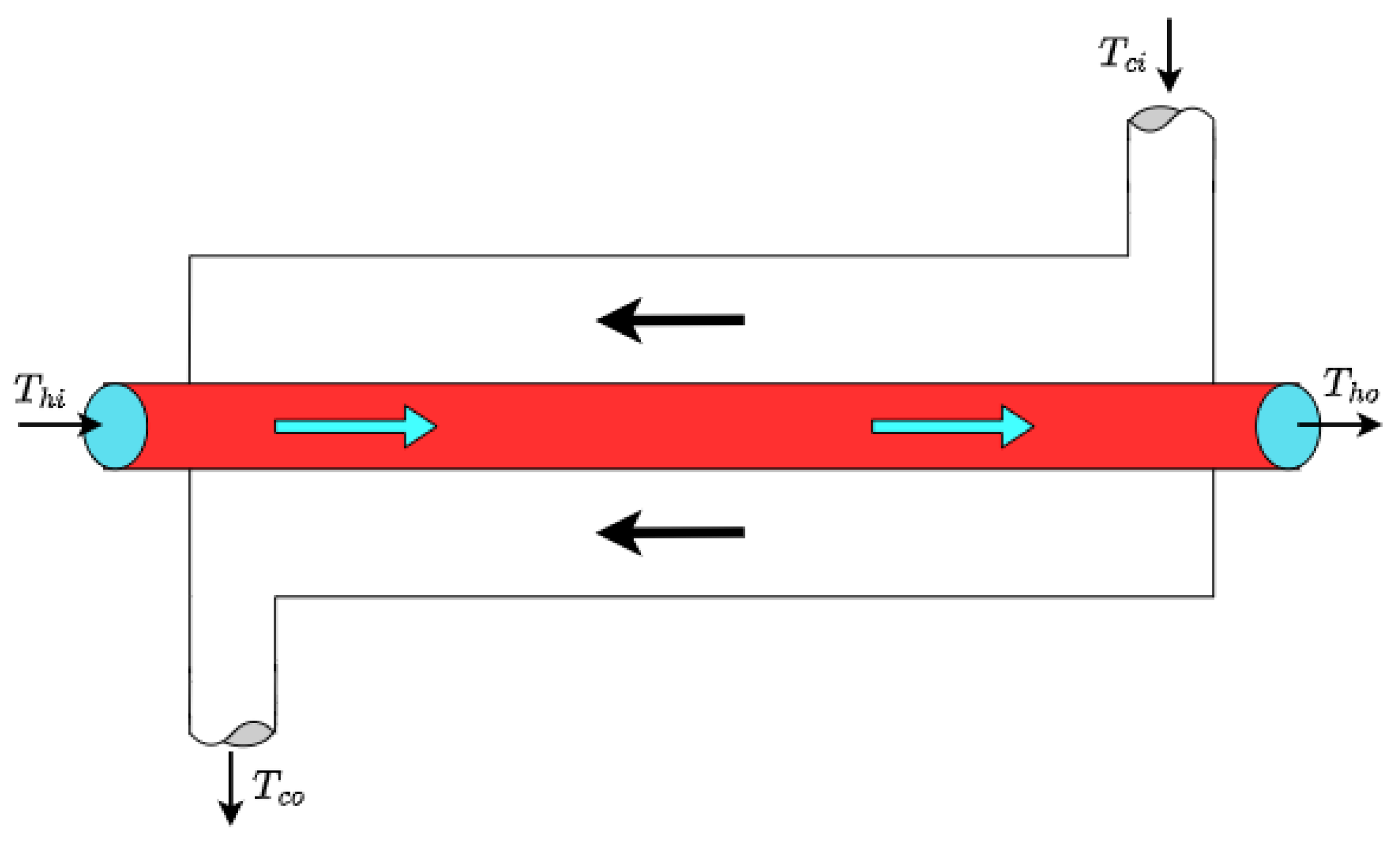
3. Mathematical Model of a Double Pipe Heat Exchanger (DPHE)

A heat exchanger is a device that facilitates the transfer of heat from one fluid to another. Heat exchangers are commonly used in various industrial processes such as power generation, oil refining, chemical processing, refrigeration, and air conditioning. Heat exchangers play a crucial role in improving energy efficiency, reducing operational costs, and controlling temperature in various processes by efficiently transferring heat between different fluids [40].
The basic structure of a heat exchanger consists of two main channels or passages for hot and cold fluids. These channels can be arranged in various ways, such as parallel-flow, counterflow, or crossflow configurations. The dividing wall between the two channels is typically made of a thermally conductive material, such as metal [41].
As we mentioned earlier, in this paper we focus on a special type of heat exchanger known as a double pipe heat exchanger (DPHE) or concentric tube heat exchanger. DPHEs are relatively simple in design and construction, making them cost-effective and easy to maintain. DPHEs find applications in various industries where heat transfer between two fluids is required, such as the chemical industry, pharmaceutical industry, oil and gas industry, etc. [42].
A DPHE is formed by two pipes or tubes arranged in a concentric manner, as shown in Figure 1. The inner tube carries the hot fluid, while the outer tube carries the cold fluid. The two fluids flow in a counter-flow or parallel-flow arrangement depending on the design. The counter-flow configuration of heat exchangers offers several advantages, like a more efficient heat transfer rate per unit surface area, reduced thermal stress, and flexibility in fluid compatibility, making it a preferred choice in many industrial and commercial applications [43].
The mathematical model of the DPHE is derived based on the following assumptions:
  • The thermophysical properties of the fluids are constant.
  • The overall heat transfer coefficient remains constant and uniform along the axial direction.
  • The process is adiabatic, meaning there is no heat exchange with the surrounding environment.
  • The fluids are incompressible and monophasic.
  • The walls do not store energy.
  • The volume in the tubes is constant.
Based on the above assumptions and by applying an energy balance law to the DPHE cell, the lumped parameter representation of the DPHE model is as follows:
T ˙ c o ( t ) = 2 V c [ U A c c p c ρ c Δ T ( t ) + ( T c i ( t ) T c o ( t ) ) v c ( t ) ] , T ˙ h o ( t ) = 2 V h [ U A h c p h ρ h Δ T ( t ) + ( T h i ( t ) T h o ( t ) ) v h ( t ) ] .
The variables and parameters of the model in Equation (10) are described in Table 1. Δ T ( t ) represents the logarithmic mean temperature difference (LMTD), which is a function of both outlet temperatures, T c o ( t ) and T h o ( t ) . The LMDT among the fluids is commonly expressed as
Δ T ( t ) = Δ T 2 ( t ) Δ T 1 ( t ) ln ( Δ T 2 ( t ) / Δ T 1 ( t ) ) .
The temperature difference between each terminal side of the heat exchanger is given as
Δ T 1 ( t ) = [ T h i ( t ) T c o ( t )             if   ϕ = 1       T h i ( t ) T c i ( t )             if   ϕ = 1 ] ,
and
Δ T 2 ( t ) = [ T h o ( t ) T c i ( t )             if   ϕ = 1       T h o ( t ) T c o ( t )         if   ϕ = 1 ] ,
where the parameter ϕ is defined as follows:
ϕ = [ 1     if   counter flow 1   if   parallel flow   ] .
In the special case when Δ T 1 ( t ) = Δ T 2 ( t ) , the expression in Equation (11) reduces to an indeterminate form. This situation is especially problematic in the counter-flow case. In order to avoid such situation, the LMTD is redefined as
Δ T m ( t ) = [ Δ T ( t ) if   Δ T 1 ( t ) Δ T 2 ( t ) Δ T 1 ( t ) = Δ T 2 ( t ) if   Δ T 1 ( t ) = Δ T 2 ( t ) ] .

4. High-Gain Observer (HGO) Design

A high-gain observer (HGO) is a particular type of observer used to estimate the states of nonlinear dynamical systems when the available measurements are limited. It offers several advantages, such as fast convergence, insensitivity to initial conditions, simple implementation, and robustness [44]. HGOs are designed to be robust against uncertainties and disturbances in nonlinear systems. They can handle parameter variations and modeling errors, making them suitable for applications where accurate modeling of the system is difficult to obtain [45].
The principal challenge associated with HGOs lies in their sensitivity to measurement noise. HGOs are designed to provide rapid and accurate estimates of the state variables in a dynamic system. However, their reliance on high gains to achieve fast convergence makes them inherently susceptible to measurement noise. When noise affects the measurements, the observer’s elevated gains can inadvertently magnify the noise signals, leading to inaccurate state estimates and potential instability [46]. Striking a balance between achieving fast convergence and mitigating the adverse effects of noise amplification is a critical consideration in the application of HGOs.
The design of the HGO involves selecting an appropriate gain value (also called a high-gain term) and incorporating it into the observer’s dynamics. The specific design and implementation details may vary depending on the characteristics of the system observed and the control objectives.
In our study, the design methodology of the HGO is primarily rooted in the principles outlined in reference [47]; however, it is essential to acknowledge that the origin and foundational concepts of this approach can be traced back to reference [48]. Furthermore, for a comprehensive understanding and a broader perspective on well-structured design methodologies, additional valuable insights can be gleaned from references [49,50]. These sources contribute to the overall framework and knowledge base, providing a solid context for the design methodology applied in our study.
The design methodology considers the special class of nonlinear systems represented in the form of affine in control, given by
x ˙ ( t ) = f ( x ( t ) ) + i = 1 m g i ( x ( t ) ) u i ( t ) , y ( t ) = h ( x ( t ) ) ,
where x n × n , u m , y     p , f :   n n , g :   n n , and h :   n p .
Under the assumption that the nonlinear system given in Equation (16) is observable, it is possible to find a diffeomorphism defined as
z ( t ) = Φ ( x ( t ) ) = [ h ( x ( t ) ) L f h ( x ( t ) ) L f n 1 h ( x ( t ) ) ] ,
where L f h ( · ) represents the Lie derivative operator given by
L f h ( x ( t ) ) = i = 1 n h ( x ( t ) ) x i ( t ) f i ( x ( t ) ) .
By applying the coordinate transformation z ( t ) = Φ ( x ( t ) ) to the system in Equation (16), the nonlinear system takes the particular triangular form given by:
z ˙ ( t ) = A z ( t ) + Ψ ( z ( t ) ) + i = 0 m ϑ i ( z ( t ) ) u i ( t ) , y ( t ) = C z ( t ) ,            
where
A = [ 0 1 0 0 0 0 1 0 0 0 0 1 0 0 0 0 ] ,
Ψ ( z ( t ) ) = [ 0 0 L f n 1 h ( x ( t ) ) ] ,
C = [ 1 0 0 ] ,
and the function ϑ ( z ( t ) ) is defined as:
ϑ ( z ( t ) ) = [ ϑ 1 ( z ( t ) ) ϑ 2 ( z ( t ) ) ϑ n ( z ( t ) ) ] = [ ϑ 1 ( z 1 ( t ) ) ϑ 2 ( z 1 ( t ) , z 2 ( t ) ) ϑ 1 ( z 1 ( t ) , ,   z n 1 ( t ) ) ]
An HGO for the nonlinear system represented in Equation (19) takes the form:
z ^ ˙ ( t ) = A z ^ ( t ) + Ψ ( z ^ ( t ) ) + i = 0 m ϑ i ( z ^ ( t ) ) u i ( t ) S θ 1 C T ( C z ^ ( t ) y ( t ) ) ,
where S θ R n × n is a symmetric positive-defined matrix which is the solution of the Lyapunov equation
θ S θ + A T S θ + S θ A = C T C .
The elements of S θ are defined as:
( S θ ) i j = S i j θ i j 1       with   1 i , j n .
To the special case of a second-order system, the matrix S θ takes the form
S θ = [ 1 θ 1 θ 2 1 θ 2 1 θ 3 ] ,
where the parameter θ represents the observer’s gain, which determines the rate of the convergence of the estimation. The gain is selected based on the experience of the designer and should be satisfied that θ > 0 .
Since the coordinates transformation z ^ ( t ) = Φ ( x ^ ( t ) ) is a diffeomorphism, by applying the inverse transformation x ^ ( t ) = Φ 1 ( z ^ ( t ) ) to the HGO given in Equation (24), it is possible to obtain the structure of the HGO in the original coordinates as
x ^ ˙ ( t ) = f ( x ^ ( t ) ) + i = 1 m g i ( x ^ ( t ) ) u i ( t ) [ Φ ( x ^ ( t ) ) ( x ^ ( t ) ) ] 1 S θ C T [ C x ^ ( t ) y ( t ) ] ,
where Φ ( x ^ ( t ) ) ( x ^ ( t ) ) is the Jacobian matrix of the Φ ( x ^ ( t ) ) .
Since our study focuses on the use of fractional-order representation of the HGO presented in Equation (28), we use the fractional-order operator and the FMO-HGO results as
D 0 C t α x ^ ( t ) = f ( x ^ ( t ) ) + i = 1 m g i ( x ^ ( t ) ) u i ( t ) [ Φ ( x ^ ( t ) ) ( x ^ ( t ) ) ] 1 S θ C T [ C x ^ ( t ) y ( t ) ] .

4.1. Numerical Example

We use the mathematical model of the counter-flow DPHE in a more compact form as
[ T ˙ c o ( t ) T ˙ h o ( t ) ] = [ k c Δ T m ( t ) k h Δ T m ( t ) ] + [ 2 V c ( T c i T c o ( t ) ) 2 V h ( T h i T h o ( t ) ) ] [ v c ( t ) v h ( t ) ] , y ( t ) = T c o ( t ) ,
with k c = 2 U A c c p c ρ c V c and k h = 2 U A h c p h ρ h V h , which turn out to have the special form suggested in Equation (16), rewritten here for convenience
x ˙ ( t ) = f ( x ( t ) ) + i = 1 m g i ( x ( t ) ) u i ( t ) , y ( t ) = h ( x ( t ) ) ,
where x ( t ) = [ T c o ,   T h o ] T , y ( t ) = T c o ( t ) , u ( t ) = [ v c ( t ) ,   v h ( t ) ] T , C = [ 1   0 ] , h ( x ( t ) ) = T c o , f ( x ( t ) ) = [ k c Δ T m ( t ) ,   k h Δ T m ( t ) ] T , and g ( x ( t ) ) = [ 2 V c ( T c i T c o ( t ) ) ,   2 V h ( T h i T h o ( t ) )   ] T .
It is important to note that we have assumed that T c o is unique temperature measured. Therefore, the methodology design of the HGO can be applied directly to the model of the DPHE as follows
[ T ^ ˙ c o ( t ) T ^ ˙ h o ( t ) ] = [ k c Δ T ^ m ( t ) k h Δ T ^ m ( t ) ] + [ 2 V c ( T c i ( t ) T ^ c o ( t ) ) 2 V h ( T h i ( t ) T ^ h o ( t ) ) ] [ v c ( t ) v h ( t ) ] + [ Φ ( x ^ ( t ) ) ( x ^ ( t ) ) ] 1 [ 2 θ θ 2 ] [ C x ^ ( t ) y ( t ) ] ,   y ^ ( t ) = T ^ c o ( t ) ,
where Φ ( x ^ ( t ) ) = [ h ( x ^ ( t ) L f h ( x ^ ( t ) ) ] = [ T ^ c o ( t ) k c Δ T ^ m ( t ) ] .

4.2. Fractional-Order Representation

We extend the concept of the HGO given in Equation (32) using fractional-order representation. Since we want to prove the effectiveness and robustness that this representation provides, we introduce the fractional-order operator in the sense of Caputo D 0 C t α i to each differential equation of the HGO with i = 1 , 2 . Our approach stands out since now we have another degree of freedom in the system, which allows us to estimate each state with a different order. Then, the fractional-order representation of the HGO (referred to as FMO-HGO) results in
[ D 0 C t α 1 T ^ c o ( t ) D 0 C t α 2 T ^ h o ( t ) ] = [ k c Δ T ^ m ( t ) k h Δ T ^ m ( t ) ] + [ 2 V c ( T c i ( t ) T ^ c o ( t ) ) 2 V h ( T h i ( t ) T ^ h o ( t ) ) ] [ v c ( t ) v h ( t ) ] + [ Φ ( x ^ ( t ) ) ( x ^ ( t ) ) ] 1 [ 2 θ θ 2 ] [ C x ^ ( t ) y ( t ) ] , y ^ ( t ) = T ^ c o ( t ) .
Note that, from Equation (33), α 1 and α 2 are que orders in the observer and both can be different. When both are equal to 1, we recover the classical case (Equation (32)); we call this new approach a fractional multi-order system (FMOS). As we mentioned before, the system dynamics can be expressed with different orders in each fractional-order equation (Equation (33)), which results in a more general representation of the system. In the following sections, we show that this property allows us to expand the robustness of the system to noise and to induce a change in the observer gain parameter.

4.3. Numerical Solution of the FMO-HGO

We use Equations (8) and (9) to compute the numerical solution of the FMO-HGO expressed in Equation (33), and the solutions results in
T ^ c o ( t k ) = [ k c Δ T ^ m + 2 V c ( T c i T ^ c o ) v c + 2 θ ( T ^ c o T c o ) ] h α 1 j = 1 k c j α 1 T ^ c o ( t k j )
T ^ h o ( t k ) = [ k h Δ T ^ m + 2 V h ( T h i T ^ h o ) v h + φ ( t k ) ( T ^ c o T c o ) ] h α 2 j = 1 k c j α 2 T ^ h o ( t k j )
c j α i = ( 1 1 + α i j ) c j 1 α i
where i = 1, 2 and φ ( t k ) are the computation of [ Φ ( x ^ ( t ) ) ( x ^ ( t ) ) ] 1 . The coefficients in Equation (35) are initiated as c 0 α 1 = α 1 and c 0 α 2 = α 2 . We performed this numerical solution using MATLAB 2017a; for all the simulations, we selected the time step h = 0.01 , α 1 = 0.98 , and α 2 = 0.55 .

5. Results

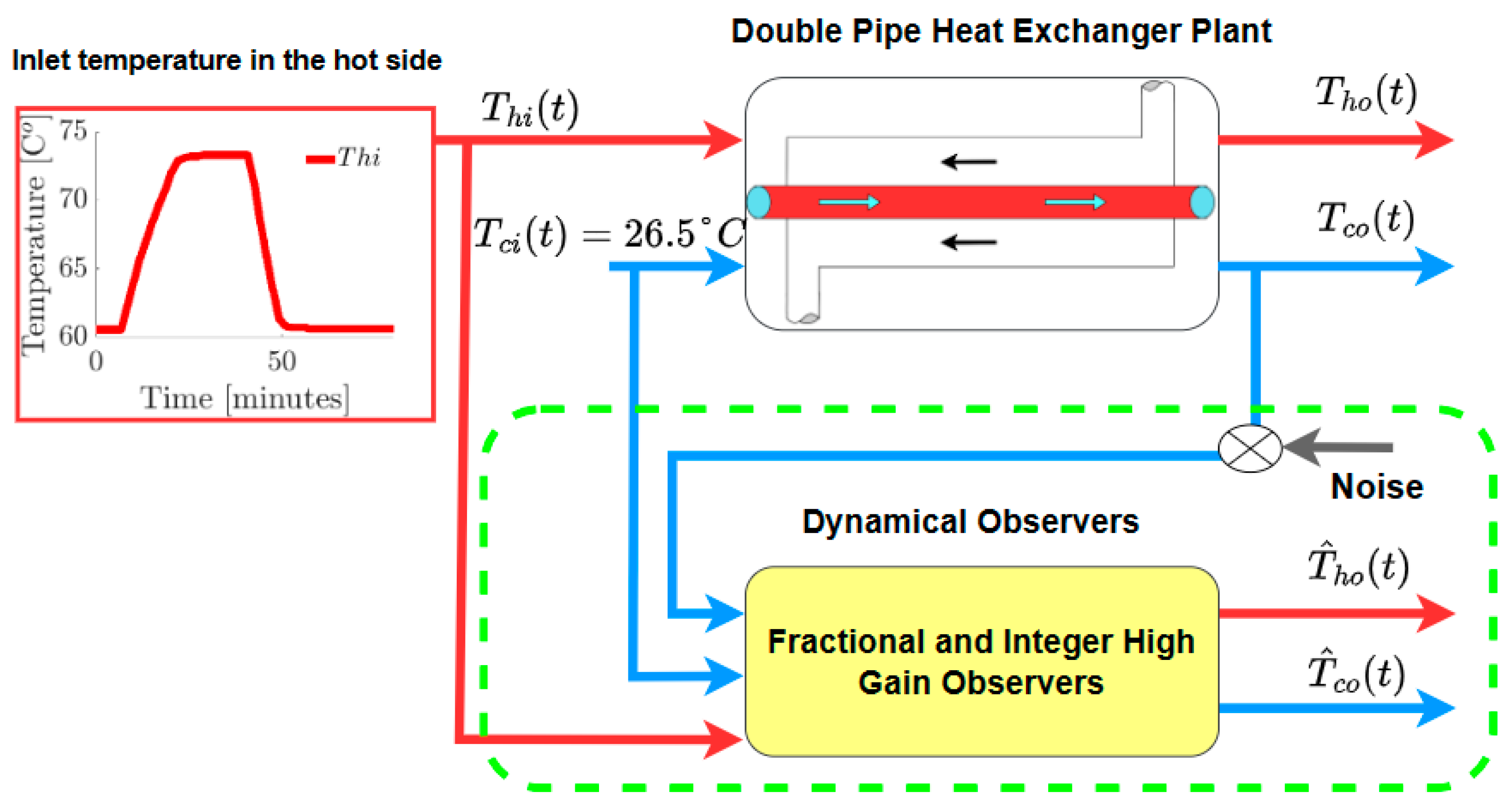
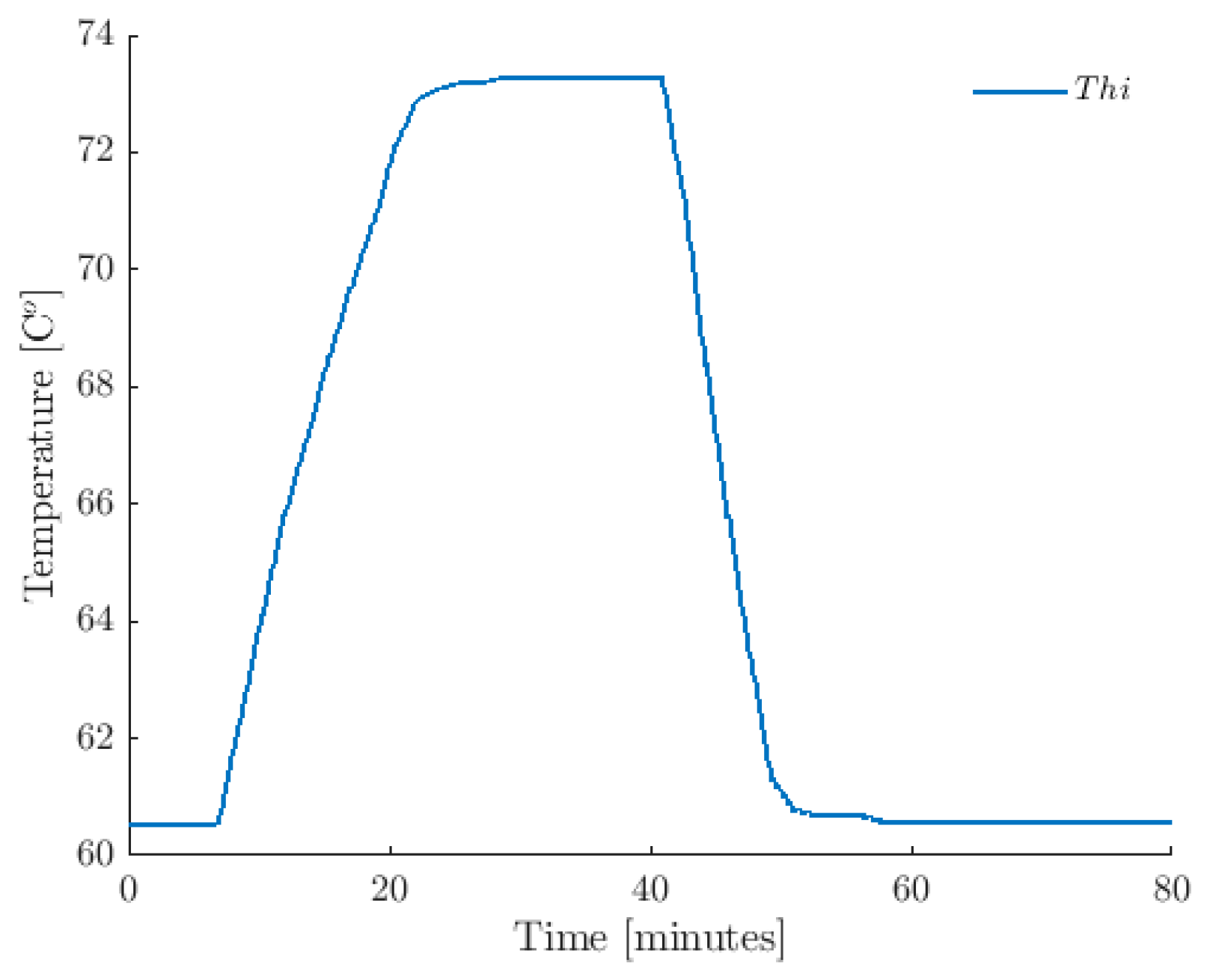
5.1. Experiment Configuration

In order to validate the performance of the proposed FMO-HGO, we set up the experiment shown in Figure 2. For this experiment, we utilized the DPHE pilot plant RCT 100, operating under the conditions specified in Table 2. We selected as inputs to the observers (both integer and fractional HGOs) the inlet temperature data on the hot side shown in Figure 3, the inlet temperature on the cold side, which was fixed to 26.5 °C, and the data measurement of the outlet temperature on the cold side. Additionally, we assumed that the process operates with a constant heat transfer coefficient, U . The experiment involves estimating the outlet temperatures in the cold as well as hot sides using both integer and fractional-order observers from the measurements of the inlet temperatures on the hot side T h i and the outlet temperature on the cold side T c o . The initial conditions of the DPHE were T c o = 36.10 °C and T h o = 55.9 °C. The observer initial conditions were selected to be quite different from the initial conditions of the process, and the observer gains were tuned at θ = 1 . We performed all our tests using a personal computer with 8 GB of RAM and an Intel Core i5 processor of eighth generation. The numerical complexity of the simulation yields on the fact that, since there is a memory trace associated with each derivative, this memory impacts the computational resources because it turns bigger in size when the time increases. The memory trace is the summation part of Equation (34), and the numerical simulation represents a matrix that is growing in each time step, meaning that when time increases, the computational resources start to be limited. Evidently, if we want to implement the FMO-HGO in a different device, such as a microcontroller or microprocessor, we need to take the numerical complexity into account. Fortunately, nowadays, these types of devices have all the computational and memory resources to perform our FMO-HGO without any problem.

5.2. Performance Analyses of the Proposed FMO-HGO

We systematically analyze the performance of the FMO-HGO in different scenarios. First, we conduct a test under ideal conditions, that is, where there is no noise in the measured signal ( T c o ) and no change in the observer gain parameter ( θ ). In the second case, we added noise to the measured signal. Finally, the third case considers a scenario in which the observer gain parameter is compromised; additionally, the noise added to the measured signal remains the same as in the second case. All our tests were conducted using real data collected from a DPHE process in which non-ideal circumstances occurred. This allows us to prove that the fractional-order dynamics considered in the observer can model real-world processes more accurately than using classical calculus.

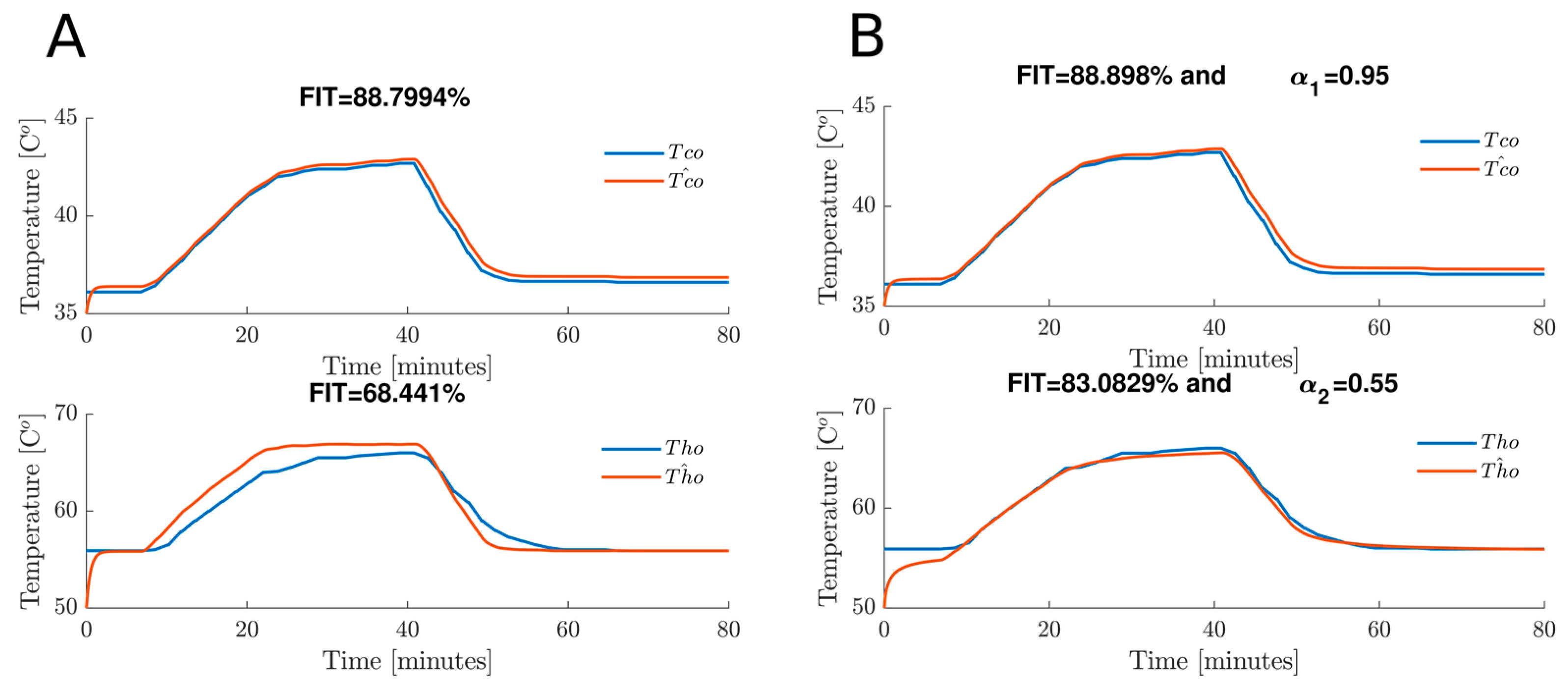
5.2.1. Case 1. Estimation Test under Ideal Conditions

In all our tests, we estimate the outlet temperatures in both the cold as well as hot sides, T c o and T h o , solely by measuring T c o . The data depict the behavior of the outlet temperature on the cold side T c o and the outlet temperature on the hot side T h o ; for different values of inlet temperature on the hot side T h i (the input to the DPHE), all our experiments consider this T h i profile, see Figure 3. We estimate both outlet temperatures, T c o and T h o , using the FMO-HGO designed in this paper, and for comparative purposes, we also use the non-fractional HGO. We show that the FMO-HGO has a better performance than the non-fractional HGO in this case. To quantitatively prove that the performance is better in the fractional-order observer than in the integer (classical) order observer, we use the integral square error (ISE) and integral absolute error (IAE) indices, defined as
  ISE = 0 T 0 e 2 ( t ) d t ,   IAE = 0 T 0 | e ( t ) | d t .
We decided to use the ISE and IAE indices in order to determinate the robustness of the FMO-HGO and the HGO. The ISE and IAE indices provide a quantitative analysis of the performance in both observers (classical and fractional), that is, a lower value in both indices means a better and robust signal estimation.
Also, to measure how much better the FMO-HGO is at reproducing output measurements, the normalized root-mean-square error (NRMSE) criterion is used, which provides a percentage value representing the fit. This criterion is defined as
  FIT = D m ( : , i ) D e ( : , i ) D m ( : , i ) m e a n ( D m ( : , i ) ) ,
where D m represents the data measurements of the process, D e represents the data estimated for the observer, and i represents the number of samples. The use of the FIT criterion allows us to determinate the accuracy of the estimated signals, which means that the larger the value of FIT, the more accurate the measured signal is.
In Figure 4A, we present the estimation of T h o and T c o using the integer order HGO; we can see the system’s behavior (real data) and the observer’s estimation. In Figure 4B, the same scenario is depicted, but this time using the fractional-order HGO; note that the FMO-HGO can estimate more accurately both states, T c o and T h o , than the integer order HGO. As shown in Figure 4B, the fractional orders employed were α 1 = 0.95 and α 2 = 0.55 for T c o and T h o , respectively. This case does not involve the addition of noise or any change in the observer parameters. Moreover, in Figure 4A, we can see that the FIT for T c o and T h o is 88.79% and 68.44%, respectively; in contrast, in Figure 4B, the FIT for T c o and T h o is 88.89% and 83.08%, respectively. Figure 5A–D show that ISE and IAE have a better performance in the fractional observer than in the classical one. In general, for this case, we can conclude that the FMO-HGO has a better performance that the classical HGO. In the coming tests, we evaluate both observers under real-world conditions, that is, considering a noise which is added to the measured output and a parameter change in both observers; these conditions will allow us to show that the FMO-HGO is more robust than the classical HGO.

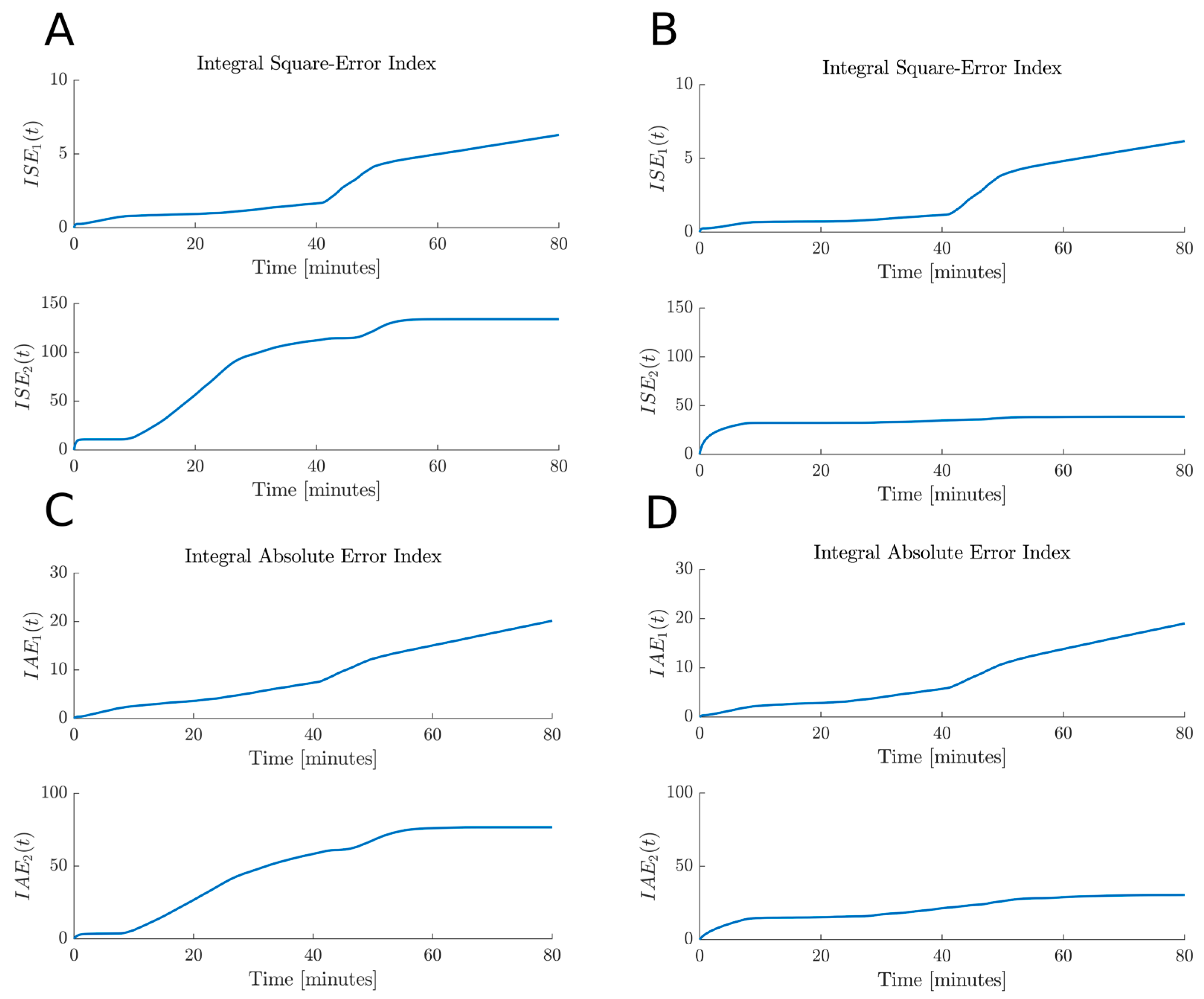
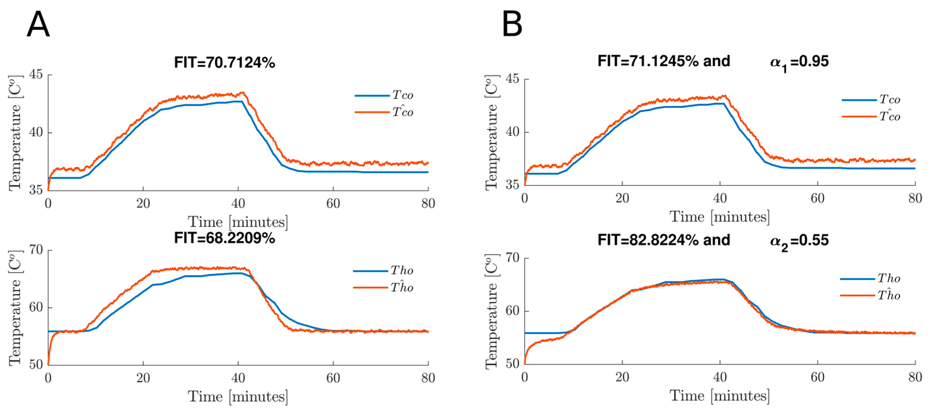
5.2.2. Case 2. Estimation Test under Noise Conditions in the Measurable Variable

This test consisted of the estimation of T c o and T h o as in Case 1, but now in this scenario, the measured signal has a gaussian noise which affects the signals reconstruction of the observer for both outputs. Our results show that by using the FMO-HGO, we can reconstruct both signals more accurately than in the classical HGO, where the reconstruction under this scenario is not warranted. In Figure 6A, we show the performance of the classical observer; note that for T c o and T h o   , the FIT is 88.79% and 68.44%, respectively. On the other hand, the FMO-HGO performance shown in Figure 6B proves that by using different values in each order of the observer, we can recover both signals better than the classical HGO case. The FIT for both signals is above 83%; specifically, for T c o it is 88.79%, and for T h o it is 88.89%. It is evident that by using multi-order in the observer, we can recover both signals better than the classical case. Moreover, our analysis proves that the ISE and IAE show a better performance for the fractional-order observer than for the classical order observer since the values for both indices are lower in the fractional case than in the classical case (see Figure 7A–D).

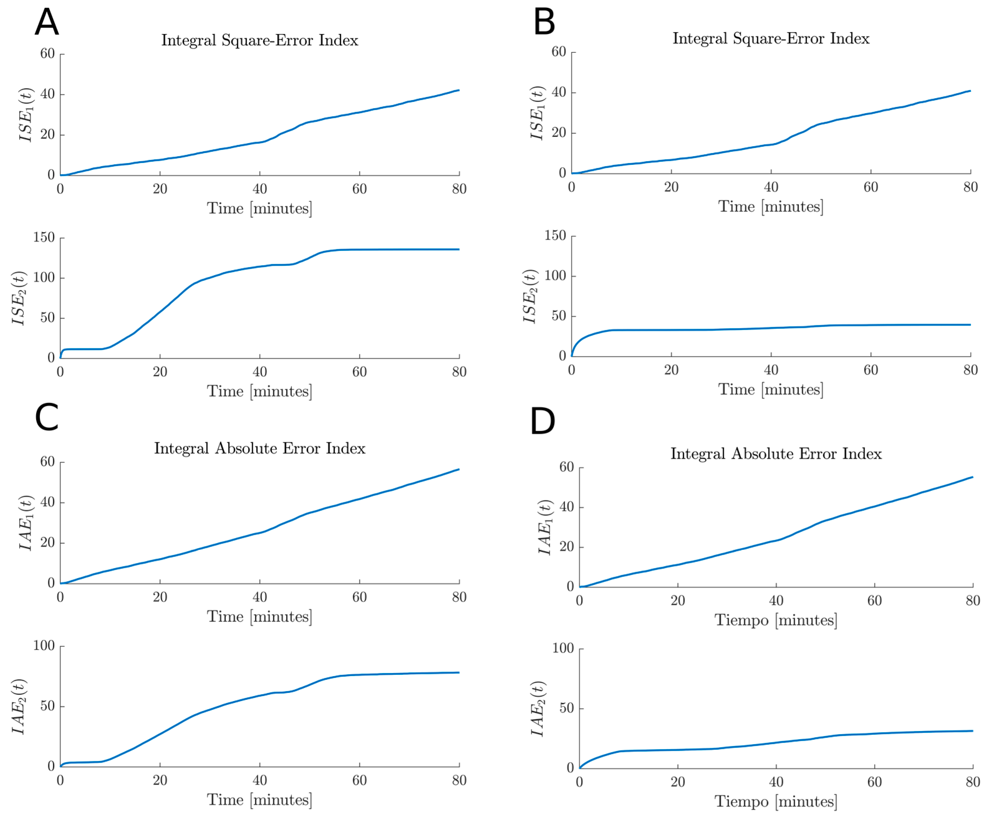
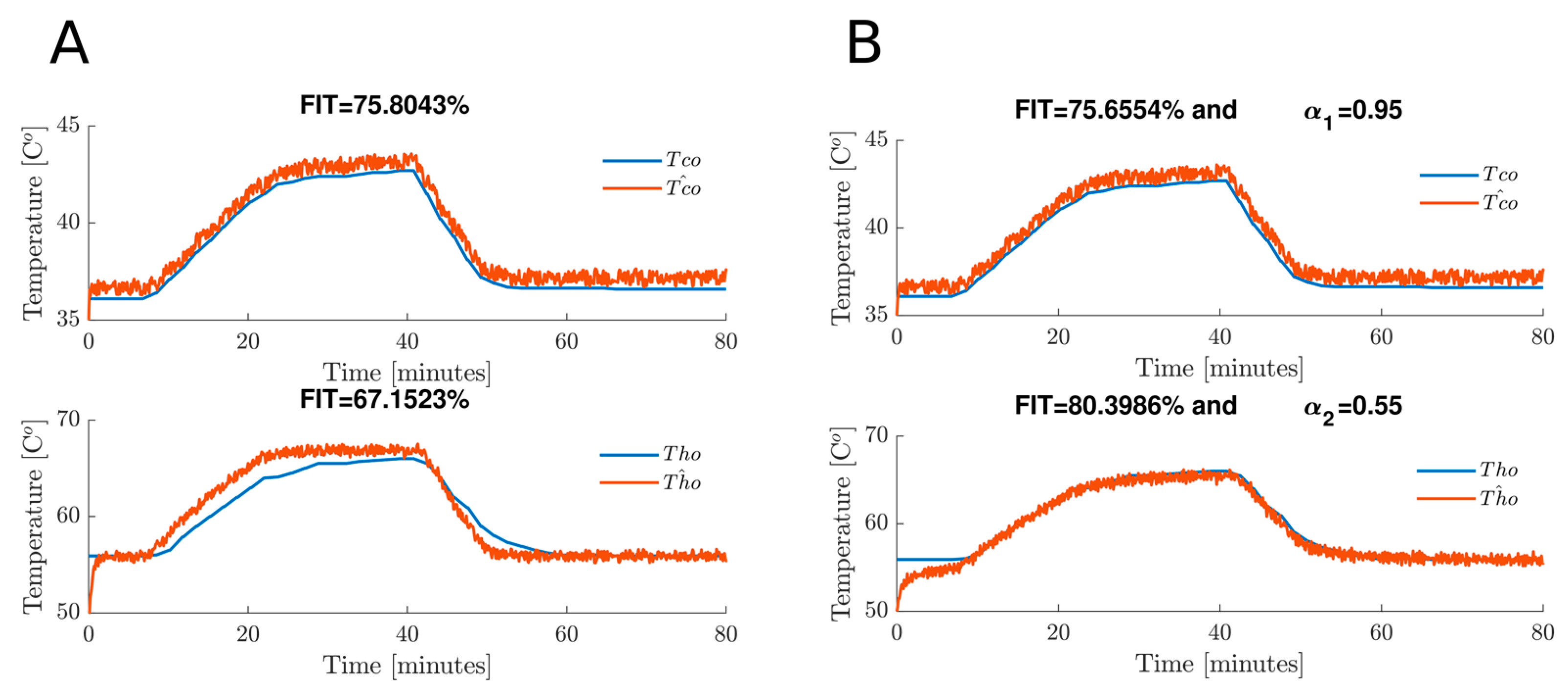
5.2.3. Case 3. Estimation Test Involving Noise Conditions in the Measurable Variable and a Change in the Observer Gains

Finally, in this case we evaluate the performance of both the integer and fractional-order HGOs, considering that the data measurement of the outlet temperature T c o is contaminated with noise and the gain of the observers was selected with a high value at θ = 4. One reason to increase the gain of the observers is that the rate of convergence is directly influenced by the gain of the observer. However, one drawback of this practice is that the observer becomes more susceptible to noise. Therefore, with this test we demonstrate that the FMO-HGO has better robustness properties to noise than the classical (integer order) HGO when a change in the observer parameter occurs.
Figure 8 shows a comparison between the estimated outlet temperatures against the experimental data outlet temperatures. Figure 8A corresponds to the estimated outlet temperature using the integer order HGO, while Figure 8B corresponds to the estimated outlet temperature using the FMO-HGO. The results of the estimated outlet temperature on the hot side show that both integer and fractional HGOs predict values close to the experiment data T h o , with an FIT of 70.8043% and 70.6554%, respectively. These results indicated that there is no difference in the performance estimation of the outlet temperature on the hot side when using both integer and fractional-order HGOs. However, the outstanding finding of the results is that the estimated outlet temperature on the cold side for the FMO-HGO predicts values closer to the experiment data T c o than the integer order HGO, with an FIT of 80.3936% and 67.1523%, respectively. Therefore, the FIT of the proposed FMO-HGO shown is better than the FIT of the classical (integer order) HGO.
Additionally to the FIT criteria, we use the ISE and IAE indices to show that under both data, noisy conditions and a change in the observer gain, the FMO-HGO presents a better performance. Figure 9A,B show the ISE index behavior for the integer and FMO-HGOs. No significant difference in the performance of the estimation of the outlet temperature T h o with both observers is observed. However, the improvement in the estimate of the outlet temperature T c o with the FMO-HGO is evident. A similar situation with the IAE index is shown in Figure 9C,D. Overall, these results provide a better understanding on how accurately and robust the FMO-HGO is against the HGO; although no significant difference occurred in the estimation of T h o , this was due to the outstanding results of T c o , where the ISE and IAE indices are much lower. Previous results allow us to conclude that the FMO-HGO is more accurate and robust than the HGO.
In summary, we present in Table 3 a comparison between the classical HGO and the FMP-HGO performance under the three scenarios. In Case 1, both observers have a good estimation for T c o ; however, the FMO-HGO provides a better estimation of T h o ; this accuracy is evident when we computed the FIT, which is above 83%. The ISE and IAE indices’ final values are lower for the FMO-HGO than for the HGO for both estimated temperatures. We obtained a similar result for Case 2: the FIT computed for the FMO-HGO is better than the FIT in the HGO on both temperatures, but it outstands in T h o ; in addition, the ISE and IAE final values are lower in the fractional case than in the classical case. This test allows us to determinate that the FMO-HGO is more robust than the classical HGO under noise circumstances. Finally, Case 3 has a similar FIT in T c o temperature, but this is better in T h o , where the FIT is above 80%; the ISE and IAE indices show a better performance in the fractional case than in the classical case. Previous results demonstrate that the FMO-HGO is more robust than the classical HGO under noise perturbation and parameter change circumstances. We want to emphasize that we tested both observers under the same circumstances in all cases.

6. Conclusions and Discussions

In this paper, we designed a novel fractional multi-order high-gain observer (FMO-HGO) to estimate outlet temperatures in a DPHE process. We systematically validated the performance of the proposed FMO-HGO; we performed several comparisons between the experimental data and the estimated outlet temperatures using both the FMO-HGO and the classical HGO. The results showed that under ideal conditions (without noisy data and a conservative value in the observer gain), both the FMO-GHO and classical HGO exhibit a similar performance. However, when a gaussian noise of 10% was added to the outlet temperature on the cold side T c o , the performance of the proposed FMO-HGO was shown to be better. We concluded that fractional derivative allows us to mitigate the noise effects in the measured signal, which implies that fractional derivative plays a noise filtering role. Additionally, when the observer gain was set up to a high value, the better performance of the FMO-HGO was more evident. The FIT criterion, as well as both the ISE and IAE indices, were used to demonstrate the better performance of the FMO-HGO.
It is notable that the FMO-HGO provides a better performance due to its intrinsic memory associated with the fractional derivative. It has been demonstrated that this characteristic allows us to predict future system behavior and, hence, the system is more robust to change in terms of parameters and noise [30]. As we expected, fractional-order calculus (FOC) provides robustness to the HGO, which in real conditions can guarantee a better estimation than using the non-fractional (classical) HGO. In addition, since we are using the new concept of introducing fractional multi-order in each system equation, this allowed us to expand the degrees of freedom in the system, and we can adjust each equation according to its dynamics. In summary, our work opens a new approach in signal analysis and estimation, which may contribute to a deeper understanding of real complex data of an exchange heat process. For future works, we suspect that this approach can be expanded to other systems with non-Markov behavior in applications such as signal processing, fractional-order synchronization, fractional-order control design, and fault and diagnose estimation. We believe that our approach (fractional-order) can provide a better performance than the classical approach (non-fractional) to such disciplines since we have proved that fractional-order calculus can model non-local phenomena due the intrinsic memory associated with the fractional derivative kernel and its natural property of noise filtering. Finally, we are interested in the study of using different fractional-order calculus definitions in these disciplines.

Author Contributions

Conceptualization, V.B.-J. and A.C.-E.; methodology, V.B.-J. and A.C.-E.; software, A.C.-E. and A.C.-R.; validation, V.B.-J., A.C.-E., M.A.-M., A.C.-R., A.G.-V. and J.G.-M.; formal analysis, V.B.-J., A.C.-E., M.A.-M., A.C.-R., A.G.-V. and J.G.-M.; investigation, V.B.-J., A.C.-E. and J.G.-M.; resources, A.C.-E.; data curation, V.B.-J., M.A.-M. and J.G.-M.; writing—original draft preparation, V.B.-J. and A.C.-E.; writing, A.C.-E. and V.B.-J., review and editing, V.B.-J., A.C.-E., M.A.-M., A.C.-R., A.G.-V. and J.G.-M.; visualization, V.B.-J. and A.C.-E.; supervision, A.C.-E.; project administration, V.B.-J., A.C.-E., M.A.-M. and J.G.-M.; funding acquisition, A.C.-E. All authors have read and agreed to the published version of the manuscript.

Funding

This research received no external funding.

Data Availability Statement

Research data are available upon request to the corresponding author at [email protected].

Acknowledgments

We would like to thank the Mexican people that supported this research through the CONAHCyT (Consejo Nacional de Humanidades, Ciencias y Tecnologías-National Council of Humanities, Sciences and Technologies), México.

Conflicts of Interest

The authors declare no conflict of interest.

References

  1. Alam, T.; Kim, M.-H. A comprehensive review on single phase heat transfer enhancement techniques in heat exchanger applications. Renew. Sustain. Energy Rev. 2018, 81, 813–839. [Google Scholar] [CrossRef]
  2. Omidi, M.; Farhadi, M.; Jafari, M. A comprehensive review on double pipe heat exchangers. Appl. Therm. Eng. 2017, 110, 1075–1090. [Google Scholar] [CrossRef]
  3. Srimuang, W.; Amatachaya, P. A review of the applications of heat pipe heat exchangers for heat recovery. Renew. Sustain. Energy Rev. 2012, 16, 4303–4315. [Google Scholar] [CrossRef]
  4. Li, H.; Wang, Y.; Han, Y.; Li, W.; Yang, L.; Guo, J.; Liu, Y.; Zhang, J.; Zhang, M.; Jiang, F. A comprehensive review of heat transfer enhancement and flow characteristics in the concentric pipe heat exchanger. Powder Technol. 2022, 397, 117037. [Google Scholar] [CrossRef]
  5. Wallhäußer, E.; Hussein, M.; Becker, T. Detection methods of fouling in heat exchangers in the food industry. Food Control 2012, 27, 1–10. [Google Scholar] [CrossRef]
  6. Padhee, S. Controller Design for Temperature Control of Heat Exchanger System: Simulation Studies. WSEAS Trans. Syst. Control 2014, 9, 485–491. [Google Scholar]
  7. Borja-Jaimes, V.; Adam-Medina, M.; López-Zapata, B.Y.; Valdés, L.G.V.; Pachecano, L.C.; Coronado, E.M.S. Sliding Mode Observer-Based Fault Detection and Isolation Approach for a Wind Turbine Benchmark. Processes 2021, 10, 54. [Google Scholar] [CrossRef]
  8. Borja-Jaimes, V.; Adam-Medina, M.; García-Morales, J.; Guerrero-Ramírez, G.V.; López-Zapata, B.Y.; Coronado, E.M.S. Actuator FDI Scheme for a Wind Turbine Benchmark Using Sliding Mode Observers. Processes 2023, 11, 1690. [Google Scholar] [CrossRef]
  9. Diaz-Bejarano, E.; Coletti, F.; Macchietto, S. A Model-Based Method for Visualization, Monitoring, and Diagnosis of Fouling in Heat Exchangers. Ind. Eng. Chem. Res. 2020, 59, 4602–4619. [Google Scholar] [CrossRef]
  10. Nagarsheth, S.H.; Bhatt, D.S.; Hirpara, R.H.; Sharma, S.N. Non-linear filter design for a counter-flow heat exchanger: Some investigations. Int. J. Dyn. Control 2021, 9, 922–934. [Google Scholar] [CrossRef]
  11. Thibault, É.; Désilets, F.L.; Poulin, B.; Chioua, M.; Stuart, P. Comparison of signal processing methods considering their optimal parameters using synthetic signals in a heat exchanger network simulation. Comput. Chem. Eng. 2023, 178, 108380. [Google Scholar] [CrossRef]
  12. Kim, W.; Lee, J.-H. Fault detection and diagnostics analysis of air conditioners using virtual sensors. Appl. Therm. Eng. 2021, 191, 116848. [Google Scholar] [CrossRef]
  13. Wang, J.; Sun, J.; Ge, W.; Zhang, F.; Gao, R.X. Virtual Sensing for Online Fault Diagnosis of Heat Exchangers. IEEE Trans. Instrum. Meas. 2022, 71, 9508708. [Google Scholar] [CrossRef]
  14. Ahilan, C.; Dhas, J.E.R.; Somasundaram, K.; Sivakumaran, N. Performance assessment of heat exchanger using intelligent decision making tools. Appl. Soft Comput. 2015, 26, 474–482. [Google Scholar] [CrossRef]
  15. Sridharan, M. Application of fuzzy logic expert system in predicting cold and hot fluid outlet temperature of counter-flow double-pipe heat exchanger. In Advanced Analytic and Control Techniques for Thermal Systems with Heat Exchangers; Academic Press: Cambridge, MA, USA, 2020; pp. 307–323. [Google Scholar] [CrossRef]
  16. Apio, A.; Martinelli, G.B.; Trierweiler, L.F.; Farenzena, M.; Trierweiler, J.O. Fouling monitoring of a heat exchanger network of an actual crude oil distillation unit by constrained extended Kalman filter with smoothing. Chem. Eng. Commun. 2023, 210, 2229–2248. [Google Scholar] [CrossRef]
  17. Kazaku, J.K.; Dochain, D.; Winkin, J.; Kahilu, M.M.; Kasongo, J.K.K. Port-Hamiltonian Sliding Mode Observer Design for a Counter-current Heat Exchanger. IFAC-PapersOnLine 2020, 53, 4910–4915. [Google Scholar] [CrossRef]
  18. Han, X.; Li, Z.; Cabassud, M.; Dahhou, B. A comparison study of nonlinear state ob-server design: Application to an intensified heat-exchanger/reactor. In Proceedings of the 2020 28th Mediterranean Conference on Control and Automation, MED 2020, Saint-Raphaël, France, 15–18 September 2020; pp. 162–167. [Google Scholar] [CrossRef]
  19. Khalil, H.K. High-gain observers in nonlinear feedback control. In Proceedings of the 2008 International Conference on Control, Automation and Systems, Seoul, Republic of Korea, 14–17 October 2008. [Google Scholar] [CrossRef]
  20. Ahrens, J.H.; Khalil, H.K. High-gain observers in the presence of measurement noise: A switched-gain approach. Automatica 2009, 45, 936–943. [Google Scholar] [CrossRef]
  21. Monje, C.A.; Chen, Y.; Vinagre, B.M.; Xue, D.; Feliu-Batlle, V. Fractional-Order Systems and Controls: Fundamentals and Applications; Springer Science & Business Media: Berlin, Germany, 2010; Available online: https://books.google.es/books?hl=es&lr=&id=c4fV9WeCiEwC&oi=fnd&pg=PR9&dq=fractional+order+calculus+fundamentals+&ots=E1uXM6iMMF&sig=i7vpaCR8Pin5f2LGSeG-P9-lv9w#v=onepage&q=fractional%20order%20calculus%20fundamentals&f=false (accessed on 1 October 2023).
  22. Gutiérrez, R.E.; Rosário, J.M.; Machado, J.T. Fractional Order Calculus: Basic Concepts and Engineering Applications. Math. Probl. Eng. 2010, 2010, 375858. [Google Scholar] [CrossRef]
  23. Coronel-Escamilla, A.; Tuladhar, R.; Stamova, I.; Santamaria, F. Fractional-order dynamics to study neuronal function. In Fractional-Order Modeling of Dynamic Systems with Applications in Optimization, Signal Processing, and Control; Academic Press: Cambridge, MA, USA, 2022; pp. 429–456. [Google Scholar] [CrossRef]
  24. Tepljakov, A. Fractional-Order Modeling and Control of Dynamic Systems; Springer: Berlin/Heidelberg, Germany, 2017; Available online: https://books.google.es/books?hl=es&lr=&id=NswWDgAAQBAJ&oi=fnd&pg=PP7&dq=fractional+order+calculus&ots=jwao5TX84_&sig=5tF-2ojzCsWNqX1z6_HMjX2a0oM#v=onepage&q=fractional%20order%20calculus&f=false (accessed on 1 October 2023).
  25. Martínez-Fuentes, O.; Martínez-Guerra, R. A high-gain observer with Mittag–Leffler rate of convergence for a class of nonlinear fractional-order systems. Commun. Nonlinear Sci. Numer. Simul. 2019, 79, 104909. [Google Scholar] [CrossRef]
  26. Coronel-Escamilla, A.; Gómez-Aguilar, J.; Torres-Jiménez, J.; Mousa, A.; Elagan, S. Fractional synchronization involving fractional derivatives with nonsingular kernels: Application to chaotic systems. Math. Methods Appl. Sci. 2023, 46, 7987–8003. [Google Scholar] [CrossRef]
  27. Boroujeni, E.A.; Momeni, H.R. Non-fragile nonlinear fractional order observer design for a class of nonlinear fractional order systems. Signal Process. 2012, 92, 2365–2370. [Google Scholar] [CrossRef]
  28. Dinh, T.N.; Kamal, S.; Pandey, R.K. Fractional-Order System: Control Theory and Applications; MDPI AG: Basel, Switzerland, 2023; p. 204. [Google Scholar] [CrossRef]
  29. de Almeida, A.M.; Lenzi, M.K.; Lenzi, E.K. A Survey of Fractional Order Calculus Applications of Multiple-Input, Multiple-Output (MIMO) Process Control. Fractal Fract. 2020, 4, 22. [Google Scholar] [CrossRef]
  30. Coronel-Escamilla, A.; Gomez-Aguilar, J.F.; Stamova, I.; Santamaria, F. Fractional order controllers increase the robustness of closed-loop deep brain stimulation systems. Chaos Solitons Fractals 2020, 140, 110149. [Google Scholar] [CrossRef]
  31. Bettayeb, M.; Djennoune, S.; Al-Saggaf, U.M. High gain observer design for fractional-order non-linear systems with delayed measurements: Application to synchronisation of fractional-order chaotic systems. IET Control Theory Appl. 2017, 11, 3171–3178. [Google Scholar] [CrossRef]
  32. Rodriguez-Mata, A.E.; Bustos-Terrones, Y.; Gonzalez-Huitrón, V.; Lopéz-Peréz, P.A.; Hernández-González, O.; Amabilis-Sosa, L.E. A Fractional High-Gain Nonlinear Observer Design—Application for Rivers Environmental Monitoring Model. Math. Comput. Appl. 2020, 25, 44. [Google Scholar] [CrossRef]
  33. Deng, W.; Li, C.; Guo, Q. Analysis of fractional differential equations with multi-orders. Fractals 2011, 15, 173–182. [Google Scholar] [CrossRef]
  34. Ahmadova, A.; Huseynov, I.T.; Fernandez, A.; Mahmudov, N.I. Trivariate Mittag-Leffler functions used to solve multi-order systems of fractional differential equations. Commun. Nonlinear Sci. Numer. Simul. 2021, 97, 105735. [Google Scholar] [CrossRef]
  35. Diethelm, K.; Ford, N.J. Multi-order fractional differential equations and their numerical solution. Appl. Math. Comput. 2004, 154, 621–640. [Google Scholar] [CrossRef]
  36. Chen, Y.Q.; Petras, I.; Xue, D. Fractional order control—A tutorial. In Proceedings of the 2009 American Control Conference (ACC), St. Louis, MO, USA, 10–12 July 2009; pp. 1397–1411. [Google Scholar]
  37. Yang, Y.; Zhang, H.H. Fractional Calculus with Its Applications in Engineering and Technology; Springer Science and Business Media LLC: Dordrecht, The Netherlands, 2019. [Google Scholar] [CrossRef]
  38. Scherer, R.; Kalla, S.L.; Tang, Y.; Huang, J. The Grünwald–Letnikov method for fractional differential equations. Comput. Math. Appl. 2011, 62, 902–917. [Google Scholar] [CrossRef]
  39. Petráš, I. Fractional-Order Nonlinear Systems; Springer: Berlin/Heidelberg, Germany, 2011; Available online: http://link.springer.com/10.1007/978-3-642-18101-6 (accessed on 4 October 2023).
  40. McGraw-Hill Education. Giorgio Carta, Heat and Mass Transfer for Chemical Engineers: Principles and Applications; McGraw-Hill Education: New York, NY, USA, 2021; Available online: https://www.accessengineeringlibrary.com/content/book/9781264266678 (accessed on 9 July 2023).
  41. Cao, E. Heat Transfer in Process Engineering; McGraw-Hill Education: New York, NY, USA, 2010; Available online: https://www.accessengineeringlibrary.com/content/book/9780071624084 (accessed on 20 September 2023).
  42. Serth, R.W.; Lestina, T.G. Process Heat Transfer: Principles, Applications and Rules of Thumb, 2nd ed.; Elsevier: Amsterdam, The Netherlands, 2014; pp. 1–609. [Google Scholar] [CrossRef]
  43. Bergman, T.L.; Lavine, A.; Incropera, F.P. Fundamentals of Heat and Mass Transfer. 2018. Available online: https://www.wiley.com/en-us/Fundamentals+of+Heat+and+Mass+Transfer%2C+8th+Edition-p-9781119353881 (accessed on 9 July 2023).
  44. Khalil, H.K.; Praly, L. High-gain observers in nonlinear feedback control. Int. J. Robust Nonlinear Control 2014, 24, 993–1015. [Google Scholar] [CrossRef]
  45. Prasov, A.A.; Khalil, H.K. A Nonlinear High-Gain Observer for Systems With Measurement Noise in a Feedback Control Framework. IEEE Trans. Autom. Control 2013, 58, 569–580. [Google Scholar] [CrossRef]
  46. Ball, A.A.; Khalil, H.K. Analysis of a nonlinear high-gain observer in the presence of measurement noise. In Proceedings of the 2011 American Control Conference IEEE, San Francisco, CA, USA, 29 June–1 July 2011; pp. 2584–2589. [Google Scholar] [CrossRef]
  47. Gauthier, J.; Hammouri, H.; Othman, S. A simple observer for nonlinear systems applications to bioreactors. IEEE Trans. Autom. Control 1992, 37, 875–880. [Google Scholar] [CrossRef]
  48. Gauthier, J.; Hammouri, H.; Kupka, I. Observers for nonlinear systems. In Proceedings of the 30th IEEE Conference on Decision and Control, Brighton, UK, 11–13 December 1991; pp. 1483–1489. [Google Scholar] [CrossRef]
  49. Atassi, A.; Khalil, H. Separation results for the stabilization of nonlinear systems using different high-gain observer designs. Syst. Control Lett. 2000, 39, 183–191. [Google Scholar] [CrossRef]
  50. Khalil, H.K. High-Gain Observers in Nonlinear Feedback Control; Society for Industrial & Applied Mathematics (SIAM): Philadelphia, PA, USA, 2017. [Google Scholar] [CrossRef]
Figure 1. Architecture of a double pipe heat exchanger (DPHE).
Axioms 12 01107 g001
Figure 2. DPHE experiment setup to validate the observers (FMO-HGO and HGO).
Axioms 12 01107 g002
Figure 3. Data for the inlet temperature on the hot side of the DPHE.
Axioms 12 01107 g003
Figure 4. Validation of the estimated outlet temperatures using experimental data under ideal conditions. (A) Estimated outlet temperatures using the classical HGO. (B) Estimated outlet temperatures using the proposed FMO-HGO.
Axioms 12 01107 g004
Figure 5. Performance indices of the estimated outlet temperatures using experimental data under ideal conditions. (A) Integral square error using the classical HGO. (B) Integral square error using the FMO-HGO. (C) Integral absolute error using the classical HGO. (D) Integral absolute error using the FMO-HGO.
Axioms 12 01107 g005
Figure 6. Validation of the estimated outlet temperatures using noisy experimental data. (A) Estimated outlet temperatures using the classical HGO. (B) Estimated outlet temperatures using the proposed FMO-HGO.
Axioms 12 01107 g006
Figure 7. Performance indices of the estimated outlet temperatures using noisy experimental data. (A) Integral square error using the classical HGO. (B) Integral square error using the FMO-HGO. (C) Integral absolute error using the classical HGO. (D) Integral absolute error using the FMO-HGO.
Axioms 12 01107 g007
Figure 8. Validation of the estimated outlet temperatures using noisy experimental data and a high observer gain. (A). Estimated outlet temperatures using the classical HGO. (B). Estimated outlet temperatures using the proposed FMO-HGO.
Axioms 12 01107 g008
Figure 9. Performance indices of the estimated outlet temperatures using noisy experimental data and a high observer gain. (A) Integral square error using the classical HGO. (B) Integral square error using the FMO-HGO. (C) Integral absolute error using the classical HGO. (D) Integral absolute error using the FMO-HGO.
Axioms 12 01107 g009
Table 1. Description of the variables and parameters of the DPHE model.
NotationDescriptionNotationDescription
T c i Inlet temperature on the cold side. c p h Specific heat on the hot side.
T h i Inlet temperature on the hot side. ρ c Density of the cold fluid.
T c o Outlet temperature on the cold side. ρ h Density of the hot fluid.
T h o Outlet temperature on the hot side. V c Volume on the cold side.
U Heat transfer coefficient. V h Volume on the hot side.
A c Shell side area. v c Flow rate on the cold side.
A h Tube side area. v h Flow rate on the hot side.
c p c Specific heat on the cold side.--
Table 2. Physical data for the DPHE pilot plant RCT 100.
ParameterValueParameterValue
T c i 26.5 °C c p h 4179 J/(Kg K)
T h i 60.55 °C ρ c 991.8 Kg/m3
T c o 36.10 °C ρ h 983.3 Kg/m3
T h o 55.9 °C V c 1.3499 × 10⁻⁴ m3
U 1050 J/(m2 °C s) V h 1.5512 × 10⁻⁵ m3
A c 0.0154 m2 v c 6.6667 × 10⁻⁶ m3/s
A h 0.0124 m2 v h 1.6667 × 10⁻⁶ m3/s
c p c 4174 J/(Kg °C)--
Table 3. FIT, ISE, and IAE analysis between the experiment data and estimated temperatures with the integer order HGO and the FMO-HGO.
ExperimentNormalized Root-Mean-Square Error FITIntegral Square Error
ISE
Integral Absolute Error
IAE
Case T c o T h o T c o T h o T c o T h o
HGOFMO-HGOHGOFMO-HGOHGOFMO-HGOHGOFMO-HGOHGOFMO-HGOHGOFMO-HGO
1 88.79%88.89%68.44%83.08%6.286.1013438.5120.1619.0176.6530.45
2 70.71%71.12%68.22%82.82%42.2841.04135.839.6756.655.078.2831.48
375.80%75.65%67.15%80.39%28.8428.12144.851.2243.9342.8583.4742.79
Disclaimer/Publisher’s Note: The statements, opinions and data contained in all publications are solely those of the individual author(s) and contributor(s) and not of MDPI and/or the editor(s). MDPI and/or the editor(s) disclaim responsibility for any injury to people or property resulting from any ideas, methods, instructions or products referred to in the content.

