Infinite Horizon Irregular Quadratic BSDE and Applications to Quadratic PDE and Epidemic Models with Singular Coefficients

Abstract

In an infinite time horizon, we focused on examining the well-posedness of problems for a particular category of Backward Stochastic Differential Equations having quadratic growth (QBSDEs) with terminal conditions that are merely square integrable and generators that are measurable. Our approach employs a Zvonkin-type transformation in conjunction with the Itô–Krylov’s formula. We applied our findings to derive probabilistic representation of a particular set of Partial Differential Equations par have quadratic growth in the gradient (QPDEs) characterized by coefficients that are measurable and almost surely continuous. Additionally, we explored a stochastic control optimization problem related to an epidemic model, interpreting it as an infinite time horizon QBSDE with a measurable and integrable drifts.

1. Motivation and Introduction

The study of Backward Stochastic Differential Equations (BSDEs) began in the linear case with Bismut’s work [1], where stochastic integrals were applied in controlling linear quadratic systems. Pardoux and Peng [2] extended this to the nonlinear case, establishing the existence and uniqueness of solutions in multidimensional settings with finite terminal times, a square-integrable terminal condition, and Lipschitz continuous generators. This seminal work stimulated extensive research, leading to various extensions and generalizations.

In the case of an infinite time horizon, Pardoux [3], Pardoux and Zhang [4], and Darling and Pardoux [5] considered BSDEs under conditions where the terminal value $\xi$ is either 0 or $\mathbb{E}\left[e^{\rho T}\right|\xi {|}^2]$ for a constant $\rho >0$ and a random terminal time T. Peng [6] established existence and uniqueness under certain monotonic conditions, albeit with solutions in the spaces of square-integrable adapted processes. Chen [7] proved the existence and uniqueness of BSDEs, when the time horizon T is a stopping time taking values in $[0,\infty ]$, under a specific Lipschitz condition. Based on these results, Chen and Wang [8] studied BSDEs with an infinite terminal time, obtaining solutions in spaces of square-integrable adapted processes for the terminal condition was square-integrable. The drift coefficient was required to verify the Lipschitz condition, with coefficients that are deterministic yet time-dependent, considered to be integrable in $L^1(0,\infty )$ and $L^2(0,\infty )$. Their approach used a fixed-point argument and have provided applications in the pricing of contingent claims in incomplete markets and in economics.

In the framework of Brownian motion, solutions to BSDEs with an ${\mathcal{F}}_T$-measurable terminal condition $\xi$ and a smooth coefficients g are represented by processes ${(Y_t,Z_t)}_{\in [0,T]}$, satisfying the equation:

$$Y_t=\xi +{\int }_t^{T}g(s,Y_s,Z_s)ds-{\int }_t^T{Z}_{s}d{W}_s,0\le t\le T,$$

here $W_{·}$ represents a standard d-dimensional Brownian motion. Initially introduced by Pardoux and Peng [2], these equations have found applications in control theory and PDEs. Pardoux and Peng demonstrated the existence and uniqueness of solutions under smooth square integrability assumptions on $\xi$ and the coefficient $g(t,\omega ,y,z)$ which satisfy Lipschitz condition $(y,z)$ uniformly in $(t,\omega )$. Subsequently, various researchers have relaxed these assumptions, leading to significant advancements in the field.

BSDEs exhibiting quadratic growth in the z-variable have attracted significant interest in fields like PDEs, control theory, finance, and insurance. Significant contributions have been made by researchers such as Bismut [1], Rouge and El Karoui [9], El Karoui et al. [10], and Ankirchner et al. [11]. For example, Briand and Confortola [12] investigated a category of QBSDEs with random time horizon and elliptic PDEs in infinite dimensions. They established the existence and uniqueness of mild solutions for elliptic PDEs with quadratic growth in the solution’s gradient in Hilbert space. This mild solution proved invaluable in applications related to the optimal control of infinite-dimensional nonlinear stochastic systems, particularly in minimizing certain cost functionals over an infinite horizon.

In finance, QBSDEs have found application in solving utility maximization problems, especially in the context of small traders operating within incomplete financial markets. Researchers such as Rouge and El Karoui [9] and Ankirchner et al. [11] have explored utility maximization challenges using diverse techniques, including systems of forward–backward Stochastic Differential Equations (SDEs). Notably, Ankirchner et al. [11] employed QBSDEs in their methodology, specifically relying on the existence result established by Kobylanski [13]. In their approach, determining the optimal trading strategy involved solving a maximization problem. The value function of this optimization problem was intricately connected to the solution of a BSDE, underscoring the significant link between QBSDEs and the pricing and hedging of financial instruments, see [14].

The study of QBSDEs commenced with pioneering works by Kobylanski [13] and Dermoune et al. [15], where two distinct methods yielded the existence of solutions independently. Subsequent extensions of these results have been made by several researchers [16,17,18,19,20]. As an example, Briand and Hu [17] demonstrated the existence of solutions to QBSDEs whenever the value of the BSDE at time T has finite exponential moments. Barrieu and El Karoui [16] provided a monotone stability result for quadratic semi-martingales, thereby existence results of solutions of QBSDEs but still under the exponential moments integrability of the terminal value. Additionally, recent contributions by Bahlali and Hassani [21,22] have proved existence or uniqueness of solutions for a broad a family of QBSDEs having merely continuous coefficients and square-integrable final conditions. Their innovative approach, based in Itô–Krylov’s formula and a Zvonkin-type transformation [23], has pushed the boundaries of QBSDE theory.

In the context of an infinite time horizon, BSDEs have gained substantial traction due to their diverse applications in finance, insurance, stochastic control, and economics. These equations are instrumental in pricing various financial derivatives, such as American options and perpetual options, which lack fixed expiration dates [24,25,26].

Moreover, PDEs of the quadratic type possess unique properties and find applications in numerous scientific and engineering domains. These equations often emerge in mathematical analysis due to their intriguing mathematical properties and contribute to a deeper understanding of PDE theory and techniques. Additionally, QPDEs are prevalent in physical processes, describing phenomena such as heat propagation and wave dynamics. They are closely linked to nonlinear dynamics and can portray complex behaviors in physical systems, including solution formation and wave interactions. In finance, QPDEs play a fundamental role in option pricing and risk management. A classic example is the well-known Black–Scholes equation [27,28]. Variants of these equations, specifically those linked to options pricing and characterized by quadratic growth in the gradient, have been explored in previous works such as [29]. By imposing specific monotonicity conditions, the well posedness within an extensive space for forward–backward stochastic differential equations in an infinite time horizon setting has been established in [30]. Subsequently, they provided probabilistic interpretations for a wide range of quasi-linear elliptic PDEs in a comprehensive spatial context via the solutions derived from FBSDEs in an infinite time horizon.

In this paper, our research has two primary objectives. The first motivation is to establish a probabilistic representation for PDEs of a quadratic form, expressed as:

$$\begin{array}{c}\hfill \left\{\begin{array}{ccc}\hfill \left({\partial }_{t}v+\mathcal{L}v\right)(t,x)+f\left(v\right){\left|\sigma v_x\right|}^2(t,x)& =& 0\mathrm{on}[0,+\infty )\times \mathbb{R},\hfill \\ \\ \hfill v(\infty ,x)& =& \psi \left(x\right),x\in \mathbb{R},\hfill \end{array}\right.\end{array}$$

where the function f is considered to be a measurable and integrable function. Additionally, $\mathcal{L}$ represents a second-order differential operator, which will be explicitly defined below in (8).

The second objective of our study involves finding a probabilistic representation for the optimal control of a specific objective functional J associated with an epidemic model that may have irregular inputs or control, of which the details are reported in Section 4.

Both of these problems can be interpreted in the context of infinite time horizon BSDE.

The primary focus of this paper is twofold:

Firstly, in Section 2, we investigate the well-posedness of solutions for a specific class of QBSDEs. The terminal condition $\xi$ is assumed to be square-integrable, and the generator g is taken as ${\eta }_{·}+f\left(y\right){\left|z\right|}^2$. Here, the function f is assumed to be integrable over the entire space $\mathbb{R}$.

Secondly, in Section 3, we establish probabilistic representations for certain QPDEs with a terminal condition within the framework of Markovian QBSDEs.

The subsequent sections are organized as follows: Section 2 provides definitions, notations, and the main result. In Section 3, we demonstrate the existence of viscosity solutions for a particular class of QPDEs associated with our Markovian BSDEs featuring quadratic coefficients. Section 4 illustrates an application of infinite time horizon QBSDEs to a controlled epidemic model with vaccination.

2. Main Result

2.1. Notations

Consider a standard d-dimensional Brownian motion ${\left(W_t\right)}_{t\ge 0}$ defined on a complete filtered probability space ${(\Omega ,\mathcal{F},{\mathcal{F}}_t)}_{t\ge 0},\mathbb{P})$. ${\left({\mathcal{F}}_t\right)}_{t\ge 0}$ stands for the natural filtration generated by $W_{·}$, where ${\mathcal{F}}_0$ contains all $\mathbb{P}$-null sets of $\mathcal{F}$ and ${\mathcal{F}}_{\infty }={\vee }_{t\ge 0}{\mathcal{F}}_t$. For notational simplicity, the Euclidean norm of an element $x\in {\mathbb{R}}^n$ will be denoted by $\left|x\right|$. We shall use the symbol ∞ for $+\infty$ and write Y instead of ${\left(Y_t\right)}_{t\ge 0}$.

Let us introduce the following spaces:

• ${\mathcal{M}}^2$ is the space of ${\left({\mathcal{F}}_t\right)}_{t\ge 0}$-adapted processes Z in ${\mathbb{R}}^d$ such that

  $${\int }_0^{\infty }\mathbb{E}{\left|Z_s\right|}^{2}ds<\infty .$$
• ${\mathcal{L}}^2$ is the space of ${\left({\mathcal{F}}_t\right)}_{t\ge 0}$-adapted processes Z in ${\mathbb{R}}^d$ satisfying

  $${\int }_0^{\infty }{\left|Z_s\right|}^{2}ds<\infty \mathbb{P}-\mathrm{a}.\mathrm{s}.$$
• ${\mathcal{S}}^2$ is the set of $\mathbb{R}$-valued, continuous, and ${\left({\mathcal{F}}_t\right)}_{t\ge 0}$-adapted processes Y such that

  $$\mathbb{E}\left[\underset{t\ge 0}{sup}{\left|Y_t\right|}^2\right]<\infty .$$
• ${\mathcal{W}}_{p,loc}^2\left(\mathbb{R}\right)$ represents the Sobolev space consisting of functions u defined on $\mathbb{R}$ for which both u and its generalized derivatives $u^{\prime }$ and $u^{″}$ belong to $L_{loc}^p\left(\mathbb{R}\right)$.
• $L^p(\Omega )$ is the collection of $\mathbb{R}$-valued ${\mathcal{F}}_{\infty }$-measurable random variables $\xi$ with

  $${\mathbb{E}\left|\xi \right|}^p<\infty ,p\ge 1.$$
• $\mathcal{P}$ denotes the $\sigma$-algebra of predictable sets on $[0,\infty )\times \Omega$.

In what follows we are given a random coefficient $g:[0,\infty )\times \Omega \times {\mathbb{R}}^{1+d}\to \mathbb{R}$ which is $\mathcal{P}\otimes \mathcal{B}\left(\mathbb{R}\right)\otimes \mathcal{B}\left({\mathbb{R}}^d\right)$-measurable and satisfies the conditions:

$\left(\mathbf{H}\mathbf{1}\right)$

For all $(y,z)\in {\mathbb{R}}^{1+d},g(·,y,z)$ is a stochastic process that is progressively measurable such that

$${\int }_0^{\infty }\mathbb{E}\left|g(t,0,0)\right|dt<\infty .$$

$\left(\mathbf{H}\mathbf{2}\right)$

There exists two non-random functions $\alpha (·)$ and $\beta (·)$ such that, for all

$(y_i,z_i)\in {\mathbb{R}}^{1+d},i=1,2$, we have, $\mathbb{P}$-a.s.:

$$|g(t,y_1,z_1)-g(t,y_2,z_2)| \le \alpha \left(t\right)|y_1-y_2| + \beta \left(t\right)|z_1-z_2|,t\in [0,\infty ),$$

and

$${\int }_0^{\infty }\left(\alpha \left(t\right)+{\beta }^2\left(t\right)\right)dt<\infty .$$

$\left(\mathbf{H}\mathbf{3}\right)$

$\xi \in L^2(\Omega )$.

The integral form of one-dimensional BSDE with terminal value $\xi$ is formulated as

$$Y_t=\xi +{\int }_t^{\infty }g(s,Y_s,Z_s)ds-{\int }_t^{\infty }{Z}_{s}d{W}_s,t\in [0,\infty ),\left(\mathrm{eq}(\xi ,g)\right).$$

The terms $\xi$ and g stand for the inputs of the BSDE equation, referred to as $\mathrm{eq}(\xi ,g)$.

Definition 1.

A solution to $\mathrm{eq}(\xi ,g)$ is a pair of stochastic processes $(Y,Z)$ belonging the product space ${\mathcal{S}}^2\times {\mathcal{M}}^2$ that satisfies the above integral equation.

It is well known (see, for instance, [7,8]), that under $\left(\mathbf{H}\mathbf{1}\right)$–$\left(\mathbf{H}\mathbf{3}\right)$, equation eq$(\xi ,g)$ admits a unique solution.

A BSDE is referred to as quadratic when its generator exhibits, at most, quadratic growth concerning the z variable.

We will now consider additional assumptions that are required for future analysis:

$\left(\mathbf{H}\mathbf{4}\right)$

There exists a non-negative random coefficient ${\eta }_{·}\in L^1([0,\infty )\times \Omega )$ and a measurable function f such that for every $(t,\omega ,y,z)$:

$$g(t,\omega ,y,z)={\eta }_t+{f\left(y\right)\left|z\right|}^2\mathbb{P}\otimes dt-\mathrm{a}.\mathrm{e}.\mathrm{and}{\int }_{\mathbb{R}}\left|f\left(x\right)\right|dx<\infty .$$

Our main tool for the next will be appropriate application of Itô–Krylov’s formula established in [22]. For this, we recall it in the theorem below.

Theorem 1.

Under assumptions $\left(\mathbf{H}\mathbf{3}\right)$ and $\left(\mathbf{H}\mathbf{4}\right)$ we denote by $(Y,Z)$ a solution in ${\mathcal{S}}^2\times {\mathcal{L}}^2$ of the BSDE eq$(\xi ,g)$. For any deterministic function u within the space ${\mathcal{C}}^1\left(\mathbb{R}\right)\cap {\mathcal{W}}_{1,loc}^2\left(\mathbb{R}\right)$, we have

$$u\left(Y_t\right)=u\left(Y_0\right)+{\int }_0^t{u}^{\prime }\left(Y_s\right)d{Y}_s+\frac{1}{2}{\int }_0^t{u}^{″}\left(Y_s\right){\left|Z_s\right|}^{2}ds.$$

Note that, the authors of [22] have named this result as the Itô–Krylov formula. It is shown in a finite time interval $[0,T]$, but it remains valid when T is infinite.

The following Lemma will be our basic tool in the solvability of eq$(\xi ,{\eta }_{·}+f\left(y\right)|z{|}^2)$. One can refer to [22] for more details.

Lemma 1.

For a given function f belonging to $L^1\left(\mathbb{R}\right)$, we define

$$u\left(x\right):={\int }_0^{x}exp\left(2{\int }_0^{y}f\left(t\right)dt\right)dy,$$

The non-negative function u satisfies the properties listed below,

(i)

$u\in {\mathcal{C}}^1\left(\mathbb{R}\right)\cap {\mathcal{W}}_{1,loc}^2\left(\mathbb{R}\right)$ and for all most every x, $u^{″}\left(x\right)-2f\left(x\right)u^{\prime }\left(x\right)=0$.

(ii)

u is a bijective mapping the whole real line to itself.

(iii)

The inverse function $u^{-1}$ is both continuously differentiable on $\mathbb{R}$ and locally in the Sobolev space ${\mathcal{W}}_{1,loc}^2\left(\mathbb{R}\right)$.

(iv)

For any pair of real numbers x and y, there exist positive constants m and M independent on x and y satisfying the following inequalities

$$m\le |x-y|\le \left|u\right(x)-u(y\left)\right|\le M|x-y|.$$

and

$$m\le |x-y|\le |u^{-1}\left(x\right)-u^{-1}\left(y\right)|\le M|x-y|.$$

(v)

Moreover, if f is continuous, then both u and $u^{-1}$ belong to the class ${\mathcal{C}}^2$.

Proposition 1.

Assuming the fulfillment of condition ($\mathbf{H}\mathbf{3}$), consider a globally integrable function f on $\mathbb{R}$. The BSDE eq$(\xi ,{\eta }_{·}+f\left(y\right)|z{|}^2)$ admits a unique solution $(Y,Z)\in {\mathcal{S}}^2\times {\mathcal{M}}^2$ if and only if the BSDE eq$(u\left(\xi \right),u^{\prime }\left(u^{-1}\left(y\right)\right){\eta }_{·})$ posses a unique solution in ${\mathcal{S}}^2\times {\mathcal{M}}^2$.

Proof. 

Suppose that $(Y,Z)$ is a solution of the BSDE eq$(\xi ,{\eta }_{·}+f\left(y\right)|z{|}^2)$, then consider the function u as defined in Lemma 1. Applying Itô–Krylov’s formula to $u\left(Y_t\right)$ yields:

$$u\left(Y_{\infty }\right)=u\left(Y_t\right)+{\int }_t^{\infty }{u}^{\prime }\left(Y_s\right)d{Y}_s+\frac{1}{2}{\int }_t^{\infty }{u}^{″}\left(Y_s\right){\left|Z_s\right|}^{2}ds.$$

Thanks to Lemma 1 - $\left(i\right)$ and the fact that $u\left(Y_{\infty }\right)=u\left(\xi \right)$, the equation reads

$$\begin{array}{ccc}\hfill u\left(\xi \right)& =& u\left(Y_t\right)-{\int }_t^{\infty }{u}^{\prime }\left(Y_s\right)\left[{\eta }_s+f\left(Y_s\right){\left|Z_s\right|}^2\right]ds\hfill \\ & & +{\int }_t^{\infty }{u}^{\prime }\left(Y_s\right)Z_{s}d{W}_s+\frac{1}{2}{\int }_t^{\infty }2f\left(Y_s\right)u^{\prime }\left(Y_s\right){\left|Z_s\right|}^{2}ds,\hfill \\ & =& u\left(Y_t\right)-{\int }_t^{\infty }{u}^{\prime }\left(Y_s\right){\eta }_{s}ds+{\int }_t^{\infty }{u}^{\prime }\left(Y_s\right)Z_{s}d{W}_s.\hfill \end{array}$$

Define ${\tilde{Y}}_t=u\left(Y_t\right)$ and ${\tilde{Z}}_t=u^{\prime }\left(Y_t\right)Z_t$. Since $(Y,Z)\in {\mathcal{S}}^2\times {\mathcal{M}}^2$, the Lipschitz property of u and the uniform boundedness of $u^{\prime }$ ensure that $(\tilde{Y},\tilde{Z})\in {\mathcal{S}}^2\times {\mathcal{M}}^2$.

Conversely, let $(\tilde{Y},\tilde{Z})$ be a solution of eq$(u\left(\xi \right),u^{\prime }\left(u^{-1}\left(y\right)\right){\eta }_{·})$, since the function $u^{-1}$ belongs to ${\mathcal{C}}^1\left(\mathbb{R}\right)\cap {\mathcal{W}}_{1,loc}^2\left(\mathbb{R}\right)$, again the Itô–Krylov’s formula Theorem 1 applied to $u^{-1}\left({\tilde{Y}}_t\right)$ leads to

$$\begin{array}{ccc}\hfill u^{-1}\left({\tilde{Y}}_{\infty }\right)& =& u^{-1}\left({\tilde{Y}}_t\right)+{\int }_t^{\infty }{\left(u^{-1}\right)}^{\prime }\left({\tilde{Y}}_s\right)d{\tilde{Y}}_s+\frac{1}{2}{\int }_t^{\infty }{\left(u^{-1}\right)}^{″}\left({\tilde{Y}}_s\right){\left|{\tilde{Z}}_s\right|}^{2}ds\hfill \\ & =& u^{-1}\left({\tilde{Y}}_t\right)+{\int }_t^{\infty }{\left(u^{-1}\right)}^{\prime }\left({\tilde{Y}}_s\right){\tilde{Z}}_{s}d{W}_s\hfill \\ & & -{\int }_t^{\infty }{\left(u^{-1}\right)}^{\prime }\left({\tilde{Y}}_s\right)u^{\prime }\left(u^{-1}\left({\tilde{Y}}_s\right)\right){\eta }_{s}ds+\frac{1}{2}{\int }_t^{\infty }{\left(u^{-1}\right)}^{″}\left({\tilde{Y}}_s\right){\left|{\tilde{Z}}_s\right|}^{2}ds.\hfill \end{array}$$

(1)

$${\left(u^{-1}\right)}^{\prime }\left(x\right)=\frac{1}{u^{\prime }\left(u^{-1}\left(x\right)\right)}\mathrm{and}{\left(u^{-1}\right)}^{″}\left(x\right)=-\frac{u^{″}\left(u^{-1}\left(x\right)\right)}{{\left(u^{\prime }\left(u^{-1}\left(x\right)\right)\right)}^3}.$$

(2)

Denote by $Y_s=u^{-1}\left({\tilde{Y}}_t\right)$ and $Z_s={\left(u^{-1}\right)}^{\prime }\left({\tilde{Y}}_s\right){\tilde{Z}}_s$, thus

$${\left(u^{-1}\right)}^{″}\left({\tilde{Y}}_s\right)|{\tilde{Z}}_s{|}^2=-\frac{u^{″}\left(Y_s\right)}{{\left(u^{\prime }\left(Y_s\right)\right)}^3}|{\tilde{Z}}_s{|}^2=-\frac{2f\left(Y_s\right)}{{\left(u^{\prime }\left(Y_s\right)\right)}^2}|Z_s{|}^2{u}^{\prime }{\left(u^{-1}\left({\tilde{Y}}_s\right)\right)}^2=-2f\left(Y_s\right){\left|Z_s\right|}^2,$$

since $u^{″}\left(x\right)=2f\left(x\right)u^{\prime }\left(x\right)$. Consequently, by substituting in (1), we obtain

$$d{\tilde{Y}}_t=-u^{\prime }\left(u^{-1}\left({\tilde{Y}}_t\right)\right){\eta }_{t}dt+u^{\prime }\left(Y_t\right)Z_{t}d{W}_t.$$

Therefore, with the above notations, we obtain

$$Y_t=\xi +{\int }_t^{\infty }\left({\eta }_s+f\left(Y_s\right){\left|Z_s\right|}^2\right)ds-{\int }_t^{\infty }{Z}_{s}d{W}_s.$$

Clearly, $(Y,Z)$ verifies the equation eq$(\xi ,{\eta }_{·}+f\left(y\right)|z{|}^2)$. Observe that $(\tilde{Y},\tilde{Z})\in {\mathcal{S}}^2\times {\mathcal{M}}^2$, then thanks to the property $\left(iv\right)$ of u, we easily show that $(Y,Z)\in {\mathcal{S}}^2\times {\mathcal{M}}^2.$ □

Corollary 1.

Suppose that f is a bounded and globally-integrable on the real line $\mathbb{R}$. Under ($\mathbf{H}\mathbf{3}$) and ($\mathbf{H}\mathbf{4}$), the equation eq$(u\left(\xi \right),u^{\prime }\left(u^{-1}\left(y\right)\right){\eta }_{·})$ possesses a unique solution in ${\mathcal{S}}^2\times {\mathcal{M}}^2$.

Proof. 

Certainly, given that $\xi$ is square integrable, the transformed variable $\tilde{\xi }=u\left(\xi \right)$ also remains square integrable, owing to the Lipschitz continuity of u. Moreover, the stochastic process ${\left(u^{\prime }\left(u^{-1}\left(0\right)\right){\eta }_t\right)}_{t\ge 0}$ satisfies the assumption ($\mathbf{H}\mathbf{4}$), and for each $t\ge 0$, the mapping $y⟼u^{\prime }\left(u^{-1}\left(y\right)\right){\eta }_t$ is Lipschitz continuous thanks to the properties of u and the boundedness of the function f. □

Remark 1.

If ${\eta }_{·}\equiv 0$, then eq$(\xi ,f\left(y\right)|z{|}^2)$ has a unique solution whenever $\xi \in L^2(\Omega ,{\mathcal{F}}_{\infty })$ and $f\in L^1\left(\mathbb{R}\right)$. That is, the boundedness is not required for f in this case.

Remark 2.

For a given adapted process ${\left(X_t\right)}_{t\ge 0}$ and a measurable bounded function $K:[0,\infty )\times {\mathbb{R}}^n\to \mathbb{R}$ such that ${\int }_0^{\infty }\mathbb{E}\left|K\right(s,X_s|ds$ is finite, consider the following QBSDE

$$Y_t=\xi +{\int }_t^{\infty }(K(s,X_s)+f\left(Y_s\right)|Z_s{|}^2)ds-{\int }_t^{\infty }{Z}_{s}d{W}_s.$$

(3)

Concrete motivation for studying this class of BSDE will discussed in Section 4.

Applying phase space transformation as before, we show that $(Y,Z)$ is a solution of (3) if and only if $(\tilde{Y},\tilde{Z})=(u\left(Y_t\right),u^{\prime }\left(Y_s\right)Z_s)$ is a solution of

$${\tilde{Y}}_t=u\left(\xi \right)+{\int }_t^{\infty }{u}^{\prime }\left(u^{-1}\left({\tilde{Y}}_s\right)\right)K(s,X_s)ds-{\int }_t^{\infty }{\tilde{Z}}_{s}d{W}_s.$$

(4)

To prove that the equation (4) admits a solution, it suffices to verify that the new generator

$$g(s,\omega ,y):=u^{\prime }\left(u^{-1}\left(y\right)\right)K(s,X_s),$$

fulfills the assumptions of existence and/or uniqueness for classical BSDEs. Indeed:

1. 

The stochastic process $g(s,\omega ,0)$ is progressively measurable and satisfies the integrability condition

$$\begin{array}{ccc}\hfill {\int }_0^{\infty }\mathbb{E}\left|g(s,·,0)\right|ds& =& {\int }_0^{\infty }|u^{\prime }\left(u^{-1}\left(0\right)\right)\left|\mathbb{E}\right|K(s,X_s)|ds\hfill \\ & \le & M{\int }_0^{\infty }\mathbb{E}\left|K(s,X_s)\right|ds<\infty .\hfill \end{array}$$

2. 

For fixed ω and s, the mapping $y⟼g(s,\omega ,y)=u^{\prime }\left(u^{-1}\left(y\right)\right)K(s,X_s)$ is Lipschitz continuous for a bounded and integrable function f over the whole space $\mathbb{R}$.

Corollary 2.

We consider the following forward–backward system

$$\begin{array}{c}\hfill \left\{\begin{array}{ccc}\hfill d{X}_t^{s,x}& =& b(t,X_t^{s,x})ds+\sigma (t,X_t^{s,x})d{W}_t,s\ge 0,t\in [s,\infty ),\hfill \\ \hfill X_t^{t,x}& =& x\in {\mathbb{R}}^n.\hfill \end{array}\right.\end{array}$$

(5)

and

$$\begin{array}{c}\hfill \left\{\begin{array}{ccc}\hfill -d{Y}_t^{s,x}& =& F(t,X_t^{s,x},Y_t^{s,x},Z_t^{s,x})ds-Z_t^{s,x}d{W}_t,s\ge 0,t\in [s,\infty ),\hfill \\ \hfill Y_{\infty }^{s,x}& =& \psi \left(X_{\infty }^{s,x}\right),\hfill \end{array}\right.\end{array}$$

(6)

where $g(t,x,y,z)$, b, and σ are defined respectively on $[0,\infty )\times {\mathbb{R}}^n\times {\mathbb{R}}^n\times {\mathbb{R}}^n\times {\mathbb{R}}^d$, $[0,\infty )\times {\mathbb{R}}^n$ and takes values in ${\mathbb{R}}^n$, ${\mathbb{R}}^n$ and in the space of the $n\times d$ matrices. It is well known that the PDE associated with the forward–backward system (5)–(6) is given by

$$\begin{array}{c}\hfill \left\{\begin{array}{ccc}\hfill ({\partial }_t+\mathcal{L})\left(v\right)(t,x)+g(·,·,v,{\nabla }_{x}v\sigma )(t,x)& =& 0\mathrm{on}[0,\infty )\times {\mathbb{R}}^n\hfill \\ \hfill v(\infty ,x)& =& \psi \left(x\right),x\in {\mathbb{R}}^n,\hfill \end{array}\right.\end{array}$$

(7)

where $\mathcal{L}$ is the operator defined by

$$\begin{array}{ccc}\hfill \mathcal{L}v& =& \sum _{i=1}^n{b}_i\frac{\partial v}{\partial x_i}+\frac{1}{2}\sum _{i,j=1}^n{a}_{ij}\frac{{\partial }^{2}v}{\partial x_i\partial x_j},\hfill \end{array}$$

(8)

here, a is the symmetric positive matrix defined by $a=\sigma {\sigma }^T$. Note that the results in Section 3 correspond to $K\equiv 0$ and $n=1$.

Probabilistic representations of the solutions of Equation (7) and other relations problems can be found in [5,6,12,30,31].

2.2. Comparison Principle

The subsequent outcome enables us to make comparisons between the solutions of QBSDEs of the form eq$(\xi ,f\left(y\right)|z{|}^2)$ in infinite time horizon. Note that we need only to compare the generators with respect to y variable a.e.

Proposition 2.

Let ${\xi }_f$ and ${\xi }_g$ be ${\mathcal{F}}_{\infty }$-measurable and satisfy assumption $\left(\mathbf{H}\mathbf{3}\right)$. Let f and g be two globally-integrable functions on $\mathbb{R}$. Let $(Y^f,Z^f)$ and $(Y^g,Z^g)$ denote solutions of the respective BSDEs eq$({\xi }_f,f\left(y\right)|z{|}^2)$ and eq$({\xi }_g{,g\left(y\right)\left|z\right|)}^2)$. Under assumptions ${\xi }_f\le {\xi }_g$ a.s. and $f\le g$ a.e. solutions are comparable in the following order:

$$Y_t^f\le Y_t^{g}dt\otimes d\mathbb{P}\mathrm{a}.\mathrm{e}.$$

Proof. 

We adapt the proof of [21] to our setting. By Proposition 1, we deduce that $(Y^f,Z^f)$ and $(Y^g,Z^g)$ belong to ${\mathcal{S}}^2\times {\mathcal{M}}^2.$

Due the presence of two coefficients f and g we will make use of the notation $u_f$ and $u_g$ instead of u. Thus for any $h\in L^1\left(\mathbb{R}\right)$ we set

$$u_h\left(x\right):={\int }_0^{x}exp\left(2{\int }_0^{y}h\left(t\right)dt\right)dy.$$

The idea of the proof of the comparison principle consists in applying Itô–Krylov’s formula to $u_f\left(Y_t^g\right)$. This gives

$$\begin{array}{ccc}\hfill u_f\left(Y_{\infty }^g\right)& =& u_f\left(Y_t^g\right)+{\int }_t^{\infty }{u}_f^{\prime }\left(Y_s^g\right)d{Y}_s^g+\frac{1}{2}{\int }_t^{\infty }{u}_f^{″}\left(Y_s^g\right){\left|Z_s^g\right|}^{2}ds,\hfill \\ & & \hfill \\ & =& u_f\left(Y_t^g\right)+{\int }_t^{\infty }{u}_f^{\prime }\left(Y_s^g\right)\left[-g\left(Y_s^g\right){\left|Z_s^g\right|}^{2}ds+Z_s^{g}d{W}_s\right]\hfill \\ & & \hfill \\ & & +\frac{1}{2}{\int }_t^{\infty }{u}_f^{″}\left(Y_s^g\right){\left|Z_s^g\right|}^{2}ds,\hfill \\ & & \hfill \\ & =& u_f\left(Y_t^g\right)-{\int }_t^{\infty }{u}_f^{\prime }\left(Y_s^g\right)g\left(Y_s^g\right){\left|Z_s^g\right|}^{2}ds+{\int }_t^{\infty }{u}_f^{\prime }\left(Y_s^g\right)Z_s^{g}d{W}_s\hfill \\ & & \hfill \\ & & +\frac{1}{2}{\int }_t^{\infty }{u}_f^{″}\left(Y_s^g\right){\left|Z_s^g\right|}^{2}ds.\hfill \end{array}$$

(9)

Given that $u_f^{\prime }\left(Y_s^g\right)Z_s^g\in {\mathcal{M}}^2$, we can infer that the process $M_t={\int }_0^t{u}_f^{\prime }\left(Y_s^g\right)Z_s^{g}d{W}_s$ constitutes a martingale.

Applying again Lemma 1 -$\left(i\right)$, and the equation $u_f^{″}\left(x\right)-2f\left(x\right)u_f^{\prime }\left(x\right)=0$ satisfied by $u_f$, the Equation (9) becomes

$$\begin{array}{ccc}\hfill u_f\left(Y_{\infty }^g\right)& =& u_f\left(Y_t^g\right)+M_{\infty }-M_t-{\int }_t^{\infty }{u}_f^{\prime }\left(Y_s^g\right)g\left(Y_s^g\right){\left|Z_s^g\right|}^{2}ds\hfill \\ & & \\ & & +{\int }_t^{\infty }{u}_f^{\prime }\left(Y_s^g\right)f\left(Y_s^g\right){\left|Z_s^g\right|}^{2}ds.\hfill \\ & =& u_f\left(Y_t^g\right)+M_{\infty }-M_t-{\int }_t^{\infty }{u}_f^{\prime }\left(Y_s^g\right)\left[g\left(Y_s^g\right)-f\left(Y_s^g\right)\right]{\left|Z_s^g\right|}^{2}ds.\hfill \end{array}$$

Notice that the term ${\int }_t^{\infty }{u}_f^{\prime }\left(Y_s^g\right)[g\left(Y_s^g\right)-f\left(Y_s^g\right)]{\left|Z_s^g\right|}^{2}ds$ is positive. Indeed, $u_f^{\prime }\ge 0$ and $f\le g$ a.e. So, we deduce that

$$u_f\left(Y_t^g\right)\ge u_f\left(Y_{\infty }^g\right)-(M_{\infty }-M_t).$$

Since $Y^f$ and $Y^g$ are ${\left({\mathcal{F}}_t\right)}_{t\ge 0}$-adapted processes and $M_{·}$ is a closable martingale, passing to the conditional expectation, we obtain

$$u_f\left(Y_t^g\right)\ge \mathbb{E}\left[u_f\left(Y_{\infty }^g\right|{\mathcal{F}}_t)\right]=\mathbb{E}\left[u_f\left({\xi }_g\right)\left|{\mathcal{F}}_t\right)\right].$$

Remembering that $u_f$ is an increasing function and ${\xi }_g\ge {\xi }_f$, thus

$$u_f\left(Y_t^g\right)\ge \mathbb{E}\left[u_f\left({\xi }_f\right)\left|{\mathcal{F}}_t\right)\right]=u_f\left(Y_t^f\right).$$

Therefore,

$$u_f\left(Y_t^g\right)\ge u_f\left(Y_t^f\right).$$

Now, taking $u_f^{-1}$ in the both sides, we obtain $Y_t^g\ge Y_t^f$, for all $t\in [0,\infty )$, $\mathbb{P}$-a.s. □

The following result is a consequence of the previous one and it will be used in the PDE part.

Corollary 3.

Let ξ satisfy $\left(\mathbf{H}\mathbf{3}\right)$ and assume that $f,g$ lie in $L^1\left(\mathbb{R}\right)$. Denote by $(Y^f,Z^f)$ and $(Y^g,Z^g)$ respective solutions of eq$(\xi ,f\left(y\right)|z{|}^2)$ and eq${(\xi ,g\left(y\right)|z\left|\right)}^2)$. If $f=g$ a.e., then

$$(Y^f,Z^f)=(Y^g,Z^g)\mathit{in}{\mathcal{S}}^2\times {\mathcal{M}}^2.$$

3. Application to Quadratic Partial Differential Equations

The concept of viscosity solutions for PDEs, originally introduced by Crandall and Lions [32] for specific first-order Hamilton–Jacobi equations, has evolved into a crucial tool in various applied fields, particularly in optimal control theory and related subjects.

In this section, we consider coefficients $\sigma$ and b,

$$\begin{array}{ccc}\hfill \sigma :[0,\infty )\times \mathbb{R}& ⟶& \mathbb{R},\hfill \\ \hfill b:[0,\infty )\times \mathbb{R}& ⟶& \mathbb{R},\hfill \end{array}$$

satisfying the properties:

$\left(\mathbf{H}\mathbf{5}\right)$

$\sigma ,b$ are uniformly Lipschitz, i.e., there exists a constant $\ell >0$ such that $\forall t\ge 0$, $\forall x,x^{\prime }\in \mathbb{R},$

$$|\sigma (t,x)-\sigma (t,x^{\prime })| + |b(t,x)-b(t,x^{\prime })| \le \ell |x-x^{\prime }|.$$

$\left(\mathbf{H}\mathbf{6}\right)$

The coefficients $\sigma$ and b are monotonic with respect to x, meaning that there exists a constant $c\in \mathbb{R}$ such that, for all $t\ge 0$ and all $x,x^{\prime }\in \mathbb{R}$:

$$(x-x^{\prime })(\sigma (t,x)-\sigma (t,x^{\prime }))\le c{|x-x^{\prime }|}^2$$

and

$$(x-x^{\prime })(b(t,x)-b(t,x^{\prime }))\le c{|x-x^{\prime }|}^2$$

$\left(\mathbf{H}\mathbf{7}\right)$

The functions $\sigma (·,0)\in L^2([0,\infty ),\mathbb{R})$ and $b(·,0)\in L^1([0,\infty ),\mathbb{R})$.

These conditions guarantee the existence and uniqueness of the subsequent forward equation (refer to [33] and related references for further details).

$$X_t^{s,x}=x+{\int }_s^{t}b(r,X_r^{s,x})dr+{\int }_s^t\sigma (r,X_r^{s,x})d{W}_r,s\ge 0,t\in [s,\infty ),x\in \mathbb{R}.$$

(10)

Moreover, we will employ the following assumptions:

$\left(\mathbf{H}\mathbf{8}\right)$

The function $f:\mathbb{R}\to \mathbb{R}$ is integrable, and $\psi :\mathbb{R}\to \mathbb{R}$ is a continuous function such that, for some constant $C>0$,

$$\left|\psi \left(x\right)\right|\le C(1+|x{|}^2),\forall x\in \mathbb{R}.$$

The objective of this section is to provide a probabilistic interpretation of the subsequent QPDE by means of the solution of the QBSDE: Eq$(\psi \left(X_{\infty }^{s,x}\right),f\left(y\right)|z{|}^2)$:

$$\left\{\begin{array}{c}{\partial }_{t}v(t,x)+\left[\mathcal{L}v(t,x)+f\left(v(t,x)\right)|v_x{(t,x)\sigma (t,x)|}^2\right]=0\mathrm{on}[0,\infty )\times \mathbb{R},\hfill \\ \\ v(\infty ,x)=\psi \left(x\right),x\in \mathbb{R},\hfill \end{array}\right.$$

(11)

where the operator $\mathcal{L}$ is defined in (8).

Let us start by assuming that Equation (11) possesses a classical smooth solution.

Theorem 2.

The solution of the QBSDE

$$Y_t^{s,x}=\psi \left(X_{\infty }^{s,x}\right)+{\int }_t^{\infty }f\left(Y_r^{s,x}\right){\left|Z_r^{s,x}\right|}^{2}dr-{\int }_t^{\infty }{Z}_r^{s,x}d{W}_r,$$

(12)

can be expressed in terms of v as

$$Y_r^{s,x}=v(r,X_r^{s,x})\mathit{and}{Z}_r^{s,x}=\left(\sigma v_x\right)(r,X_r^{s,x}),$$

for $s\le r\le \infty$ and v satisfies (12).

Proof. 

Using Itô’s formula for $v(t,X_t^{s,x})$ leads to:

$$\begin{array}{ccc}\hfill v(\infty ,X_{\infty }^{s,x})& =& v(t,X_t^{s,x})+{\int }_t^{\infty }\left(v_t+\mathcal{L}v\right)(r,X_r^{s,x})dr\hfill \\ & & +{\int }_t^{\infty }\left(\sigma v_x\right)(r,X_r^{s,x})d{W}_r\hfill \\ & =& v(t,X_t^{s,x})-{\int }_t^{\infty }f\left(v(r,X_r^{s,x})\right){\left|\left(\sigma v_x\right)(r,X_r^{s,x})\right|}^{2}dr\hfill \\ & & +{\int }_t^{\infty }\left(\sigma v_x\right)(r,X_r^{s,x})d{W}_r,\hfill \end{array}$$

which implies that ${(v(r,X_r^{s,x}),\left(\sigma v_x\right)(r,X_r^{s,x}))}_{s\le r\le \infty }$ serves as a solution to (12). □

In this section, our objective is to investigate the opposite scenario where the solution v lacks the aforementioned regularity. To accomplish this, we will examine the concept of viscosity solutions for PDEs. By utilizing the unique solution obtained in the previous section for (12), we will proceed to construct a viscosity solution for the QPDE (11).

Theorem 3.

Given the assumptions $\left(\mathbf{H}\mathbf{5}\right)$–$\left(\mathbf{H}\mathbf{8}\right)$, $v(t,x):=Y_t^{t,x}$ serves as a viscosity solution to (11) where $Y_{·}^{s,x}$ is a solution to (12).

The proof of this theorem will performed by establishing below a series of intermediate results.

Proposition 3.

For every $(s,x)\in [0,\infty )\times \mathbb{R}$, let the process $(Y_{·}^{s,x},Z_{·}^{s,x})$ be the unique solution of QBSDE Consider the unique solution $(Y^{s,x}·,Z^{s,x}·)$ to the QBSDE for each $(s,x)\in [0,\infty )\times \mathbb{R}$:

$$\begin{array}{ccc}\hfill Y_t^{s,x}& =& \psi \left(X_{\infty }^{s,x}\right)+{\int }_t^{\infty }f\left(Y_r^{s,x}\right){\left|Z_r^{s,x}\right|}^{2}dr-{\int }_t^{\infty }{Z}_r^{s,x}d{W}_r.\hfill \end{array}$$

(13)

Then, the mapping $v:(t,x)⟶Y_t^{t,x}$ is continuous and it satisfies $v(\infty ,x)=\psi \left(x\right)$.

Proof. 

First, notice that

$$\forall t\in [s,\infty ),v(t,X_t^{s,x})=Y_t^{s,x}.$$

We can easily observe this representation by utilizing the Markov property of the diffusion process X and the unique solutions of the BSDE (13). Consequently, we have $v(t,x)=Y_t^{t,x}$. Additionally, let us recall that ${(u\left(Y_t^{s,x}\right),u^{\prime }\left(Y_t^{s,x}\right)Z_t^{s,x})}_{t\ge 0}$ is the unique solution to Eq$(u\left(\psi \left(X_{\infty }^{s,x}\right)\right),0)$. As a result, the mapping $\alpha :(t,x)⟶u\left(Y_t^{t,x}\right)$ is continuous on $[0,\infty )\times \mathbb{R}$. Given the continuity of $u^{-1}$, we can conclude that the mapping $v:(t,x)⟶Y_t^{t,x}$ is continuous, satisfying the property $v(\infty ,x)=\psi \left(x\right)$. □

Consider the following terminal value PDE

$$\left\{\begin{array}{c}{\partial }_t\alpha (t,x)+\mathcal{L}\alpha (t,x)=0\mathrm{on}[0,\infty )\times \mathbb{R},\hfill \\ \\ \alpha (\infty ,x)=u\left(\psi \right(x\left)\right),x\in \mathbb{R}.\hfill \end{array}\right.$$

(14)

Theorem 4.

The function $v(t,x)=Y_t^{t,x}$ is considered a viscosity solution to (11) if and only if the function $\alpha (t,x)=u\left(Y_t^{t,x}\right)$ satisfies the requirements to be a viscosity solution to (14).

Proof. 

We will focus on the sub-solution case, the super-solution part follows a similar argument. Consider $v(t,x)$ as a viscosity sub-solution of (11). Since $v(\infty ,x)\le \psi \left(x\right)$, we have:

$$\alpha (\infty ,x)=u\left(v\right(\infty ,x\left)\right)\le u\left(\psi \right(x\left)\right),$$

since u is an increasing function.

For $\phi \in {\mathcal{C}}^{1,2}([0,\infty )\times \mathbb{R})$, let $(t,x)$ be a local Maximum of $v-\phi$. We suppose it is global and equal to 0, that is

$$\phi (t,x)=v(t,x)\mathrm{and}\phi (\overline{t},\overline{x})\ge v(\overline{t},\overline{x})\mathrm{for}\mathrm{all}(\overline{t},\overline{x})\in [0,\infty )\times \mathbb{R}.$$

$(t,x)$ is also a maximum point of $u\left(v\right)-u\left(\phi \right)$. Applying the operator $\mathcal{L}$ to $u\left(\phi \right(t,x\left)\right)$ yields

$$\begin{array}{ccc}\hfill \mathcal{L}u\left(\phi \right)(t,x)& =& \frac{{\sigma }^2}{2}\left({\left({\phi }_x\right)}^2·u^{″}\left(\phi \right)+{\phi }_{xx}·u^{\prime }\left(\phi \right)\right)(t,x)\hfill \\ & & +\left(b{\phi }_x·u^{\prime }\left(\phi \right)\right)(t,x)\hfill \\ & =& \left(f\left(\phi \right){\left(\sigma {\phi }_x\right)}^2+\frac{{\sigma }^2}{2}{\phi }_{xx}+b{\phi }_x\right)u^{\prime }\left(\phi \right)(t,x),\hfill \end{array}$$

since u satisfies $u^{″}\left(\phi \right)=2f\left(\phi \right)u^{\prime }\left(\phi \right)$.

Adding with ${\partial }_{t}u\left(\phi \right)$, it follows that

$$\begin{array}{ccc}\hfill ({\partial }_t+\mathcal{L})u\left(\phi \right)(t,x)& =& \left({\partial }_t\phi u^{\prime }+\mathcal{L}u\left(\phi \right)\right)(t,x)\hfill \\ & =& \left({\partial }_t\phi +f\left(\phi \right){\left(\sigma {\phi }_x\right)}^2+\frac{{\sigma }^2}{2}{\phi }_{xx}+b{\phi }_x\right)u^{\prime }\left(\phi \right)(t,x)\hfill \\ & =& \left(u^{\prime }\left(\phi \right)\left(({\partial }_t+\mathcal{L})\phi +f\left(\phi \right){\left(\sigma {\phi }_x\right)}^2\right)\right)(t,x).\hfill \end{array}$$

It is evident that the expression $({\partial }_t+\mathcal{L})\phi +f\left(\phi \right){\left(\sigma {\phi }_x\right)}^2$ is non-negative, as v is a viscosity sub-solution of (11), and for all $x\in \mathbb{R}$, $u^{\prime }\left(x\right)\ge 0$.

Conversely, assume that $\alpha (t,x)$ is a viscosity sub-solution of (14).

Thus, $\alpha (\infty ,x)\le u\left(\psi \right(x\left)\right)$. Passing to $u^{-1}$, which is an increasing function, this implies that $u^{-1}\left(\alpha (\infty ,x)\right)\le \psi \left(x\right)$.

Let $\varphi \in {\mathcal{C}}^{1,2}([0,\infty )\times \mathbb{R})$. Suppose that $(t,x)$ is a maximum point of $\alpha -\varphi$ such that $\alpha (t,x)=\varphi (t,x)$. Also, $(t,x)$ realizes a maximum of $u^{-1}\left(\alpha (t,x)\right)-u^{-1}\left(\varphi \right)$. Applying the operator $\mathcal{L}$ to $w(t,x)=u^{-1}\left(\varphi (t,x)\right)$ leads to

$$\begin{array}{ccc}\hfill \mathcal{L}{u}^{-1}\left(\varphi \right)(t,x)& =& \left[b·\frac{1}{u^{\prime }\left(w\right)}·{\varphi }_x+\frac{{\sigma }^2}{2}\left({\varphi }_{xx}·\frac{1}{u^{\prime }\left(w\right)}-\frac{{\left({\varphi }_x\right)}^2·u^{″}\left(w\right)}{{\left(u^{\prime }\right)}^3\left(w\right)}\right)\right](t,x)\hfill \\ & =& \left(\frac{b{\varphi }_x}{u^{\prime }\left(w\right)}+\frac{{\sigma }^2{\varphi }_{xx}}{2u^{\prime }\left(w\right)}-\frac{{\sigma }^{2}f\left(w\right){\left({\varphi }_x\right)}^2{u}^{\prime }\left(w\right)}{{\left(u^{\prime }\right)}^3\left(w\right)}\right)(t,x)\hfill \\ & =& \left(\frac{b{\varphi }_x}{u^{\prime }\left(w\right)}+\frac{{\sigma }^2{\varphi }_{xx}}{2u^{\prime }\left(w\right)}-\frac{{\sigma }^{2}f\left(w\right){\left({\varphi }_x\right)}^2}{{\left(u^{\prime }\right)}^2\left(w\right)}\right)(t,x).\hfill \end{array}$$

Moreover,

$$\begin{array}{ccc}\hfill ({\partial }_t+\mathcal{L})u^{-1}\left(\varphi \right)(t,x)& =& \left(\frac{b{\varphi }_x}{u^{\prime }\left(w\right)}+\frac{{\sigma }^2{\varphi }_{xx}}{2u^{\prime }\left(w\right)}-\frac{{\sigma }^{2}f\left(w\right){\left({\varphi }_x\right)}^2}{{\left(u^{\prime }\right)}^2\left(w\right)}\right)(t,x)\hfill \\ & & +\frac{{\partial }_t\varphi }{u^{\prime }\left(w\right)}(t,x)\hfill \\ & =& \left[\frac{1}{u^{\prime }\left(w\right)}\left({\partial }_t\varphi +b{\varphi }_x+\frac{{\sigma }^2}{2}{\varphi }_{xx}-\frac{{\sigma }^{2}f\left(w\right){\left({\varphi }_x\right)}^2}{{\left(u^{\prime }\right)}^2\left(w\right)}\right)\right](t,x)\hfill \\ & =& \left[\frac{1}{u^{\prime }\left(w\right)}\left({\partial }_t\varphi +b{\varphi }_x+\frac{{\sigma }^2}{2}{\varphi }_{xx}\right)\right](t,x)\hfill \\ & & -\left(\frac{1}{{\left(u^{\prime }\right)}^2\left(w\right)}f\left(w\right){\sigma }^2{\left({\varphi }_x\right)}^2\right)(t,x)\hfill \\ & =& \left[\frac{1}{u^{\prime }\left(w\right)}\left({\partial }_t\varphi +b{\varphi }_x+\frac{{\sigma }^2}{2}{\varphi }_{xx}\right)\right](t,x)\hfill \\ & & -\left[f\left(u^{-1}\left(\varphi \right)\right){\sigma }^2{\left({\left(u^{-1}\right)}^{\prime }\left(\varphi \right)\right)}^2\right](t,x).\hfill \end{array}$$

Finally, we obtain

$$\left(({\partial }_t+\mathcal{L})u^{-1}\left(\varphi \right)+f\left(u^{-1}\left(\varphi \right)\right){\sigma }^2{\left({\left(u^{-1}\right)}^{\prime }\left(\varphi \right)\right)}^2\right)(t,x)=\left(\frac{({\partial }_t+\mathcal{L})\left(\varphi \right)}{u^{\prime }\left(w\right)}\right)(t,x).$$

Remember that $\alpha (t,x)$ is a viscosity sub-solution of (14) and $u^{\prime }\left(x\right)>0$ for all $x\in \mathbb{R}$. This completes the proof. □

The following result, the so-called touching property, is by now well known. For its proof, we refer to [13].

Lemma 2.

Given continuous adapted processes β and α such that β and ${\left|\alpha \right|}^2$ are integrable, consider a continuous adapted process ${\left({\xi }_t\right)}_{t\ge 0}$ given by

$$d{\xi }_t={\beta }_{t}dt+{\alpha }_{t}d{W}_t,$$

Considering the case where ${\xi }_t\ge 0$ almost surely for all t, the following holds for all t:

$${\mathbf{1}}_{\{{\xi }_t=0\}}{\alpha }_t=0,a.s.,$$

$${\mathbf{1}}_{\{{\xi }_t=0\}}{\beta }_t\ge 0,a.s.$$

This property was proved within a finite time interval. However, if one follows the proofs in [13,22], it becomes apparent that the validity of this property extends to the interval $[0,,\infty )$.

Proof of Theorem 3.

We only need to prove that (14) admits a viscosity solution. Assume that $(t,x)\in [0,\infty )$ and $\phi \in {\mathcal{C}}^{1,2}([0,\infty )\times \mathbb{R})$ such that

$$\phi (t,x)=\alpha (t,x)\mathrm{and}\phi (\overline{t},\overline{x})\ge \alpha (\overline{t},\overline{x})\mathrm{for}\mathrm{all}(\overline{t},\overline{x})\in [0,\infty )\times \mathbb{R}.$$

(15)

Note that from the uniqueness of the solution of the BSDE eq$\left(u\right(\xi ),0)$,

$$\forall t\in [s,\infty ),\alpha (t,X_t^{s,x})={\tilde{Y}}_t^{s,x}.$$

This and relation (15) imply that

$$\phi (t,X_t^{s,x})\ge {\tilde{Y}}_t^{s,x}.$$

Now, we want to show that $\alpha$ is a viscosity sub-solution of (14). Remember that $({\tilde{Y}}_{·}^{s,x},{\tilde{Z}}_{·}^{s,x})$ satisfy

$$\begin{array}{ccc}\hfill {\tilde{Y}}_t^{s,x}& =& {\tilde{Y}}_{\infty }^{s,x}-{\int }_t^{\infty }{\tilde{Z}}_r^{s,x}d{W}_r.\hfill \end{array}$$

By applying Itô’s formula, we obtain,

$$\begin{array}{ccc}\hfill \phi (\infty ,X_{\infty }^{s,x})& =& \phi (t,X_t^{s,x})+{\int }_t^{\infty }\left({\partial }_t\phi +\mathcal{L}\phi \right)(r,X_r^{s,x})dr\hfill \\ & & +{\int }_t^{\infty }\left({\phi }_x\sigma \right)(r,X_r^{s,x})d{W}_r.\hfill \end{array}$$

Taking into account that $\phi (t,X_t^{s,x})\ge {\tilde{Y}}_t^{s,x}$, it follows from Lemma 2 that

$${\mathbf{1}}_{\{\phi (t,X_t^{s,x})={\tilde{Y}}_t^{s,x}\}}\left[{\partial }_t\phi (t,X_r^{s,x})+\mathcal{L}\phi (t,X_t^{s,x})\right]\ge 0,\mathrm{a}.\mathrm{s}.,$$

(16)

$${\mathbf{1}}_{\{\phi (t,X_t^{s,x})={\tilde{Y}}_t^{s,x}\}}\left[-{\tilde{Z}}_t^{s,x}+\left({\phi }_x\sigma \right)(t,X_t^{s,x})\right]=0,\mathrm{a}.\mathrm{s}.$$

(17)

In particular, choosing $s=t$, we obtain $\phi (t,x):=\phi (t,X_t^{t,x})={\tilde{Y}}_t^{t,x}=\alpha (t,x)$. Then, Equation (17) gives ${\tilde{Z}}_t^{t,x}=\left({\phi }_x\sigma \right)(t,x)$, and by Equation (16), we obtain the expected result since the boundary condition is satisfied at $t=\infty$. □

Remark 3.

(i) 

In this section, f is assumed to be continuous only for making sense of the associated semi-linear QPDE, see [22] for more details.

(ii) 

A special situation of the forward–backward stochastic differential Equations (10) and (12) is when $\sigma \equiv 0,z\equiv 0,b=H_y(x,y)$, and $f=H_x(x,y)$. We obtain a Hamiltonian equation with an infinite time horizon. This situation arises in problems of the singular perturbation of control systems, see [34,35].

4. Application to Epidemic Models

Given $W_1(·)$, $W_2(·)$, and $W_3(·)$ are three independent Brownian motions defined on some complete probability space, we consider the following controlled SIRVS epidemic model for $t\in [s,\infty )$, $s\ge 0$ and the initial data $x=(S\left(s\right),I\left(s\right),R\left(s\right),V\left(s\right))\in {\mathbb{R}}_{+}^4$:

$$\begin{array}{c}\hfill \left\{\begin{array}{ccc}dS\left(t\right)\hfill & =\hfill & [u_1\left(t\right)\Lambda -\beta \left(t\right)I\left(t\right)S\left(t\right)-(h_1\left(T(t,x)\right)u_2\left(t\right)\nu +\mu )S\left(t\right)\hfill \\ & & +\lambda \left(t\right)V\left(t\right)+\theta R\left(t\right)]dt-{\sigma }_{1}d{W}_1\left(t\right),\hfill \\ dI\left(t\right)\hfill & =\hfill & \left[\beta \right(t\left)I\right(t\left)S\right(t)-(\gamma +\delta +\mu \left)I\right(t\left)\right]dt\hfill \\ & & +{\sigma }_{1}d{W}_1\left(t\right)-{\sigma }_{2}d{W}_2\left(t\right),\hfill \\ dR\left(t\right)\hfill & =\hfill & [\gamma I\left(t\right)-(\theta +\mu )R\left(t\right)]dt+{\sigma }_{2}d{W}_2\left(t\right),\hfill \\ dV\left(t\right)\hfill & =\hfill & [h_1\left(T(t,x)\right)u_2\left(t\right)\nu S\left(t\right)-(\lambda \left(t\right)+\mu )V\left(t\right)]dt+{\sigma }_{3}d{W}_3\left(t\right).\hfill \end{array}\right.\end{array}$$

(18)

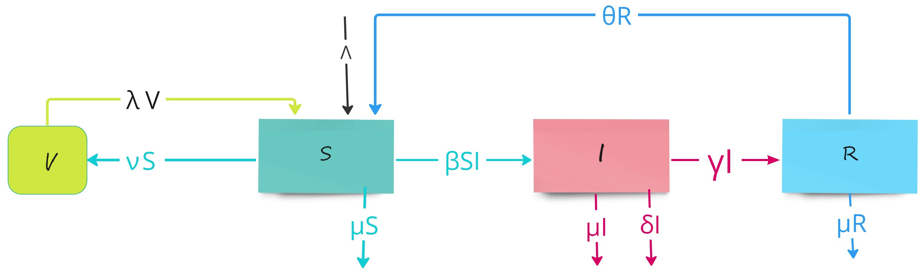
where $S\left(t\right)$, $I\left(t\right)$, $R\left(t\right)$, $V\left(t\right)$ represent the proportions of susceptible, infected, recovered, and vaccinated individuals, respectively. The function $T(·,·)$ is defined in Equation (19) below and the flowchart of the SIRVS model will be shows in Figure 1.

Kermack Mckendrick’s classic SIR model is the basis of almost all models [36], which has been widely developed recently by Sun et al. [37], in light of the effects of isolation and medical resources on the spread of COVID-19 with a fluctuating total population, and by Zhang and Zhang [38] and the references therein for the SIQS epidemic model and its related deterministic epidemic model.

Here, the time horizon can be considered infinite due to the nature of the disease, like COVID-19 or the flu that stay forever; for other, recent research papers related to epidemic models, we refer to the recent paper [26].

The parameters involved in the system (18) can be interpreted as follows:

• $\mathsf{\Lambda }$ is the constant migration rate of the susceptible population.
• $\beta \left(t\right)$ represents the transmission rate between S and I at time t.
• $\nu$ denotes the rate at which immunity decreases for vaccinated individuals.
• $\mu$ represents the natural death rate of the S, I, V, and R compartments and $\mu >0$.
• $\lambda \left(t\right)$ represents the proportional coefficient of vaccinated individuals among those susceptible at time t.
• $\theta$ signifies the rate at which recovered individuals lose their immunity and revert to being susceptible.
• $h_1$ is introduced to turn off/on the control in “summer”/“rest of the year”. See below for more details.
• ${\sigma }_i$ for $i=1,2,3$ represents the noise for the suspected, infected, and recovered people, where these parameters can be estimated from the data of the history of the epidemic. The uncertainty comes from the fact that there are infected non-detected and also recovered non-detected. For the vaccination, the uncertainty comes from the imperfect type of vaccination that could be used.
• $\gamma$ represents the constant recovery rate for the disease-infected individual.
• $\delta$ is the death rate due to disease.

The controls are given by:

• $u_1$: Represents the government’s efforts in border protection (airports and ports to track) as well as awareness campaigns and guidance.
• $u_2$: Represent the control over the number of vaccinated people

For a given $\alpha >0$, we set

$$h_1\left(x\right)=\left\{\begin{array}{cc}0\hfill & \mathrm{if}x>\alpha \hfill \\ 1\hfill & \mathrm{elsewhere}\hfill \end{array}\right.$$

The idea behind this form of $h_1$ is that the government halts additional expenditure on vaccination if the optimal cost exceeds a specified threshold $\alpha$. This threshold represents a limit beyond which the government cannot allocate further funds.

The proposed objective functional is stated as follows

$$J(s,x;u)=\mathbb{E}\left[{\int }_s^{\infty }\left(I\left(t\right)-V\left(t\right)+\frac{A}{2}{\left(u_1\left(t\right)\right)}^2+\frac{C}{2}{\left(u_2\left(t\right)\right)}^2\right)dt\right],$$

where the positive cost coefficients A and C are chosen to equate the importance of $u_1\left(t\right)$ and $u_2\left(t\right)$ at a given time. Our goal is to find the optimal controls $u_1^{*},u_2^{*}$ that minimize the cost function, i.e.,

$$J(s,x;u)\ge J(s,x;u^{*}):=T(s,x)\forall u\in U.$$

(19)

The control set is given by:

$$\begin{array}{c}\hfill U=\{u\left(t\right):=(u_1\left(t\right),u_2\left(t\right)):0\le u_i\left(t\right)\le 1,\mathrm{for}i=1,2\mathrm{and}t\in [s,T]\},\end{array}$$

(20)

By the change in variable ${\tilde{u}}_1:=\sqrt{A}{u}_1$ and ${\tilde{u}}_2:=\sqrt{C}{u}_2$, the system (18)–(19) can be written in general by setting $X\left(t\right)=(S\left(t\right),I\left(t\right),R\left(t\right),V\left(t\right))\in {\mathbb{R}}_{+}^4$ as

$$d{X}_t=\left(f\left(t,X_t\right)+h\left(T(t,x)\right){\tilde{u}}_t\right)dt+\sigma d{W}_t,X_s=x\in {\mathbb{R}}_{+}^4$$

with the cost function

$$J(s,x;\tilde{u})=\mathbb{E}\left[{\int }_s^{\infty }\left(K(t,X_t)+\frac{|{\tilde{u}}_t{|}^2}{2}\right)dt\right],\tilde{u}=({\tilde{u}}_1,{\tilde{u}}_2),$$

and $T(s,x)={inf}_{\tilde{u}}J(s,x;\tilde{u}).$

In this formulation, W is a four-dimensional Brownian motion and $\sigma$ is a $4\times 4$ matrix.

Set

$$R(a,s,x)=\left((f-ah\left(T\right)){\partial }_{x}T+\frac{1}{2}\mathrm{Tr}\left(\sigma {\sigma }^{*}\right){\partial }_{xx}^{2}T+K\right)(s,x)-\frac{a^2}{2}.$$

Hamilton–Jacobi–Bellman (HJB) equation reads

$$0={\partial }_{s}T(s,x)+\underset{a}{sup}R(a,s,x)$$

(21)

$$R^{\prime }\left(a\right)=0\mathrm{implies}\mathrm{that}h(T(s,x){\partial }_{x}T(s,x)+a=0,$$

hence

$$a^{*}(s,x)=-h\left(T(s,x)\right){\partial }_{x}T(s,x)\mathrm{and}\underset{a}{sup}R(a,s,x)=R(a^{*}(s,x),s,x)$$

Substituting in (21), we obtain:

$$\begin{array}{c}\hfill \left({\partial }_{s}T+f{\partial }_{x}T+\frac{1}{2}{\left(h\left(T\right){\partial }_{x}T\right)}^2+\frac{1}{2}\left(\mathrm{Tr}\left(\sigma {\sigma }^{*}\right){\partial }_{xx}^{2}T\right)+K\right)(s,x)=0.\end{array}$$

(22)

In this problem, we want to minimize the infection and maximize the vaccination under minimal energy $u^2.$

By the non-linear Feynman–Kac formula, the PDF (22) is interpreted by means of the coupled forward–backward stochastic system described below:

• A four-dimensional diffusion of the form

  $$d{X}_t=f(t,X_t)dt+\sigma d{W}_t,t\in [s,\infty ),$$
  Here, $\sigma$ is a positive constant for simplicity.
• A QBSDE with measurable coefficients.

  $$d{Y}_t=-{\displaystyle \frac{1}{2}}\left(K(t,X_t)+\frac{1}{2}{h}^2\left(Y_t\right){\sigma }^{-1}{Z}_t^2\right)dt+Z_{t}d{W}_t.$$

  (23)

According to Remark 2, Equation (23) has a unique solution if the stochastic process ${\left(K(t,X_t)\right)}_{t\ge 0}$ is bounded and belongs to $L^1([0,\infty )\times \Omega )$ and the function $h^2(·)$ in bounded and integrable.

5. Conclusions

In this work, we explored properties of the existence and uniqueness of one-dimensional QBSDEs in the context of an infinite time horizon. The terminal condition was assumed to be merely square integrable, and the generator or the drift term took the form of ${f\left(y\right)\left|z\right|}^2$, with f being globally integrable over the whole space $\mathbb{R}$. However, when the generator had the structure ${\eta }_{·}+f\left(y\right){\left|z\right|}^2$, where ${\eta }_{·}$ was a progressively measurable process assumed to be bounded and integrable over $[0,\infty )$, an additional condition, namely the boundedness of f, was sufficient to ensure the well posedness of the problem. To this end, we made use of mathematical analysis and probabilistic techniques, namely Krylov’s type estimates for functionals of the solution and Itô–Krylov’s formula for a specific class of BSDEs with singular drifts. As the main tool, we used a phase-space change in the variable known as the Zvonkin transformation to eliminate the whole singular term.

We also established a comparison theorem as part of our analysis for a class of infinite time horizon QBSDEs having irregular drifts. As an application, we demonstrated the existence and uniqueness of viscosity solutions for a related class of QPDEs with irregular, merely measurable, and integrable coefficients. Particularly, we derived a probabilistic representation of the solution for QPDEs with measurable coefficients. Additionally, we explored an example involving an epidemic model that could be solved using infinite time horizon QBSDEs with irregular generators.

For our future research, we plan to analyze and establish probabilistic representations of solutions for partial integral differential equations of a quadratic nature with irregular coefficients. This will be achieved by utilizing solutions from a specific class of QBSDEs with jumps, where the noise arises from a combination of Brownian motion and an independent Poisson process.

References

- Bismut, J.M. Contrôle des Systemes LinéAires Quadratiques: Applications de l’Intégrale Stochastique; Springer: Berlin/Heidelberg, Germany, 1978. [Google Scholar]
- Pardoux, E.; Peng, S. Adapted solution of a backward stochastic differential equation. Syst. Control Lett. 1990, 14, 55–61. [Google Scholar] [CrossRef]
- Pardoux, E. Generalized discontinuous backward stochastic differential equations. In Pitman Research Notes in Mathematics Series; Longman: London, UK, 1997; pp. 207–219. [Google Scholar]
- Pardoux, E.; Zhang, S. Generalized BSDEs and nonlinear Neumann boundary value problems. Probab. Theory Relat. Fields 1998, 110, 535–558. [Google Scholar] [CrossRef]
- Darling, R.W.; Pardoux, E. Backwards SDE with random terminal time and applications to semilinear elliptic PDE. Ann. Probab. 1997, 25, 1135–1159. [Google Scholar] [CrossRef]
- Peng, S. Probabilistic interpretation for systems of quasilinear parabolic partial differential equations. Stochastics Stochastics Rep. 1991, 37, 61–74. [Google Scholar]
- Chen, Z. Existence and uniqueness for BSDE with stopping time. Chin. Sci. Bull. 1998, 43, 96–99. [Google Scholar] [CrossRef]
- Chen, Z.; Wang, B. Infinite time interval BSDEs and the convergence of g-martingales. J. Aust. Math. Soc. 2000, 69, 187–211. [Google Scholar] [CrossRef]
- Rouge, R.; El Karoui, N. Pricing via utility maximization and entropy. Math. Financ. 2000, 10, 259–276. [Google Scholar] [CrossRef]
- El Karoui, N.; Peng, S.; Quenez, M.C. Backward stochastic differential equations in finance. Math. Financ. 1997, 7, 1–71. [Google Scholar] [CrossRef]
- Ankirchner, S.; Fromm, A.; Hu, Y.; Imkeller, P.; Muller, M.; Popier, A.; Dos Reis, G. On cross hedging, BSDE and Malliavin’s calculus. Ann. Appl. Probab. 2005, 15, 1691–1712. [Google Scholar]
- Briand, P.; Confortola, F. Quadratic BSDEs with random terminal time and elliptic PDEs in infinite dimension. Electron. J. Probab. 2008, 13, 1529–1561. [Google Scholar]
- Kobylanski, M. Backward stochastic differential equations and partial differential equations with quadratic growth. Ann. Probab. 2000, 28, 558–602. [Google Scholar] [CrossRef]
- Ekren, I.; Nadtochiy, S. Utility-based pricing and hedging of contingent claims in Almgren-Chriss model with temporary price impact. Math. Financ. 2022, 32, 172–225. [Google Scholar] [CrossRef]
- Dermoune, A.; Hamadène, S.; Ouknine, Y. Backward stochastic differential equation with local time. Stochastics Stoch. Rep. 1999, 66, 103–119. [Google Scholar] [CrossRef]
- Barrieu, P.; El Karoui, N. Monotone stability of quadratic semimartingales with applications to unbounded general quadratic BSDEs. Ann. Probab. 2013, 41, 1831–1863. [Google Scholar] [CrossRef]
- Briand, P.; Hu, Y. BSDE with quadratic growth and unbounded terminal value. Probab. Theory Relat. Fields 2006, 136, 604–618. [Google Scholar] [CrossRef]
- Lepeltier, J.P.; San Martin, J. Existence for BSDE with superlinear-quadratic coefficient. Stochastics Int. J. Probab. Stoch. Process. 1998, 63, 227–240. [Google Scholar] [CrossRef]
- Lepeltier, J.P.; Xu, M. Penalization method for reflected backward stochastic differential equations with one rcll barrier. Stat. Probab. Lett. 2005, 75, 58–66. [Google Scholar] [CrossRef]
- Tevzadze, R. Solvability of backward stochastic differential equations with quadratic growth. Stoch. Process. Their Appl. 2008, 118, 503–515. [Google Scholar] [CrossRef]
- Bahlali, K.; Eddahbi, M.; Ouknine, Y. Solvability of some quadratic BSDEs without exponential moments. Comptes Rendus Mathématiques 2013, 351, 229–233. [Google Scholar] [CrossRef]
- Bahlali, K.; Eddahbi, M.; Ouknine, Y. Quadratic BSDE with L2-terminal data: Krylov’s estimate, Itô-Krylov’s formula and existence results. Ann. Probab. 2017, 45, 2377–2397. [Google Scholar] [CrossRef]
- Zvonkin, A.K. A transformation of the phase space of a diffusion process that removes the drift. Math. USSR-Sb. 1974, 22, 129–149. [Google Scholar] [CrossRef]
- Hamadène, S.; Lepeltier, J.P.; Wu, Z. Infinite horizon reflected backward stochastic differential equations and applications in mixed control and game problems. Probab. Math. Stat. 1999, 19, 211–234. [Google Scholar]
- Peng, S.; Shi, Y. Infinite horizon forward-backward stochastic differential equations. Stoch. Process. Their Appl. 2000, 85, 75–92. [Google Scholar] [CrossRef]
- Freddi, L.; Goreac, D. Infinite horizon optimal control of a SIR epidemic under an ICU constraint. arXiv 2023, arXiv:2306.10513. [Google Scholar]
- Bergomi, L. Stochastic Volatility Modeling; CRC Press: Boca Raton, FL, USA, 2015. [Google Scholar]
- Cruz, J.; Grossinho, M.; Sevcovic, D.; Udeani, C.I. Linear and Nonlinear Partial Integro-Differential Equations arising from Finance. arXiv 2022, arXiv:2207.11568. [Google Scholar]
- Düring, B.; Jüngel, A. Existence and uniqueness of solutions to a quasilinear parabolic equation with quadratic gradients in financial markets. Nonlinear Anal. Theory Methods Appl. 2005, 62, 519–544. [Google Scholar] [CrossRef]
- Shi, Y.; Zhao, H. Forward-backward stochastic differential equations on infinite horizon and quasilinear elliptic PDEs. J. Math. Anal. Appl. 2020, 485, 123791. [Google Scholar] [CrossRef]
- El Karoui, N.; Kapoudjian, C.; Pardoux, E.; Peng, S.; Quenez, M.C. Reflected solutions of backward SDE’s, and related obstacle problems for PDE’s. Ann. Probab. 1997, 25, 702–737. [Google Scholar] [CrossRef]
- Crandall, M.G.; Lions, P.L. Viscosity solutions of Hamilton-Jacobi equations. Trans. Am. Math. Soc. 1983, 277, 1–42. [Google Scholar] [CrossRef]
- Peng, S. Monotonic limit theorem of BSDE and nonlinear decomposition theorem of Doob–Meyer’s type. Probab. Theory Relat. Fields 1999, 113, 473–499. [Google Scholar] [CrossRef]
- Bensoussan, A.; Peng, S. Singular perturbations in optimal control problems. Autom.-Prod. Inform. Ind. 1986, 20, 359–381. [Google Scholar]
- Bensoussan, A. Perturbation Methods in Optimal Control, 1st ed.; Wiley: Hoboken, NJ, USA, 1988. [Google Scholar]
- Kermack, W.O.; McKendrick, A.G. A contribution to the mathematical theory of epidemics. Proc. R. Soc. Lond. Ser. A 1927, 115, 700–721. [Google Scholar]
- Sun, G.Q.; Wang, S.F.; Li, M.T.; Li, L.; Zhang, J.; Zhang, W.; Jin, Z.; Feng, G.L. Transmission dynamics of COVID-19 in Wuhan, China: Effects of lockdown and medical resources. Nonlinear Dyn. 2020, 101, 1981–1993. [Google Scholar] [CrossRef] [PubMed]
- Zhang, X.B.; Zhang, X.H. The threshold of a deterministic and a stochastic SIQS epidemic model with varying total population size. Appl. Math. Model. 2021, 91, 749–767. [Google Scholar] [CrossRef]
Figure 1.
The flowchart of the SIRVS model.
Disclaimer/Publisher’s Note: The statements, opinions and data contained in all publications are solely those of the individual author(s) and contributor(s) and not of MDPI and/or the editor(s). MDPI and/or the editor(s) disclaim responsibility for any injury to people or property resulting from any ideas, methods, instructions or products referred to in the content. |
© 2023 by the authors. Licensee MDPI, Basel, Switzerland. This article is an open access article distributed under the terms and conditions of the Creative Commons Attribution (CC BY) license (https://creativecommons.org/licenses/by/4.0/).
Share and Cite
MDPI and ACS Style
Eddahbi, M.; Kebiri, O.; Sene, A. Infinite Horizon Irregular Quadratic BSDE and Applications to Quadratic PDE and Epidemic Models with Singular Coefficients. Axioms 2023, 12, 1068. https://doi.org/10.3390/axioms12121068
AMA Style
Eddahbi M, Kebiri O, Sene A. Infinite Horizon Irregular Quadratic BSDE and Applications to Quadratic PDE and Epidemic Models with Singular Coefficients. Axioms. 2023; 12(12):1068. https://doi.org/10.3390/axioms12121068
Chicago/Turabian StyleEddahbi, Mhamed, Omar Kebiri, and Abou Sene. 2023. "Infinite Horizon Irregular Quadratic BSDE and Applications to Quadratic PDE and Epidemic Models with Singular Coefficients" Axioms 12, no. 12: 1068. https://doi.org/10.3390/axioms12121068
Note that from the first issue of 2016, this journal uses article numbers instead of page numbers. See further details here.