Higher-Order Benjamin–Ono Model for Ocean Internal Solitary Waves and Its Related Properties

Abstract

In this study, the propagation of internal solitary waves in oceans at great depths was analyzed. Using multi-scale analysis and perturbation expansion, the basic equation is simplified to the classical Benjamin–Ono equation with variable coefficients. To better describe the propagation characteristics of solitary waves, we derived a higher-order variable-coefficient integral differential (Benjamin–Ono) equation. Subsequently, the bilinear form of the model was derived using Hirota’s bilinear method, and a multi-soliton solution was obtained. Based on the multi-soliton solution of the model, we further studied the interaction of the soliton, which led to the discovery of Mach reflection. Some conclusions were drawn, which are of potential value for further study of solitary waves in the ocean.

1. Introduction

An internal wave is an important type of seawater movement that is not only an important part of transferring large-scale and medium-scale motion energy, but also an important reason for seawater mixing and the formation of fine structures [1,2,3,4]. An internal wave is an internal wave of a marine water body with stable density stratification. It is a type of heavy ocean internal wave or an internal inertial gravity wave [5,6,7]. The fluctuation is very slow, with a phase speed of less than 1 m/s. Typical internal waves have amplitudes of several meters to dozens of meters, wavelengths of nearly 100 m to dozens of kilometers, and periods of several minutes to dozens of hours. These factors are crucial in explaining the mixing of seawater and the formation of fine structures. Internal waves are an important movement of seawater, which not only transfer energy from the upper layer of the ocean to the deep layer, but also bring colder deep-sea water together with nutrients to the warmer shallow layer to promote the growth and reproduction of organisms [8,9,10]. The internal wave causes fluctuations in the equal-density surface; this changes the magnitude and direction of the sound velocity and has a significant influence on the sonar, which is beneficial to the concealment of the submarine underwater, but detrimental to offshore facilities [11,12].

As a common marine dynamic phenomenon that occurs in dense stratified seawater [13,14], internal solitary waves are often found in the South China Sea [15], Sulu Sea [16], Andaman Sea [17] and other continental shelf edge waters, and they are very extensive in parts of the Earth. Internal solitary waves usually propagate in the form of wave groups, and their characteristic wavelengths range from hundreds of meters to more than ten kilometers. The typical distance between wave packets ranges from tens of kilometers to 100 km [18,19]. It is not only an important part of the marine energy cascade but also one of the key physical processes that affect marine productivity; it has an important impact on the development of marine resources, marine engineering, the marine ecological environment, and fisheries. Hence, the study of internal solitary waves is significantly important [20,21].

The KdV equation is typically used to describe the internal solitary wave. KdV is generated when studying waves in shallow water [22,23,24]. Keulegan [25] and Long [26] were the first to discover internal solitary waves that could propagate in two liquids of different densities. A general theoretical treatment of a new class of finite-amplitude long-standing waves was presented by Benjamin [27,28]. Benney [29] studied a finite-amplitude wave in an inviscid fluid. Benjamin [28] and Ono [30] obtained the well-known BO equation by studying stratified fluids at large depths:

$$\begin{array}{c}\hfill f_t+\alpha f{f}_x-\beta {\left[\aleph \left(f\right)\right]}_{xx}=0,\end{array}$$

(1)

where $\alpha$ and $\beta$ are constants, ℵ denotes Hilbert transform of f. Later, Joseph and Kubota et al. further studied the character of internal gravity waves in both the shallow and deep fluid, and obtained the intermediate long-wave (ILW) equation:

$$\begin{array}{c}\hfill f_t+2f{f}_x+G\left[f_{xx}\right]=0,\end{array}$$

(2)

where $G\left[f(x,t)\right]=\frac{1}{2}\lambda {\int }_{-\infty }^{+\infty }coth\frac{1}{2}\pi \lambda (x^{\prime }-x)f(x,t)d{x}^{\prime },$ and ${\lambda }^{-1}$ denotes the depth of the fluid. ILW equation represents the natural connection between the Korteweg–de Vries shallow water and Benjamin–Ono deep water theories.

Recently, with significant progress in research, researchers have gradually shifted their attention from low- to high-order models [31,32,33,34,35]. Grimshaw et al. [36] investigated internal solitary waves in density- and current-layered shear flows with free surfaces, leading to the derivation of higher-order KdV equations. Kaya et al. [37] obtained the exact solitary wave solution and the numerical solution of the fifth-order KdV equation under initial conditions. Duffy et al. [38] obtained an explicit traveling solitary wave solution for a seventh-order generalized KdV equation. Craig et al. [39] proposed a higher-order BO model for internal waves in a two-layer ocean with two distinct but constant densities. In addition to this, Germán Foneca and Felipe Linares [40] showed existence and uniqueness of global solutions for the lower-order BO equation. Hidekazu Tsuji and Masayuki Oikawa [41] numerically solved the lower-order BO equation describing internal solitary waves and observed that Mach reflection occurs at small incidence angles. However, several studies have been conducted on higher-order BO equations describing internal solitary waves. With the advancement of research, it is imperative to explore higher-order BO equations in order to more scientifically and accurately describe physical phenomena in nature. Accordingly, we used a new perturbation expansion and multiscale analysis method to deduce the higher-order BO equation and study its properties.

The occurrence of Mach reflection arises from the interaction between a barrier and a sufficiently large amplitude line soliton or classical shock at an acute angle. A Y-shaped triad is formed by two smaller amplitude solitons or shocks and a larger “Mach” stem perpendicular to the barrier. This phenomenon was first experimentally reported in J. Scott Russell’s seminal paper [42], which studied shallow water solitons impinging on a corner. Later, Ernst Mach observed his eponymous phenomenon arising from interacting shocks in gas dynamics [43,44]. We investigate the Mach reflection of the higher-order BO equation.

In this study, a new higher order Benjamin-Ono equation was obtained for an internal solitary wave. The remainder of this paper is organized as follows: In Section 2, we derive the well-known Benjamin–Ono (BO) model. In Section 3, based on the new perturbation expansion and multiscale analysis, the higher order Benjamin–Ono equation is obtained for the first time. In Section 4, the bilinear form and multi-soliton solutions of the higher order Benjamin–Ono equation are studied using Hirota’s bilinear method [45,46]. And we study the interaction of solitons, determine the phenomenon of Mach reflection, and draw conclusions. Finally, a summary is presented in Section 5.

2. Derivation of BO Equation

We considered the two-dimensional motion of two layers of incompressible and finite-depth fluids stratified by density in the y direction. The governing equations are as follows:

$$\left\{\begin{array}{c}\frac{\partial u}{\partial x}+\frac{\partial v}{\partial y}=0,\hfill \\ \frac{\partial \rho }{\partial t}+u\frac{\partial \rho }{\partial x}+v\frac{\partial \rho }{\partial y}=0,\hfill \\ \rho \left(\frac{\partial u}{\partial t}+u\frac{\partial u}{\partial x}+v\frac{\partial u}{\partial y}\right)=-\frac{\partial p}{\partial x},\hfill \\ \rho \left(\frac{\partial v}{\partial t}+u\frac{\partial v}{\partial x}+v\frac{\partial v}{\partial y}\right)=-\frac{\partial p}{\partial y}-g\rho ,\hfill \end{array}\right.$$

(3)

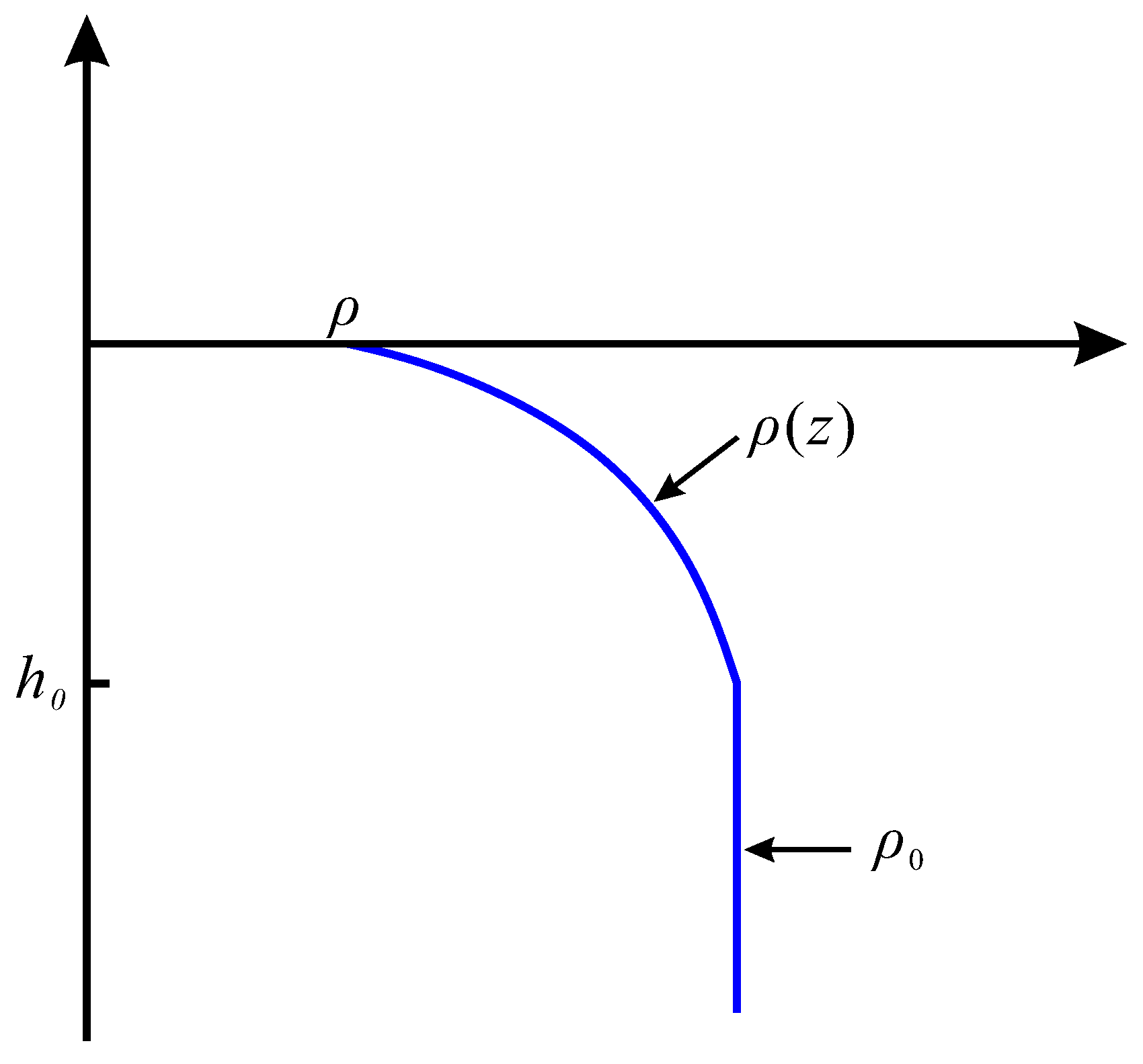
where u and v are the velocity components in the directions x and y, $\rho$ is the density, t is the time variable, and p is the fluid pressure. g is the acceleration due to gravity, and the basic hydrostatic balance is $\frac{d{p}_0}{dy}=-g{\rho }_0$. The appropriate boundary conditions associated with $v\left(y\right)$ are $v=0$ at $y=0$ and $v\to 0$ at $y\to \infty$. We assume that the density is continuous at $y=h_0$. At $h_0\ge y\ge 0$, the density ${\rho }_0\left(y\right)$ varies with y; however, at $y\ge h_0$, it remains constant.

$$\rho =\left\{\begin{array}{c}{\rho }_0\left(y\right),h_0\ge y\ge 0,\hfill \\ {\rho }_0(=constant),y\ge h_0.\hfill \end{array}\right.$$

(4)

That is, the density of the upper layer of the fluid changes with the change of y, and the density of the lower layer does not change (see Figure 1).

The boundary conditions for $v\left(y\right)$ are: $v=0$ when $y=0$ and $y=h_1$. Further, we study the wave equation by matching the upper and lower solutions at $y=h_0$ using coordinate transformation and perturbation methods.

Considering the case $h_0\ge y\ge 0$. Introducing the following transformations:

$$T_1={ϵ}^{2}t,T_2={ϵ}^{3}t,X=ϵ\left(x-t\right),$$

(5)

that is

$$\begin{array}{c}\hfill \frac{\partial }{\partial t}=-ϵ\frac{\partial }{\partial X}+{ϵ}^2\frac{\partial }{\partial T_1}+{ϵ}^3\frac{\partial }{\partial T_2},\frac{\partial }{\partial x}=ϵ\frac{\partial }{\partial X},\frac{\partial }{\partial y}=ϵ\frac{\partial }{\partial y}.\end{array}$$

Assuming that $u,v,c,p$ and $\rho$ have the following asymptotic expansion, we obtain:

$$\left\{\begin{array}{c}u\left(X,y,T_1,T_2\right)=ϵu_1\left(X,y,T_1,T_2\right)+{ϵ}^2{u}_2\left(X,y,T_1,T_2\right)+{ϵ}^3{u}_3\left(X,y,T_1,T_2\right)+\cdots ,\hfill \\ v\left(X,y,T_1,T_2\right)={ϵ}^2{v}_1\left(X,y,T_1,T_2\right)+{ϵ}^3{v}_2\left(X,y,T_1,T_2\right)+{ϵ}^4{v}_3\left(X,y,T_1,T_2\right)+\cdots ,\hfill \\ p\left(X,y,T_1,T_2\right)=\hfill \\ p_0\left(y\right)+ϵp_1\left(X,y,T_1,T_2\right)+{ϵ}^2{p}_2\left(X,y,T_1,T_2\right)+{ϵ}^3{p}_3\left(X,y,T_1,T_2\right)+\cdots ,\hfill \\ \rho \left(X,y,T_1,T_2\right)=\hfill \\ {\rho }_0\left(y\right)+ϵ{\rho }_1\left(X,y,T_1,T_2\right)+{ϵ}^2{\rho }_2\left(X,y,T_1,T_2\right)+{ϵ}^3{\rho }_3\left(X,y,T_1,T_2\right)+\cdots .\hfill \end{array}\right.$$

(6)

where a small parameter $ϵ\ll 1$ represents the nonlinear strength.

By substituting the Equations (5) and (6) into Equation (3), the lowest-order approximation equation for $ϵ$ is

$$\left\{\begin{array}{c}\frac{\partial u_1}{\partial X}+\frac{\partial v_1}{\partial y}=0,\hfill \\ -\frac{\partial {\rho }_1}{\partial X}+v_1\frac{d{\rho }_0}{dy}=0,\hfill \\ -{\rho }_0\frac{\partial u_1}{\partial X}+\frac{\partial p_1}{\partial X}=0,\hfill \\ \frac{\partial p_1}{\partial y}=-g{\rho }_1.\hfill \end{array}\right.$$

(7)

By eliminating $p_1,u_1$ and ${\rho }_1$, we obtain the governing equation for $v_1$:

$$\begin{array}{c}\hfill \frac{\partial }{\partial y}\left[{\rho }_0\left(y\right)\frac{\partial v_1}{\partial y}\right]-g{v}_1\frac{d{\rho }_0\left(y\right)}{dy}=0.\end{array}$$

(8)

By separating the variables, we assume that the solution of Equation (8) has the following form:

$$v_1\left(X,y,T_1,T_2\right)=-\varphi \left(y\right)f_X\left(X,T_1,T_2\right).$$

(9)

$$\begin{array}{c}\hfill \frac{\partial }{\partial y}\left[{\rho }_0\left(y\right)\frac{d\varphi }{dy}\right]-\frac{g}{c_0^2}\varphi \frac{d{\rho }_0}{dy}=0,\end{array}$$

(10)

Substituting Equation (9) into Equation (7), we obtain

$$\begin{array}{c}\hfill u_1=f\frac{d\varphi }{dy},p_1={\rho }_0\frac{d\varphi }{dy}f,{\rho }_1=-\varphi \frac{d{\rho }_0\left(y\right)}{dy}f.\end{array}$$

(11)

Furthermore, we obtain the following next-order approximate equation for $ϵ$:

$$\left\{\begin{array}{c}\frac{\partial u_2}{\partial X}+\frac{\partial v_2}{\partial y}=0,\hfill \\ -\frac{\partial {\rho }_2}{\partial X}+v_2\frac{d{\rho }_0}{dy}=A_1=-v_1\frac{\partial {\rho }_1}{\partial y}-\frac{\partial {\rho }_1}{\partial T_1}-u_1\frac{\partial {\rho }_1}{\partial X},\hfill \\ -{\rho }_0\frac{\partial u_2}{\partial X}+\frac{\partial p_2}{\partial X}=A_2\hfill \\ =-{\rho }_0{u}_1\frac{\partial u_1}{\partial X}-{\rho }_0{v}_1\frac{\partial u_1}{\partial y}-{\rho }_0\frac{\partial u_1}{\partial T_1}+{\rho }_1\frac{\partial u_1}{\partial X}-{\rho }_1\left({\rho }_0\frac{\partial u_1}{\partial X}-\frac{\partial P_1}{\partial X}\right),\hfill \\ \frac{\partial p_2}{\partial y}=-g{\rho }_2.\hfill \end{array}\right.$$

(12)

Similarly, the governing equation of $v_2$ is

$$\begin{array}{c}\hfill \frac{\partial }{\partial y}\left[{\rho }_0\left(y\right)\frac{\partial v_2}{\partial y}\right]-g{v}_2\frac{d{\rho }_0}{dy}=\frac{\partial A_2}{\partial y}-g{A}_1.\end{array}$$

(13)

By multiplying both sides of Equation (13) by $\varphi$ and integrating y from 0 to $h_0$, we obtain

$$\begin{array}{c}\hfill {\int }_0^{h_0}\left[\frac{\partial }{\partial y}\left({\rho }_0\frac{\partial v_2}{\partial y}\right)-g\frac{d{\rho }_0}{dy}{v}_2\right]\varphi dy={\int }_0^{h_0}\left(a_1{f}_{T_1}+a_{2}f{f}_X\right)\varphi dy.\end{array}$$

(14)

where

$$\begin{array}{c}{a}_1=-{\rho }_0\frac{d\varphi }{dy}-{\rho }_0\frac{d^2\varphi }{d{y}^2},\hfill \\ a_2=\frac{\partial }{\partial y}\left[\left(\frac{{\rho }_0}{g}\frac{d^2\varphi }{d{y}^2}\frac{d\varphi }{dy}\right)-{\rho }_0\frac{d\varphi }{dy}\frac{d\varphi }{dy}+{\rho }_0\varphi \frac{d^2\varphi }{d{y}^2}\right]+\left(\varphi {\rho }_0\frac{d^3\varphi }{d{y}^3}-{\rho }_0\frac{d^2\varphi }{d{y}^2}-\frac{d\varphi }{dy}{\rho }_0\frac{d^2\varphi }{d{y}^2}\right).\hfill \end{array}$$

Next, we consider another case that $y\ge h_0$. Similarly, we introduce the transformations $T={ϵ}^{2}t$ and $X=x-t$: $u,v,c,p$ and $\rho$ exhibit the following asymptotic expansion:

$$\left\{\begin{array}{c}u={ϵ}^{2}U\left(X,y,T,ϵ\right),\hfill \\ v={ϵ}^{2}V\left(X,y,T,ϵ\right),\hfill \\ p=p_0\left(y\right)+{ϵ}^{2}P\left(X,y,T,ϵ\right),\hfill \\ \rho ={\rho }_0\left(y\right)+{ϵ}^{4}R\left(X,y,T,ϵ\right).\hfill \end{array}\right.$$

(15)

Substituting transformations and Equation (15) into Equation (3), we obtain

$$\begin{array}{c}\hfill \frac{{\partial }^{2}V}{\partial X^2}+\frac{{\partial }^{2}V}{\partial y^2}=0.\end{array}$$

(16)

Similarly, the boundary conditions of V are

$$\left\{\begin{array}{c}{\left.V\left(X,y,T,ϵ\right)\right|}_{y=h_0}\to -f_X{\left.\varphi \left(y\right)\right|}_{y=h_0},\hfill \\ V\left(X,y,T,ϵ\right)\to 0,y\to \infty .\hfill \end{array}\right.$$

(17)

we obtain the solutions to Equation (16) as follows:

$$\begin{array}{c}\hfill V\left(X,y,T,ϵ\right)=\frac{P.V.}{\pi }{\int }_{-\infty }^{+\infty }-f_X\left(X^{\prime },T_1,ϵ\right)\frac{y-h_0}{{\left(y+h_0\right)}^2+{\left(X-X^{\prime }\right)}^2}d{X}^{\prime },\end{array}$$

(18)

where $P.V.$ denotes the principal value of the Cauchy integral. Differentiating Equation (18) with respect to y.

$$\frac{\partial V(X,y,T,ϵ)}{\partial y}=\frac{1}{\pi }P.V.{\int }_{-\infty }^{+\infty }-f_X\left(X^{\prime },T_1,ϵ\right)\frac{{\left(X-X^{\prime }\right)}^2-{\left(y-h_0\right)}^2}{{\left[{\left(y-h_0\right)}^2+{\left(X-X^{\prime }\right)}^2\right]}^2}d{X}^{\prime }.$$

(19)

The two cases $h_0\ge y\ge 0$ and $y\ge h_0$ have been deduced. Finally, we match them at $y=h_0$. Assuming that the solutions of the two regions are continuous at $y=h_0$, we obtain

$${ϵ}^2{v}_1\left(X,h_0,T_1\right)+{ϵ}^3{v}_2\left(X,h_0,T_1\right)={ϵ}^{2}V\left(X,h_0,T,ϵ\right),$$

(20)

$$\frac{\partial \left({ϵ}^2{v}_1\left(X,h_0,T_1\right)+{ϵ}^3{v}_2\left(X,h_0,T_1\right)\right)}{\partial y}=\frac{\partial \left({ϵ}^{2}V\left(X,h_0,T,ϵ\right)\right)}{\partial y}.$$

(21)

Combining Equation (20), we obtain

$$\varphi \left(h_0\right)\frac{\partial f(X,T_1)}{\partial X}=V\left(X,h_0,T\right),v_2(X,h_0,T_1)=0.$$

(22)

Based on Equation (19), we obtain

$$\frac{\partial V(X,h_0,T,ϵ)}{\partial y}=\frac{ϵ}{\pi }P.V.\frac{{\partial }^2}{\partial X^2}{\int }_{-\infty }^{+\infty }\frac{f(X^{\prime },T_1)}{X-X^{\prime }}d{X}^{\prime }.$$

(23)

From Equations (21) and (23), we obtain

$$\begin{array}{c}\hfill \frac{d\varphi \left(h_0\right)}{dy}=0,\frac{\partial v_2(X,h_0,T_1)}{\partial y}=\frac{1}{\pi }P.V.\frac{{\partial }^2}{\partial X^2}{\int }_{-\infty }^{+\infty }\frac{f(X^{\prime },T_1)}{X-X^{\prime }}d{X}^{\prime }.\end{array}$$

(24)

Further, substituting Equations (22) and (24) into Equation (14), we obtain a new governing equation:

$$\begin{array}{c}\hfill f_{T_1}+a_1^{\prime }f{f}_X+a_2^{\prime }{\left[\aleph \left(f\right)\right]}_{XX}=0.\end{array}$$

(25)

where

$$\begin{array}{c}{a}_1^{\prime }=\frac{{\int }_{-\infty }^{+\infty }\left\{\frac{\partial }{\partial y}\left[\left(\frac{{\rho }_0}{g}\frac{d^2\varphi }{d{y}^2}\frac{d\varphi }{dy}\right)-{\rho }_0\frac{d\varphi }{dy}\frac{d\varphi }{dy}+{\rho }_0\varphi \frac{d^2\varphi }{d{y}^2}\right]+\left(\varphi {\rho }_0\frac{d^3\varphi }{d{y}^3}-{\rho }_0\frac{d^2\varphi }{d{y}^2}-\frac{d\varphi }{dy}{\rho }_0\frac{d^2\varphi }{d{y}^2}\right)\right\}dy}{{\int }_{-\infty }^{+\infty }\left(-{\rho }_0\frac{d\varphi }{dy}-{\rho }_0\frac{d^2\varphi }{d{y}^2}\right)dy},\hfill \\ a_2^{\prime }=\frac{-{\rho }_0\left(h_0\right)\varphi \left(h_0\right)}{{\int }_{-\infty }^{+\infty }\varphi \left(-{\rho }_0\frac{d\varphi }{dy}-{\rho }_0\frac{d^2\varphi }{d{y}^2}\right)dy},\aleph \left(f\right)=\frac{1}{\pi }P.V.{\int }_{-\infty }^{+\infty }\frac{f(X^{\prime },T_1)}{X-X^{\prime }}d{X}^{\prime }.\hfill \end{array}$$

Equation (25) is a model that is used for the first time to describe internal solitary waves in the ocean. Note that when $h_0\to \infty$, Equation (25) is converted into the BO equation, which was first deduced by Benjamin [28] and Ono [30] as a model for long internal gravity waves in deep stratified fluids; and in the opposite limit, Equation (25) is converted into the KdV equation, which is first used by Long to describes Rossby waves in a single-layer barotropic fluid. It is necessary to obtain a higher-order BO equation to describe internal solitary waves in the ocean more accurately.

3. Derivation of Higher-Order BO Equation

In the domain $h_0\ge y\ge 0$, we can obtain a higher-order approximate equation for $ϵ$:

$$\left\{\begin{array}{c}\frac{\partial u_3}{\partial X}+\frac{\partial v_3}{\partial y}=0,\hfill \\ -\frac{\partial {\rho }_3}{\partial X}+v_3\frac{d{\rho }_0}{dy}=A_3,\hfill \\ -{\rho }_0\frac{\partial u_3}{\partial X}+\frac{\partial p_3}{\partial X}=A_4,\hfill \\ \frac{\partial p_3}{\partial y}+g{\rho }_3=A_5,\hfill \end{array}\right.$$

(26)

where

$$\begin{array}{c}{A}_3=-\frac{\partial {\rho }_2}{\partial T_1}-\frac{\partial {\rho }_1}{\partial T_2}-v_1\frac{\partial {\rho }_2}{\partial y}-u_1\frac{\partial {\rho }_2}{\partial X}-u_2\frac{\partial {\rho }_1}{\partial X}-v_2\frac{\partial {\rho }_1}{\partial X},A_5={\rho }_0\frac{\partial v_1}{\partial X},\hfill \\ A_4=-{\rho }_0\frac{\partial u_2}{\partial T_1}-{\rho }_0{\rho }_1\frac{\partial u_1}{\partial T_1}-{\rho }_0\frac{\partial u_1}{\partial T_2}-{\rho }_0{u}_1\frac{\partial u_2}{\partial X}-{\rho }_0{u}_2\frac{\partial u_1}{\partial X}-{\rho }_0{v}_1\frac{\partial u_2}{\partial y}-{\rho }_0{v}_2\frac{\partial u_1}{\partial y}\hfill \\ +{\rho }_1{\rho }_0\frac{\partial u_2}{\partial X}+{\rho }_1^2\frac{\partial u_1}{\partial X}-{\rho }_1\frac{\partial p_2}{\partial X}-{\rho }_1{\rho }_0{u}_1\frac{\partial u_1}{\partial X}-{\rho }_1{\rho }_0{v}_1\frac{\partial u_1}{\partial y}+{\rho }_2{\rho }_0\frac{\partial u_1}{\partial X}-{\rho }_2\frac{\partial p_1}{\partial X}.\hfill \end{array}$$

By eliminating $p_3,u_3$ and ${\rho }_3$, we obtain the governing equation and boundary conditions for $v_3$:

$$\begin{array}{c}\hfill \frac{\partial }{\partial y}\left[{\rho }_0\left(y\right)\frac{\partial v_3}{\partial y}\right]-g{v}_3\frac{d{\rho }_0}{dy}=\frac{\partial A_4}{\partial y}-\frac{\partial A_5}{\partial X}-g{A}_3.\end{array}$$

(27)

Similarly, multiplying both sides of Equation (27) by $\varphi$ and integrating y from 0 to $h_0$, we obtain

$$\begin{array}{c}\hfill {\int }_0^{h_0}\varphi \left[\frac{\partial }{\partial y}\left({\rho }_0\frac{\partial v_3}{\partial y}\right)-g\frac{d{\rho }_0}{dy}{v}_3\right]dy={\int }_0^{h_0}\varphi \left(\frac{\partial A_4}{\partial y}-\frac{\partial A_5}{\partial X}-g{A}_3\right)dy,\end{array}$$

(28)

Equation (28) can be sorted as follows:

$$\begin{array}{cc}\hfill {\int }_0^{h_0}\varphi \left[\frac{\partial }{\partial y}\left({\rho }_0\frac{\partial v_3}{\partial y}\right)-g\frac{d{\rho }_0}{dy}{v}_3\right]dy& ={\int }_0^{h_0}\varphi \left(b_1^{\prime }{f}_{T_2}+b_2^{\prime }{f}_{XXX}+b_3^{\prime }{f}^2{f}_X+b_4^{\prime }{f}_X\aleph {\left(f\right)}_X\right.\hfill \\ & \left.+b_5^{\prime }\aleph {\left(f{f}_X\right)}_X+b_6^{\prime }f\aleph {\left(f\right)}_{XXX}\right)dy.\hfill \end{array}$$

(29)

where

$$\begin{array}{c}{b}_1^{\prime }=-\frac{d\varphi }{dy}\frac{d{\rho }_0}{dy}-{\rho }_0\frac{d^2\varphi }{d{y}^2},\hfill \\ b_2^{\prime }=\frac{\partial }{\partial y}\left({\rho }_0\frac{{\int }_{-\infty }^{+\infty }\left\{\frac{\partial }{\partial y}\left[\left(\frac{{\rho }_0}{g}\frac{d^2\varphi }{d{y}^2}\frac{d\varphi }{dy}\right)-{\rho }_0\frac{d\varphi }{dy}\frac{d\varphi }{dy}+{\rho }_0\varphi \frac{d^2\varphi }{d{y}^2}\right]+\left(\varphi {\rho }_0\frac{d^3\varphi }{d{y}^3}-{\rho }_0\frac{d^2\varphi }{d{y}^2}-\frac{d\varphi }{dy}{\rho }_0\frac{d^2\varphi }{d{y}^2}\right)\right\}dy}{{\int }_{-\infty }^{+\infty }\left(-{\rho }_0\frac{d\varphi }{dy}-{\rho }_0\frac{d^2\varphi }{d{y}^2}\right)dy}\right),\hfill \\ b_3^{\prime }=\frac{\partial }{\partial y}\left[\frac{{\rho }_0^2}{g}{\left(\frac{d\varphi }{dy}\right)}^2\frac{a_2^{\prime }}{a_1}\right]-\frac{{\rho }_0}{g}\frac{d\varphi }{dy}\left[\frac{{\rho }_0}{g}{\left(\frac{d\varphi }{dy}\right)}^2+{\rho }_0{\left(\frac{d\varphi }{dy}\right)}^2-{\rho }_0\varphi \frac{d^2\varphi }{d{y}^2}\right],\hfill \\ b_4^{\prime }=\frac{\partial }{\partial y}\left[\frac{{\rho }_0^2}{g}{\left(\frac{d\varphi }{dy}\right)}^2\frac{-{\rho }_0\left(h_0\right)\varphi \left(h_0\right)}{{\int }_{-\infty }^{+\infty }\varphi \left(-{\rho }_0\frac{d\varphi }{dy}-{\rho }_0\frac{d^2\varphi }{d{y}^2}\right)dy}+\frac{d\varphi }{dy}\right],\hfill \\ b_5^{\prime }=-\frac{\partial }{\partial y}\left[{\rho }_0\frac{{\int }_{-\infty }^{+\infty }\left\{\frac{\partial }{\partial y}\left[\left(\frac{{\rho }_0}{g}\frac{d^2\varphi }{d{y}^2}\frac{d\varphi }{dy}\right)-{\rho }_0\frac{d\varphi }{dy}\frac{d\varphi }{dy}+{\rho }_0\varphi \frac{d^2\varphi }{d{y}^2}\right]+\left(\varphi {\rho }_0\frac{d^3\varphi }{d{y}^3}-{\rho }_0\frac{d^2\varphi }{d{y}^2}-\frac{d\varphi }{dy}{\rho }_0\frac{d^2\varphi }{d{y}^2}\right)\right\}dy}{{\int }_{-\infty }^{+\infty }\left(-{\rho }_0\frac{d\varphi }{dy}-{\rho }_0\frac{d^2\varphi }{d{y}^2}\right)dy}\right],\hfill \\ b_6^{\prime }=-\frac{2{\rho }_0^2}{g}\frac{d\varphi }{dy},\aleph \left(f\right)=\frac{1}{\pi }P.V.{\int }_{-\infty }^{+\infty }\frac{f(X^{\prime },T_1)}{X-X^{\prime }}d{X}^{\prime }.\hfill \end{array}$$

In domain $y\ge h_0$, we introduce the following transformations:

$$\begin{array}{c}\hfill T={ϵ}^{2}t,X=x-t,y=y.\end{array}$$

(30)

Suppose that $u,v,c,p$ and $\rho$ have the following asymptotic expansion:

$$\left\{\begin{array}{c}u={ϵ}^{3}U\left(X,y,T,ϵ\right),\hfill \\ v={ϵ}^{3}V\left(X,y,T,ϵ\right),\hfill \\ p=p_0\left(y\right)+{ϵ}^{3}P\left(X,y,T,ϵ\right),\hfill \\ \rho ={\rho }_0\left(y\right)+{ϵ}^{5}R\left(X,y,T,ϵ\right).\hfill \end{array}\right.$$

(31)

Substituting Equations (30) and (31) into Equation (3), we obtain

$$\begin{array}{c}\hfill \frac{{\partial }^{2}V}{\partial X^2}+\frac{{\partial }^{2}V}{\partial y^2}=0.\end{array}$$

(32)

Similarly, the boundary conditions of V are as follows:

$$\left\{\begin{array}{c}{\left.V\left(X,y,T,ϵ\right)\right|}_{y=h_0}\to -f_X{\left.\varphi \left(y\right)\right|}_{y=h_0},\hfill \\ V\left(X,y,T,ϵ\right)\to 0,y\to \infty .\hfill \end{array}\right.$$

(33)

We obtain the solutions to Equation (32), as follows:

$$\begin{array}{c}\hfill V\left(X,y,T,ϵ\right)=\frac{P.V.}{\pi }{\int }_{-\infty }^{+\infty }-f_X\left(X^{\prime },T_1,ϵ\right)\frac{y-h_0}{{\left(y+h_0\right)}^2+{\left(X-X^{\prime }\right)}^2}d{X}^{\prime },\end{array}$$

(34)

where $P.V.$ denotes the principal value of the Cauchy integral. Differentiating Equation (34) with respect to y.

$$\frac{\partial V(X,y,T,ϵ)}{\partial y}=\frac{1}{\pi }P.V.{\int }_{-\infty }^{+\infty }-f_X\left(X^{\prime },T_1,ϵ\right)\frac{{\left(X-X^{\prime }\right)}^2-{\left(y-h_0\right)}^2}{{\left[{\left(y-h_0\right)}^2+{\left(X-X^{\prime }\right)}^2\right]}^2}d{X}^{\prime }.$$

(35)

Assuming that the solutions of the two regions are continuous at $y=h_0$, we obtain

$${ϵ}^2{v}_1\left(X,h_0,T_1\right)+{ϵ}^3{v}_2\left(X,h_0,T_1\right)+{ϵ}^4{v}_3\left(X,h_0,T_1\right)={ϵ}^{3}V\left(X,h_0,T,ϵ\right),$$

(36)

$$\frac{\partial \left({ϵ}^2{v}_1\left(X,h_0,T_1\right)+{ϵ}^3{v}_2\left(X,h_0,T_1\right)+{ϵ}^4{v}_3\left(X,h_0,T_1\right)\right)}{\partial y}=\frac{\partial \left({ϵ}^{3}V\left(X,h_0,T,ϵ\right)\right)}{\partial y}.$$

(37)

Combining Equation (36), we obtain

$$v_3(X,h_0,T_1)=0.$$

(38)

Based on Equation (35), we obtain

$$\frac{\partial V(X,h_0,T,ϵ)}{\partial y}=\frac{ϵ}{\pi }P.V.\frac{{\partial }^2}{\partial X^2}{\int }_{-\infty }^{+\infty }\frac{f(X^{\prime },T_1)}{X-X^{\prime }}d{X}^{\prime }.$$

(39)

From Equations (37) and (39), we obtain

$$\begin{array}{c}\hfill \frac{\partial v_3(X,h_0,T_1)}{\partial y}=\frac{1}{\pi }P.V.\frac{{\partial }^2}{\partial X^2}{\int }_{-\infty }^{+\infty }\frac{f(X^{\prime },T_1)}{X-X^{\prime }}d{X}^{\prime }.\end{array}$$

(40)

Further, substituting Equations (38) and (40) into Equation (29) and using T to represent $T_2$, the following higher-order BO equation is obtained

$$\begin{array}{c}\hfill f_T+b_1{f}_{XXX}+b_2{f}^2{f}_X+b_3{f}_X\aleph {\left(f\right)}_X+b_4\aleph {\left(f{f}_X\right)}_X+b_{5}f\aleph {\left(f\right)}_{XXX}+b_6{\left[\aleph \left(f\right)\right]}_{XX}=0.\end{array}$$

(41)

where

$$\begin{array}{c}{b}_1=\frac{b_2^{\prime }}{b_1^{\prime }},b_2=\frac{b_3^{\prime }}{b_1^{\prime }},b_3=\frac{b_4^{\prime }}{b_1^{\prime }},b_4=\frac{b_5^{\prime }}{b_1^{\prime }},b_5=\frac{b_6^{\prime }}{b_1^{\prime }},b_6=\frac{-{\rho }_0\left(h_0\right)\varphi \left(h_0\right)}{{\int }_{-\infty }^{+\infty }\varphi \left(-{\rho }_0\frac{d\varphi }{dy}-{\rho }_0\frac{d^2\varphi }{d{y}^2}\right)dy{b}_1^{\prime }},\hfill \\ \aleph \left(f\right)=\frac{1}{\pi }P.V.{\int }_{-\infty }^{+\infty }\frac{f(X^{\prime },T_1)}{X-X^{\prime }}d{X}^{\prime }.\hfill \end{array}$$

Equation (41) is a more complex higher-order BO equation that can describe the amplitude of the internal solitary waves. Based on the model, it can provide more ideas for the study of internal solitary waves propagation evolution.

4. Bilinear Form and Multi-Soliton Solutions

Multi-soliton solutions of BO equation were obtained by Matsuno [47] and play an important role in the research. Hence, it is necessary to find multi-soliton solutions for Equation (41). Next, we will use Hirota’s bilinear method to solve Equation (41) with $b_4=0$. First, we assume that the equation has a solution of the form

$$\begin{array}{c}\hfill f\left(X,T\right)=i\frac{\partial }{\partial X}ln\frac{w^{\prime }\left(X,T\right)}{w\left(X,T\right)},\end{array}$$

(42)

$$\begin{array}{c}\hfill w(X,T)=\prod _{n=1}^N\left(X-X_n\left(T\right)\right),\end{array}$$

(43)

$$\begin{array}{c}\hfill w^{\prime }(X,T)=\prod _{n=1}^{N^{\prime }}\left(X-X_n^{\prime }\left(T\right)\right),\end{array}$$

(44)

$$\begin{array}{c}\hfill \mathrm{Im}{X}_n>0,\mathrm{Im}{X}_n^{\prime }<0,\end{array}$$

(45)

where X and $X^{\prime }$ are complex functions of time T, and N and $N^{\prime }$ are positive integers.

Substituting Equation (42) into $\aleph \left(f\right)$ and using the following formulas [6]:

$$\begin{array}{c}\hfill \aleph \left[\frac{1}{X-{\xi }_n}\right]=-\frac{i}{X-{\xi }_n},\aleph \left[\frac{1}{X-{\xi }_n^{*}}\right]=-\frac{i}{X-{\xi }_n^{*}},\end{array}$$

Further, we obtain

$$\begin{array}{c}\hfill \aleph \left(f\right)=-\left(\frac{w_X}{w}+\frac{w_X^{\prime }}{w^{\prime }}\right)=-\frac{\partial }{\partial X}ln\left(w^{\prime }·w\right).\end{array}$$

(46)

Substituting Equations (42) and (46) into Equation (41) and using the following properties of the bilinear operators, we obtain

$$\begin{array}{c}\frac{\partial }{\partial X}ln\left(\frac{a}{b}\right)=\frac{D_{X}a·b}{ab},\frac{{\partial }^2}{\partial X^2}ln\left(\frac{a}{b}\right)=\frac{D_X^{2}a·a}{2a^2}-\frac{D_X^{2}b·b}{2b^2},\hfill \\ \frac{{\partial }^3}{\partial X^3}ln\left(\frac{a}{b}\right)=\frac{D_X^{3}a·b}{ab}-3\frac{D_X^{2}a·b}{ab}\frac{D_{X}a·b}{ab}+2{\left(\frac{D_X^{2}a·b}{ab}\right)}^3,\hfill \\ \frac{{\partial }^2}{\partial X^2}ln\left(ab\right)=\frac{D_X^{2}a·b}{ab}-{\left(\frac{D_{X}a·b}{ab}\right)}^2,\hfill \end{array}$$

where the D operator is defined as

$$\begin{array}{c}\hfill D_T^n{D}_X^{m}a\left(X,T\right)b\left(X,T\right)={\left.{\left(\frac{\partial }{\partial T}-\frac{\partial }{\partial T^{{}^{\prime }}}\right)}^n{\left(\frac{\partial }{\partial X}-\frac{\partial }{\partial X^{{}^{\prime }}}\right)}^{m}a\left(X,T\right)b\left(X^{\prime },T^{\prime }\right)\right|}_{X^{\prime }=X,T^{\prime }=T}.\end{array}$$

Consequently, the bilinear forms of Equation (41) can be expressed as

$$\begin{array}{c}i\frac{D_T{w}^{\prime }·w}{w^{\prime }·w}+b_{1}i\left[\frac{D_X^3{w}^{\prime }·w}{w^{\prime }·w}-3\frac{D_X^2{w}^{\prime }·w}{w^{\prime }·w}\frac{D_X{w}^{\prime }·w}{w^{\prime }·w}+2{\left(\frac{D_X{w}^{\prime }·w}{w^{\prime }·w}\right)}^3\right]+\frac{b_2}{3}{\left(i\frac{D_X{w}^{\prime }·w}{w^{\prime }·w}\right)}^3\hfill \\ +b_{3}i\frac{D_X{w}^{\prime }·w}{w^{\prime }·w}·\left[-\frac{D_X^2{w}^{\prime }·w}{w^{\prime }·w}+{\left(\frac{D_X{w}^{\prime }·w}{w^{\prime }·w}\right)}^2\right]+b_6\left[{\left(\frac{D_X{w}^{\prime }·w}{w^{\prime }·w}\right)}^2-\frac{D_X^2{w}^{\prime }·w}{w^{\prime }·w}\right]\hfill \\ +b_{5}i\frac{D_X{w}^{\prime }·w}{w^{\prime }·w}·\left[-\frac{D_X^3{w}^{\prime }·w}{w^{\prime }·w}+3\left(\frac{D_X^2{w}^{\prime }·w}{w^{\prime }·w}\right)\left(\frac{D_X{w}^{\prime }·w}{w^{\prime }·w}\right)+2{\left(\frac{D_X{w}^{\prime }·w}{w^{\prime }·w}\right)}^3\right]=0.\hfill \end{array}$$

(47)

The N-soliton solutions can then be expressed as

$$\begin{array}{c}\hfill w_N=detL,\end{array}$$

(48)

where L represents a matrix of order $N\times N$ that can be expressed as follows:

$$L_{jk}=\left\{\begin{array}{c}i{m}_j^{(n-2)}\left[X-\frac{n-1}{2^{n-2}}{\left(m_j^{n-2}\right)}^{n-2}T-\sum _{l=1}^{n-3}\frac{l+1}{2^l}{\left(m_j^{n-2}\right)}^l{T}_l-{\delta }_j^{n-2}\right]+1,j=k,\hfill \\ \frac{2{\left[m_j^{n-2}{m}_k^{n-2}\right]}^{\frac{1}{2}}}{m_j^{n-2}-m_k^{n-2}},j\ne k,\hfill \end{array}\right.$$

(49)

where $m_j^{n-2}$ and ${\delta }_j^{n-2}\left(j=1,2,\cdots ,N\right)$ are the arbitrary constants.

Based on the obtained soliton solution of Equation (49) of the model, we studied the interaction between solitons when $n=5$. Two solitons with the same amplitude were symmetrically placed, and the oblique interaction of the soliton was studied. The Crank–Nicholson method of iterative technique is used in time, and the pseudo-spectral method is used in space [48,49]. The coefficients of Equation (41) are taken as constants. Note that in the ideal state without considering friction dissipation, the calculation result of the collision of two solitary waves with the same amplitude is equivalent to the reflection of a solitary wave incident on a rigid vertical wall.

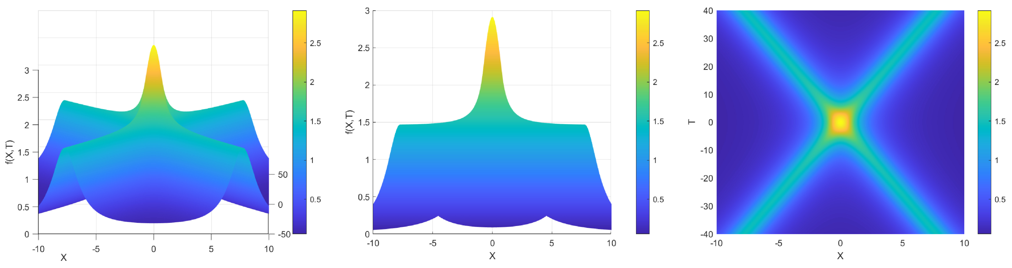
When $n=5$, the interaction between the two solitons can be expressed as

$$\begin{array}{c}\hfill F=\frac{2m_1^3}{1+m_1^6{\left[X-\frac{1}{2}{\left(m_1^3\right)}^{3}T-{\delta }_1^3\right]}^2}+\frac{2m_1^3}{1+m_1^6{\left[-X-\frac{1}{2}{\left(m_1^3\right)}^{3}T-{\delta }_1^3\right]}^2}.\end{array}$$

(50)

We plotted the front, side, and top views of the interaction between the two solitons when $m_1=0.9$ (see Figure 2). As shown in Figure 2, owing to the interaction of two symmetrically placed solitary waves, a hump appeared and grew along the x-axis with time; however, it stopped growing after a period of time. This is a typical Mach-reflection phenomenon. Therefore, the hump is referred to as a Mach stem.

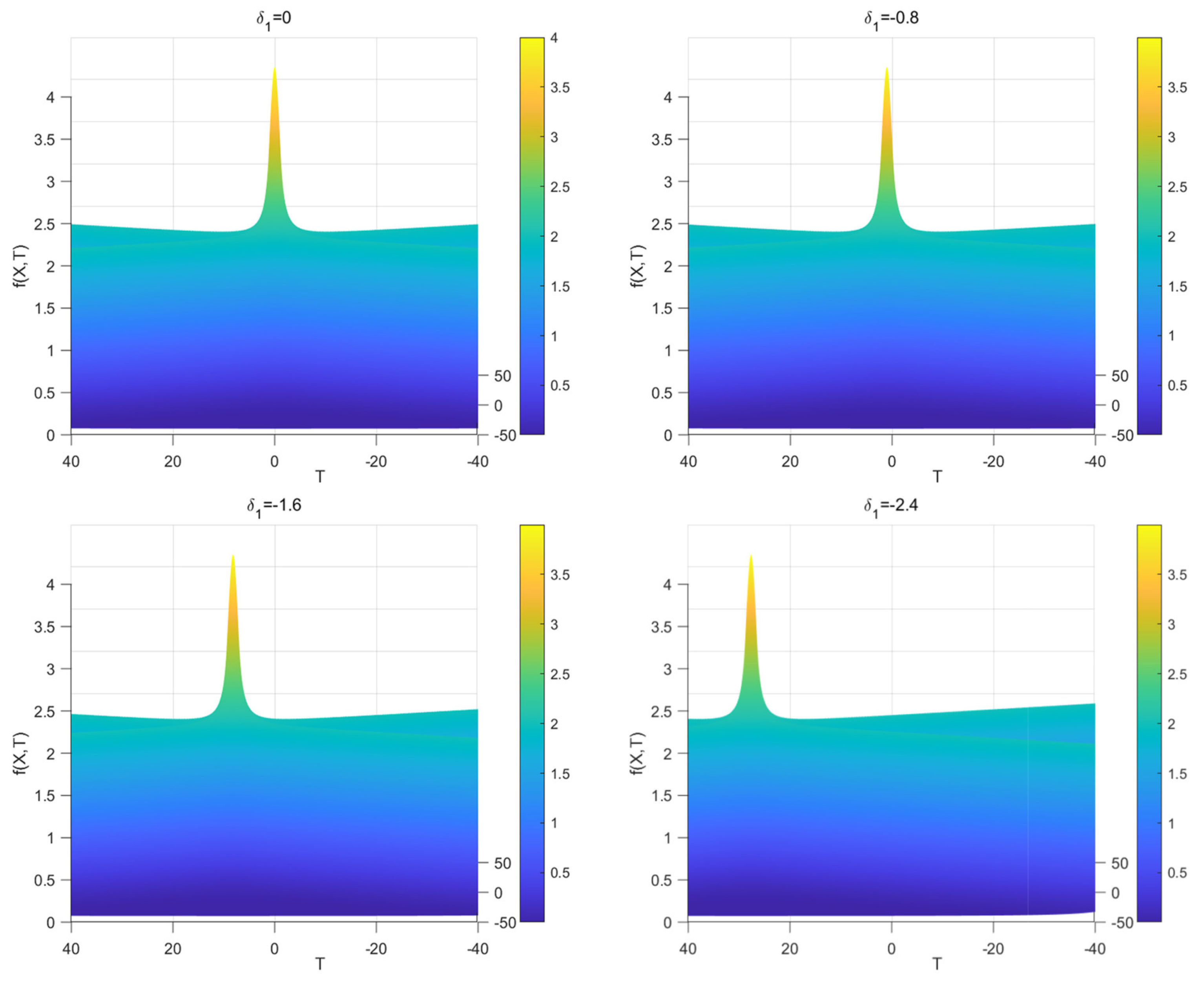
Further, we plot the interaction of the two solitons for different values ${\delta }_1$, as shown in Figure 3. From Figure 3, we can observe that with a decrease in the ${\delta }_1$ value, the shape and size of the Mach stem did not change, but its generation time was gradually delayed. This shows that a change in the ${\delta }_1$ value will not change the shape of the Mach stem, but will have an effect on the time when Mach reflection occurs, and as the ${\delta }_1$ value decreases, the effect becomes increasingly significant.

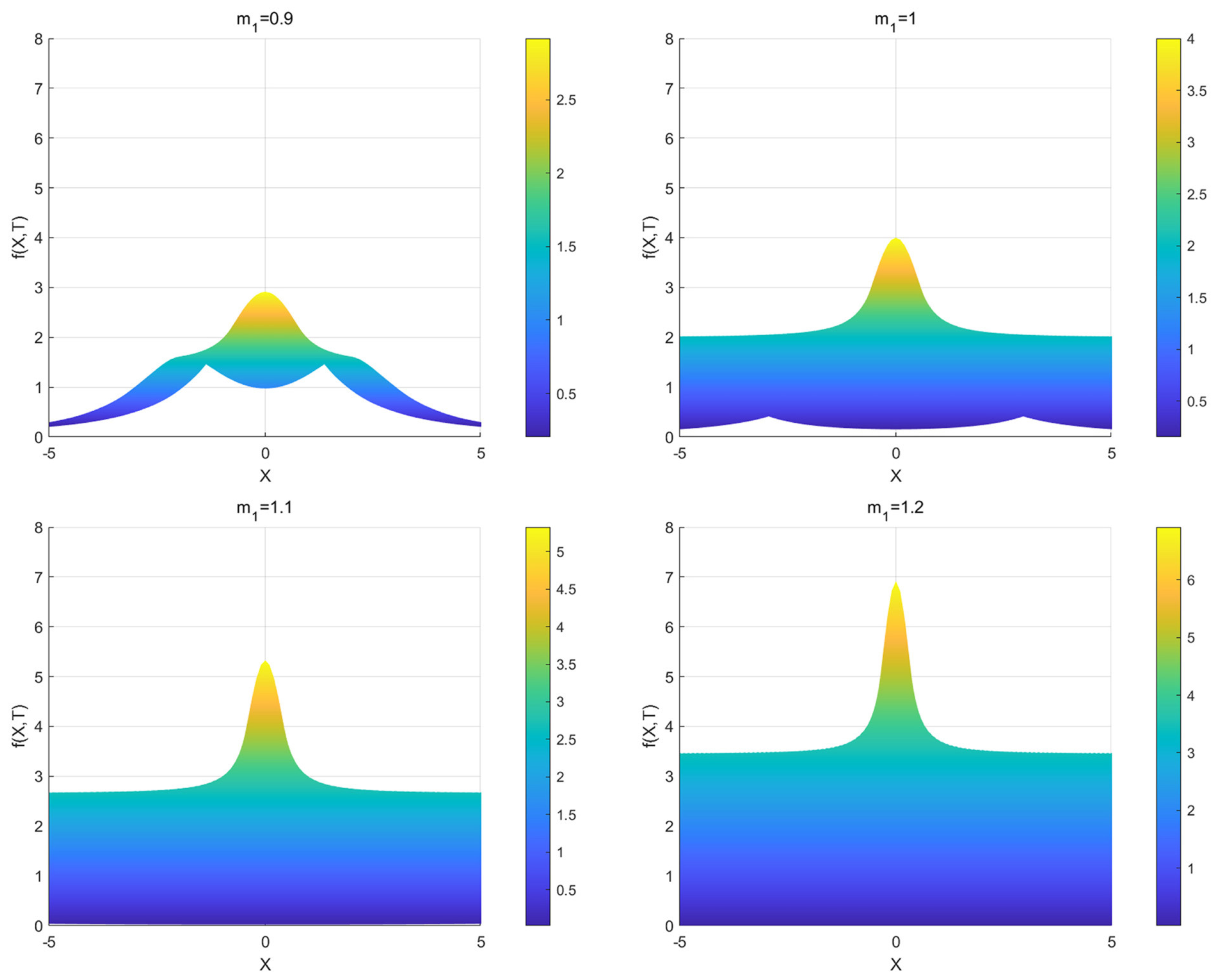
To further study the factors influencing the Mach stem, we drew soliton interaction diagrams for different $m_1$ values, as shown in Figure 4.

As shown in Figure 4, with an increase in $m_1$, the amplitude of the Mach stem gradually increases, but the wave width gradually decreases.

5. Conclusions

Using a multiscale analysis and perturbation method, the Benjamin–Ono equation with variable coefficients describing the propagation of internal solitary waves in the ocean is derived. To better describe the propagation characteristics of solitary waves, we derived a higher-order variable-coefficient integral differential (Benjamin–Ono) equation. Furthermore, based on Hirota’s bilinear method, we obtain the bilinear form and multi-soliton solution of the model. Then, we studied the interaction of the soliton, which led to the discovery of the Mach reflection. The results showed that ${\delta }_1$ only affected the production time of the Mach stem; however, it did not affect its shape. $m_1$ affects the shape of the Mach stem; with an increase in $m_1$, the amplitude of the Mach stem gradually increases, but the wave width gradually decreases.

References

- Chen, J.; Feng, B.; Chen, Y. Bilinear Bäcklund transformation, Lax pair, and multi-soliton solution for a vector Ramani equation. Mod. Phys. Lett. B 2017, 12, 1750133. [Google Scholar] [CrossRef]
- Magalhaes, J.M.; da Silva, J.C.; Nolasco, R.; Dubert, J.; Oliveira, P.B. Short timescale variability in large-amplitude internal waves on the western Portuguese shelf. Cont. Shelf Res. 2022, 246, 104812. [Google Scholar] [CrossRef]
- Endoh, T.; Tsutsumi, E.; Hong, C.-S.; Baek, G.-N.; Chang, M.-H.; Yang, Y.J.; Matsuno, T.; Lee, J.H. Estimating propagation speed and direction, and vertical displacement of second-mode nonlinear internal waves from ADCP measurements. Cont. Shelf Res. 2022, 233, 104644. [Google Scholar] [CrossRef]
- Zou, P.X.; Bricker, J.D.; Uijttewaal, W.S. The impacts of internal solitary waves on a submerged floating tunnel. Ocean Eng. 2021, 238, 109762. [Google Scholar] [CrossRef]
- Song, Z.J.; Teng, B.; Gou, Y.; Lu, L.; Shi, Z.M.; Xiao, Y.; Qu, Y. Comparisons of internal solitary wave and surface wave actions on marine structures and their responses. Appl. Ocean Res. 2011, 33, 120–129. [Google Scholar] [CrossRef]
- Yu, D.; Zhang, Z.G.; Dong, H.; Yang, H. A novel dynamic model and the oblique interaction for ocean internal solitary waves. Nonlinear Dyn. Commun. Nonlinear Sci. Numer. Simul. 2021, 95, 105622. [Google Scholar] [CrossRef]
- He, M.; Khayyer, A.; Gao, X.; Xu, W.; Liu, B. Theoretical method for generating solitary waves using plungertype wavemakers and its Smoothed Particle Hydrodynamics validation. Appl. Ocean Res. 2021, 106, 102414. [Google Scholar] [CrossRef]
- Cai, S.Q.; Long, X.M.; Dong, D.P.; Wang, S.G. Background current affects the internal wave structure of the northern South China Sea. Prog. Nat. Sci. 2008, 18, 585–589. [Google Scholar] [CrossRef]
- He, Y.; Gao, Z.; Luo, J.; Luo, S.; Liu, X. Characteristics of internal-wave and internal-tide deposits and their hydrocarbon potential. Pet. Sci. 2008, 5, 37–44. [Google Scholar] [CrossRef]
- Farmer, D.; Li, Q.; Park, J.H. Internal wave observations in the South China Sea: The role of rotation and non-linearity. Atmos. Ocean 2009, 47, 267–280. [Google Scholar] [CrossRef]
- Zhang, Y.; Deng, B.; Zhang, M. Analysis of the relation between ocean internal wave parameters and ocean surface fluctuation. Front. Earth Sci. 2019, 13, 336–350. [Google Scholar] [CrossRef]
- Kudryavtsev, V.N. Interaction between the surface and internal waves: The modulation and maser mechanisms. Phys. Oceanogr. 1993, 4, 357–375. [Google Scholar] [CrossRef]
- Bourgault, D.; Galbraith, P.; Chavanne, C. Generation of internal solitary waves by frontally forced intrusions in geophysical flows. Nat. Commun. 2016, 7, 13606. [Google Scholar] [CrossRef]
- Guo, C.; Chen, X. A review of internal solitary wave dynamics in the northern South China Sea. Prog. Oceanogr. 2014, 121, 7–23. [Google Scholar] [CrossRef]
- Geng, M.H.; Song, H.B.; Guan, Y.X.; Bai, Y. Analyzing amplitudes of internal solitary waves in the northern South China Sea by use of seismic oceanography data. Deep Sea Res. Part I Oceanogr. Res. Pap. 2019, 146, 1–10. [Google Scholar] [CrossRef]
- Zhang, X.D.; Li, X.F.; Zhang, T. Characteristics and generations of internal wave in the Sulu Sea inferred from optical satellite images. J. Oceanol. Limnol. 2020, 38, 1435–1444. [Google Scholar] [CrossRef]
- Tensubam, C.M.; Raju, N.J.; Dash, M.K.; Barskar, H. Estimation of internal solitary wave propagation speed in the Andaman Sea using multi-satellite images. Remote Sens. Environ. 2021, 252, 112123. [Google Scholar] [CrossRef]
- Zhi, C.H.; Chen, K.; You, Y.X. Internal solitary wave transformation over the slope: Asymptotic theory and numerical simulation. J. Ocean Eng. Sci. 2018, 3, 83–90. [Google Scholar] [CrossRef]
- Zhang, R.; Yang, L.; Liu, Q.; Yin, X. Dynamics of nonlinear Rossby waves in zonally varying ow with spatial-temporal varying topography. Appl. Math. Comput. 2019, 346, 666–679. [Google Scholar]
- Huang, X.D.; Huang, S.W.; Zhao, W.; Zhang, Z.W.; Zhou, C.; Tian, J.W. Temporal variability of internal solitary waves in the northern South China Sea revealed by long-term mooring observations. Prog. Oceanogr. 2022, 201, 102716. [Google Scholar] [CrossRef]
- Helfrich, K.R.; Ostrovsky, L. Effects of rotation and topography on internal solitary waves governed by the rotating Gardner equation. Nonlinear Process. Geophys. Discuss. 2022, 29, 207–218. [Google Scholar] [CrossRef]
- Weinstein, M.I. Lyapunov stability of ground states of nonlinear dispersive evolution equations. Commun. Pure Appl. Math. 1986, 39, 51–67. [Google Scholar] [CrossRef]
- Chen, L.G.; Yang, L.G.; Zhang, R.G.; Cui, J.F. Generalized (2 + 1)-dimensional mKdV-Burgers equation and its solution by modified hyperbolic function expansion method. Results Phys. 2019, 13, 102280. [Google Scholar] [CrossRef]
- Mirie, R.M.; Su, C.H. Internal solitary waves and their head-on collision. Part 1. J. Fluid Mech. 1984, 147, 213–231. [Google Scholar] [CrossRef]
- Keulegan, G.H. Characteristics of internal solitary waves. J. Res. Natl. Bur. Stand. 1953, 51, 133–140. [Google Scholar] [CrossRef]
- Long, R.R. Solitary waves in the one- and two-fluid systems. Tellus 1956, 8, 460–471. [Google Scholar] [CrossRef]
- Benjamin, T. Internal waves of finite amplitude and permanent form. J. Fluid Mech. 1966, 25, 241–270. [Google Scholar] [CrossRef]
- Benjamin, T. Internal waves of permanent form in fluids of great depth. J. Fluid Mech. 1967, 29, 559–592. [Google Scholar] [CrossRef]
- Benney, D.J. Long non-linear waves in fluid flows. J. Math. Phys. 1966, 45, 52–63. [Google Scholar] [CrossRef]
- Ono, H. Algebraic Solitary Waves in Stratified Fluids. J. Phys. Soc. Jpn. 1975, 39, 1082–1091. [Google Scholar] [CrossRef]
- Chen, Y.N.; Wang, K.J. On the Wave Structures to the (3 + 1)-Dimensional Boiti-Leon-Manna-Pempinelli Equation in Incompressible Fluid. Axioms 2023, 12, 519. [Google Scholar] [CrossRef]
- Boyd, J.P.; Xu, Z.J. Numerical and perturbative computations of solitary waves of the Benjamin-Ono equation with higher order nonlinearity using Christovrational basis functions. J. Comput. Phys. 2012, 231, 1216–1229. [Google Scholar] [CrossRef]
- Adem, A.; Khalique, C. Exact Solutions and Conservation Laws of a Two-Dimensional Integrable Generalization of the Kaup-Kupershmidt Equation. J. Appl. Math. 2013, 2013, 647313. [Google Scholar] [CrossRef]
- Yang, D.N. N-soliton, breather, M-lump and interaction dynamics for a (2 + 1)-dimensional KdV equation with variable coefficients. Results Phys. 2023, 46, 106324. [Google Scholar] [CrossRef]
- Zhang, Y.; Dong, H.H.; Fang, Y. Rational and Semi-Rational Solutions to the (2 + 1)-Dimensional Maccari System. Axioms 2022, 11, 472. [Google Scholar] [CrossRef]
- Grimshaw, R.; Pelinovsky, E.; Poloukhina, O. Higher-order Korteweg-de Vries models for internal solitary waves in a stratified shear flow with a free surface. Nonlinear Process. Geophys. 2002, 9, 221–235. [Google Scholar] [CrossRef]
- Kaya, D.; El-Sayed, S.M. On a generalized fifth order KdV equations. Phys. Lett. A 2003, 310, 44–51. [Google Scholar] [CrossRef]
- Duffy, B.R.; Parkes, E.J. Travelling solitary wave solutions to a seventh-order generalized KdV equation. Phys. Lett. A 1996, 214, 271–272. [Google Scholar] [CrossRef]
- Craig, W.; Guyenne, P.; Kalisch, H. Hamiltonian long wave expansions for free surfaces and interfaces. Commun. Pure Appl. Math. 2005, 58, 1587–1641. [Google Scholar] [CrossRef]
- Germán, F.; Felipe, L. Benjamin Ono Equation with Unbounded Data. J. Math. Anal. Appl. 2000, 247, 426–447. [Google Scholar]
- Tsuji, H.; Oikawa, M. Oblique interaction of internal solitary waves in a two-layer fluid of infinite depth. Fluid Dyn. Res. 2001, 29, 251–267. [Google Scholar] [CrossRef]
- Russell, J.S. Report on Waves: Made to the Meetings of the British Association in 1842–43; Creative Media Partners, LLC: London, UK, 1845. [Google Scholar]
- Mach, E.; Wosyka, J. Über einige mechanische Wirkungen des electrischen Funkens. Sitzungsber. Akad. Wiss. Wien 1875, 72, 44–52. [Google Scholar]
- Krehl, P.; van der Geest, M. The discovery of the Mach reflexion effect and its demonstration in an auditorium. Shock Waves 1991, 1, 3–15. [Google Scholar] [CrossRef]
- Ghanbari, B. Employing Hirota’s bilinear form to find novel lump waves solutions to an important nonlinear model in fluid mechanics. Results Phys. 2021, 29, 104689. [Google Scholar] [CrossRef]
- Ye, F.; Tian, J.; Zhang, X.; Jiang, C.; Ouyang, T.; Gu, Y. All Traveling Wave Exact Solutions of the Kawahara Equation Using the Complex Method. Axioms 2022, 11, 330. [Google Scholar] [CrossRef]
- Matsuno, Y. Exact multi-soliton solution of the Benjamin-Ono equation. J. Phys. A Math. Gen. 1979, 12, 619. [Google Scholar] [CrossRef]
- Tsuji, H.; Oikawa, M. Two-dimensional interaction of solitary waves in a modiied Kadomtsev-Petviashvili equation. J. Phys. Soc. Jpn. 2004, 73, 3034–3043. [Google Scholar] [CrossRef]
- Yu, D.; Zhang, Z.G.; Yang, H.W. A new nonlinear integral-differential equation describing Rossby waves and its related properties. Phys. Lett. A 2022, 443, 128205. [Google Scholar] [CrossRef]
Figure 1.
Variation of density with depth z.
Figure 2.
Front, side, and top views of the solution to Equation (50) with , .
Figure 3.
The interaction of the two solitons at different values .
Figure 4.
Interaction of the two solitons at different values .
Disclaimer/Publisher’s Note: The statements, opinions and data contained in all publications are solely those of the individual author(s) and contributor(s) and not of MDPI and/or the editor(s). MDPI and/or the editor(s) disclaim responsibility for any injury to people or property resulting from any ideas, methods, instructions or products referred to in the content. |
© 2023 by the authors. Licensee MDPI, Basel, Switzerland. This article is an open access article distributed under the terms and conditions of the Creative Commons Attribution (CC BY) license (https://creativecommons.org/licenses/by/4.0/).
Share and Cite
MDPI and ACS Style
Ren, Y.; Dong, H.; Zhao, B.; Fu, L. Higher-Order Benjamin–Ono Model for Ocean Internal Solitary Waves and Its Related Properties. Axioms 2023, 12, 969. https://doi.org/10.3390/axioms12100969
AMA Style
Ren Y, Dong H, Zhao B, Fu L. Higher-Order Benjamin–Ono Model for Ocean Internal Solitary Waves and Its Related Properties. Axioms. 2023; 12(10):969. https://doi.org/10.3390/axioms12100969
Chicago/Turabian StyleRen, Yanwei, Huanhe Dong, Baojun Zhao, and Lei Fu. 2023. "Higher-Order Benjamin–Ono Model for Ocean Internal Solitary Waves and Its Related Properties" Axioms 12, no. 10: 969. https://doi.org/10.3390/axioms12100969
Note that from the first issue of 2016, this journal uses article numbers instead of page numbers. See further details here.