
Quadratic Phase Multiresolution Analysis and the Construction of Orthonormal Wavelets in L2(ℝ)


1
Department of Mathematics, IIT Patna, Patna 801106, Bihar, India
2
Department of Mathematics, Texas A&M University-Kingsville, Kingsville, TX 78363-8202, USA
*
Author to whom correspondence should be addressed.
†
These authors contributed equally to this work.
Axioms 2023, 12(10), 927; https://doi.org/10.3390/axioms12100927
Submission received: 2 September 2023
/
Revised: 23 September 2023
/
Accepted: 25 September 2023
/
Published: 28 September 2023
(This article belongs to the Special Issue Differential Equations and Dynamical Systems—Theory and Applications)
Abstract
:The multi-resolution analysis (MRA) associated with quadratic phase Fourier transform (QPFT) serves as a tool to construct orthogonal bases of the . Consequently, it assumes a pivotal role in facilitating potential applications of QPFT. Inspired by the sampling theorem applicable to band-limited signals in the QPFT domain, this paper formulates the development of the MRA linked with QPFT. Subsequently, we develop a method for constructing orthogonal bases for , followed by some examples.
Keywords:
Fourier transform; quadratic phase Fourier transform; Shannon’s sampling theorem; multiresolution analysis; quadratic phase wavelet transform; orthonormal basisMSC:
42C40; 46E30; 42A38; 44A05; 94A121. Introduction
The Fourier transform (FT) is a remarkable discovery in the field of mathematical sciences, which has had a profound impact on many branches of science and engineering [1,2]. Over time, the domain of Fourier analysis has witnessed numerous mathematical breakthroughs, leading to significant advancements and profound implications of the classical Fourier transform. Notable developments that stem from the conventional Fourier transform include the fractional Fourier transform [3,4], linear canonical transform [5], special affine Fourier transform [6], and the relatively recent quadratic-phase Fourier transform [7]. The quadratic-phase Fourier transform (QPFT) extends the classical Fourier transform, incorporating quadratic phase factors into its kernel. In the QPFT, the signal’s time-domain representation is multiplied by a quadratic phase term before computing its frequency-domain representation. This additional quadratic phase term allows for a more flexible analysis of signals with time-varying frequency content. The QPFT provides a unified framework for handling transient and non-transient signals, making it particularly useful for analyzing signals with time-varying properties. It has found applications in various fields, including signal processing, time-frequency analysis, and communication systems. The mathematical expression for the QPFT involves five real parameters that control characteristics of the quadratic phase term. Adjusting these parameters can tailor the QPFT to suit specific signal processing requirements. Overall, the quadratic-phase Fourier transform enhances the traditional Fourier transform’s capabilities, enabling a more versatile and powerful analysis of signals in the time-frequency domain. Shah et al. studied short-time quadratic-phase Fourier transform as well as quadratic-phase wavelet transform (QPWT) with many applications in [8,9]. Also, the quadratic phase Fourier wavelet transform was explored by Prasad and Sharma in [10]. Over the past decades, various integral transforms, including the Fourier, fractional Fourier, and linear canonical transforms, have been extensively explored in time-frequency analysis.
On the other hand, multiresolution analysis (MRA) is a powerful mathematical framework used in signal and image processing introduced by Mallat [11], particularly in the field of wavelet analysis. It provides a systematic and hierarchical approach to analyzing signals or images at different levels of detail or resolution. The concept of MRA is rooted in the idea of representing a signal or an image in terms of a series of subspaces, each capturing different levels of frequency or scale information. Madych [12] established elementary properties of MRA in with scaling functions represented as characteristic functions. Subsequently, Zhang [13] explored scaling functions and wavelets in standard MRA, providing a characterization of the support of the Fourier transform of these scaling functions. Malhotra and Vashisht [14] contributed to understanding scaling functions on Euclidean spaces. The MRA associated with FrWT was also introduced in [15], where FrWT analyzes signals in the time-frequency-FrFD domain. Ahmad [16] studied fractional MRA and associated scaling functions in Dai et al. [17] proposed a novel fractional wavelet transform (FRWT) and studied MRA associated with the developed FRWT, together with the construction of the orthogonal fractional wavelets. Shah and Lone [18,19] studied special affine MRA and the construction of orthonormal wavelets in and studied Shannon’s sampling theorem for the quadratic-phase Fourier transform, which serves as a comprehensive sampling theorem applicable to a broad range of integral transforms. Shah and Tantary [20] formulated the sampling theorem for the QPFT and developed a novel convolution structure for efficient filtering in the quadratic-phase Fourier domain and also gave the advantages of the proposed convolution structure and its integration with the Wigner distribution to filter out undesired signal components. As a generalization of FT, QPFT can represent adaptively signals in both time and FT domains. Therefore, QPFT not only breaks through the limitation of FT in time-Fourier domain analysis but also overcomes the limitation of FT in indicating the signal’s characteristics. QPFT successfully inherits the advantages of MRA for FT. The MRA and the construction of orthogonal wavelets associated with QPFT are crucial in its perspective applications. Thus, detecting the MRA and the construction of the orthogonal wavelets related to QPFT is necessary. Therefore, our primary concern is introducing the notion of quadratic phase MRA, which allows a smoother construction of orthonormal bases simply and insightfully.
The main contributions of this article are as follows:
- To give an alternative proof of Shannon’s sampling theorem associated with the quadratic phase Fourier transform.
- Inspired by the sampling theorem of band-limited signals in the QPFT domain, the MRA associated with quadratic phase wavelet transform is developed.
- Discuss the construction of the orthonormal basis of starting from a given scaling function.
- To give examples of quadratic phase wavelets from given scaling functions.
The rest of the article follows this structure: in Section 2, we offer a comprehensive introduction to the basics, covering the QPFT and also obtain some of its fundamental properties that are new in the literature. Moving on to Section 3, we give an alternative proof of the sampling theorem for the band-limited theorem in the QPFT domain. Based on this sampling theorem, we define a novel MRA and discuss constructing an orthonormal basis for , followed by some examples in Section 4. Finally, in Section 5, we conclude our paper.
2. Preliminaries
In time-frequency analysis, a recent signal processing tool that has garnered attention is the quadratic-phase Fourier transform (QPFT), introduced by Castro et al. [21]. This transformative tool offers a unified approach to handling transient and non-transient signals.
Definition 1.
Given a parameter set , the QPFT of is denoted as and is defined by
where is a quadratic-phase kernel and is given by
and the corresponding inversion formula and Parseval’s formula for the QPFT reads
and
where
Some Properties Associated with the Quadratic Phase Fourier Transform
The lemma below gives some formula for the QPFT, that will be used later in this paper.
Lemma 1.
Let , then the following holds:
- (1)
- (2)
Proof.
Using the definition of the quadratic phase Fourier transform, we have
i.e.,
Now,
If we take then
i.e.,
This finishes the proof. □
The following lemma is an important tool in proving the Shannon’s sampling theorem in the QPFT domain. It says that if a function f is band-limited in the quadratic phase Fourier transform domain, then there is a function g depending on f such that it is band-limited in the Fourier domain. Note that, from here on, we take the value B in as positive.
Lemma 2.
Assume a signal is band limited to in quadratic phase Fourier domain with parameter and Let
then is a signal band-limited in in the Fourier domain.
Proof.
Given,
Taking the Fourier transform, we have
Since is band-limited to so , i.e.,
i.e., supp Thus, Therefore, is band-limited to in the Fourier domain. □
3. Sampling Theorem for Band Limited Signal in QPFT Domain
The sampling theorem, also known as the Nyquist–Shannon sampling theorem, is a fundamental principle in signal processing and digital signal theory. It provides guidance on how to accurately reconstruct a continuous-time analog signal from its discrete samples. The theorem states that, to avoid aliasing and to perfectly reconstruct the original signal, the sampling rate (i.e., the number of samples taken per second) must be at least twice the highest frequency in the analog signal. Mathematically, if a band-limited signal contains a range of k frequencies, it can be accurately reconstructed by taking evenly spaced samples. Taking additional samples would prove redundant, whereas fewer samples would lead to a loss in signal quality. The sampling theorem can be expressed as follows: If a continuous-time signal is band-limited, meaning it contains no frequencies higher than a certain maximum frequency (known as the Nyquist frequency), then the signal can be completely reconstructed from its samples if the sampling rate is greater than or equal to twice the Nyquist frequency.
Inspired by the sampling theorem of band-limited signal in QPFT domain, in this section, the MRA associated with QPFT is established in the next section. The sampling theorem of a band-limited signal associated with QPFT is given by the following theorem.
Theorem 1.
Let signal be band-limited to in QPFT-domain having parameter Then, the following sampling theorem expansion for holds:
where T is the sampling period and satisfies and is called as the Nyquist rate of sampling theorem associated with the quadratic phase Fourier transform.
Proof.
We have
Since is band-limited to in the Fourier domain, by applying the classical Shannon’s sampling theorem, we get
where is the sample period. Therefore,
i.e.,
This finishes the proof. □
4. Multiresolution Analysis Associated with QPFT
This section is devoted to the MRA associated with the QPFT. To introduce the definition, we first start with the following discussion, which has mainly to do with the Shannon’s sampling theorem discussed before. It motivated us to define an MRA associated with the QPFT. In what follows, the results also show the existence of the so-developed MRA.
When the set of band-limited signals in QPFT domain is denoted by i.e.,
where sampling period Therefore, from the sampling theorem, for all we get
Since we have
i.e.,
where
Combining with the orthogonality of we can further obtain that forms an orthonormal basis of
When the set of band-limited signal in the QPFT domain is denoted by i.e.,
It can be further obtained that forms an orthonormal basis of For Equation (1) can be written as
This implies that if and only if This is because
i.e.,
Generally, let
Now, we have
where Thus, forms an orthonormal basis of
Thus, we have
- (a)
- (b)
- (c)
- and
To put it briefly, the sampling theorem for band-limited signals in the QPFT domain serves as the inspiration to establish an orthonormal MRA associated with QPFT.
In this section, our focus lies on introducing the concept of a quadratic phase MRA within the space . This MRA will hold significant importance in developing the quadratic phase orthonormal wavelet basis for . Initially, we present the formal definition of a special affine MRA in .
Definition 2.
An orthogonal MRA associated with QPFT is defined as a sequence of closed subspace such that
- (A)
- (B)
- (C)
- and
- (D)
- There exist a function such that is an orthonormal basis of the subspace where ϕ is called the scaling function of the given MRA.
Lemma 3.
The family , given by the above, constitute an orthonormal system in iff
Proof.
We have
i.e., Now since,
Since forms an orthonormal basis of we have
This implies Set then
Let Then
i.e., is periodic. Therefore,
i.e.,
Conversely, let then
i.e., the system is orthonormal. Hence the conclusion follows. □
Let be an orthonormal MRA of Since and forms an orthonormal basis of so there exists such that
Equation (4) is called the quadratic phase refinement equation. Here,
Now, from Equation (4), we have
Taking QPFT on both sides we get
This gives
Thus,
i.e., where
Equivalently,
where
Since is an orthonormal basis or orthonormal system of so by Lemma 3, we have
Hence, we can write
Observe that
Also,
Hence, from (7)
Now using Equation (6), we have
Given an orthogonal MRA , we define another sequence , of closed subspaces of by . Followed by a definition, these subspace inherit the scaling property of , namely
Moreover, the subspaces are mutually orthogonal with the following decomposition formula
Note that condition (10) means that any orthonormal basis for can be constructed by finding out an orthonormal basis for the subspace . On the other hand, condition (9) implies that the quadratic phase basis can be constructed as long as the orthonormal basis for is found. Therefore, our main concern is to construct a mother function in such that forms an orthonormal basis of .
Suppose , there exists such that
Since and are orthogonal in we have
Observe that
Similarly,
Therefore,
From Equation (17), we conclude that
This implies
Equation (18) can be written in the matrix form as
where denotes the conjugate transpose of M, is the identity matrix, and
Since and cannot vanish together on a set of non-zero measures due to the orthogonal property, there exists a - periodic function such that
Since,
Using Equation (8),
Therefore, we have
Therefore, is - periodic, it can be expressed as
where
Therefore, where
Therefore,
where Now,
Therefore,
Thus, from (20)
In particular, for using (13), we have
This implies
Integrating both sides, we get
Therefore, equivalently, we can write the wavelet coefficients of Equation (11) as
The above discussion can be summarized in the following theorem.
Theorem 2.
If is the quadratic phase MRA associated with the scaling function then there exists a function ψ such that
where is given by (21) with , i.e., the system is an orthonormal basis of
Example 1.
It is observed in the earlier discussion that the function is a scaling function for the quadratic phase MRA where is an orthonormal basis of the subspace Hence,
which results in
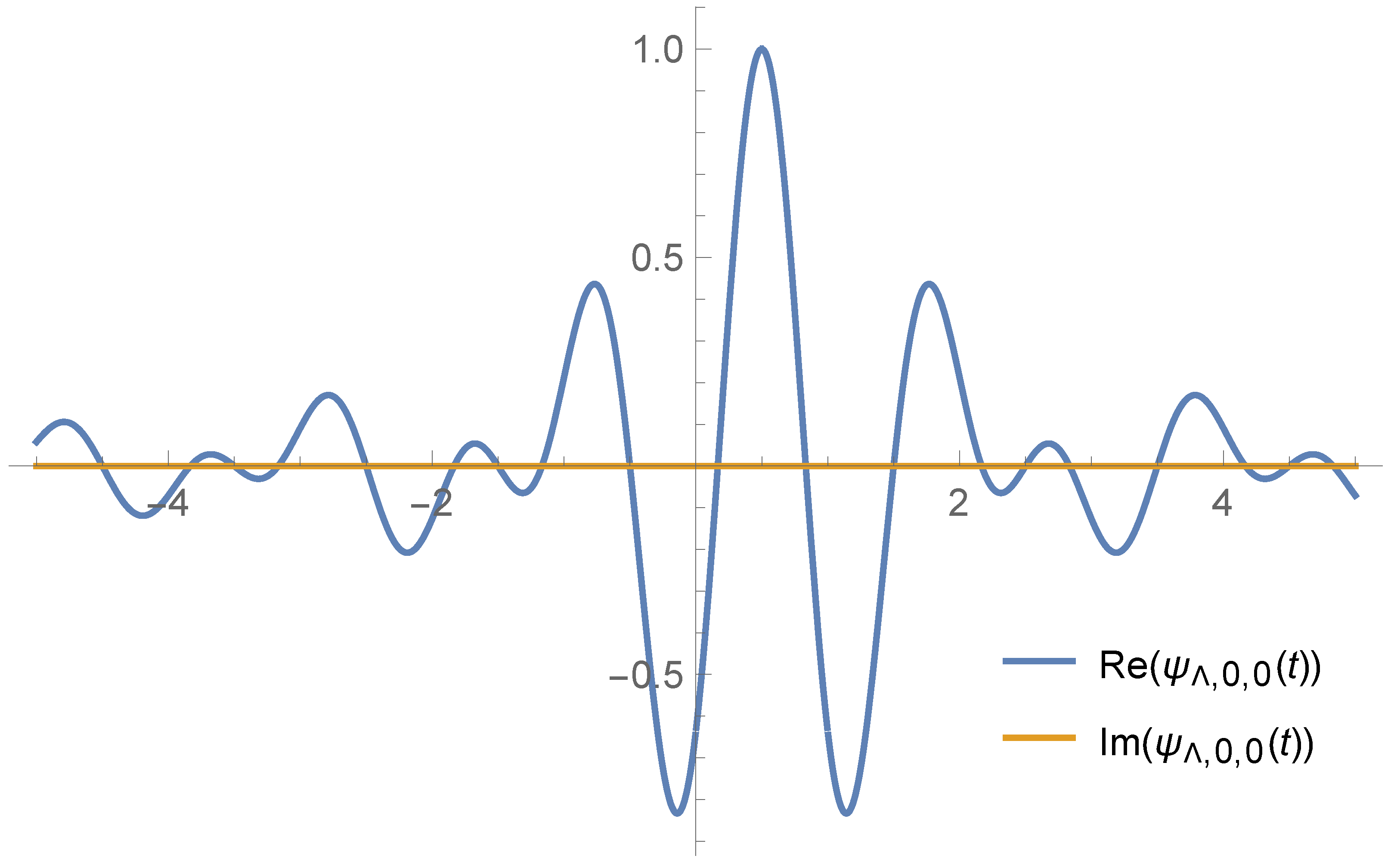
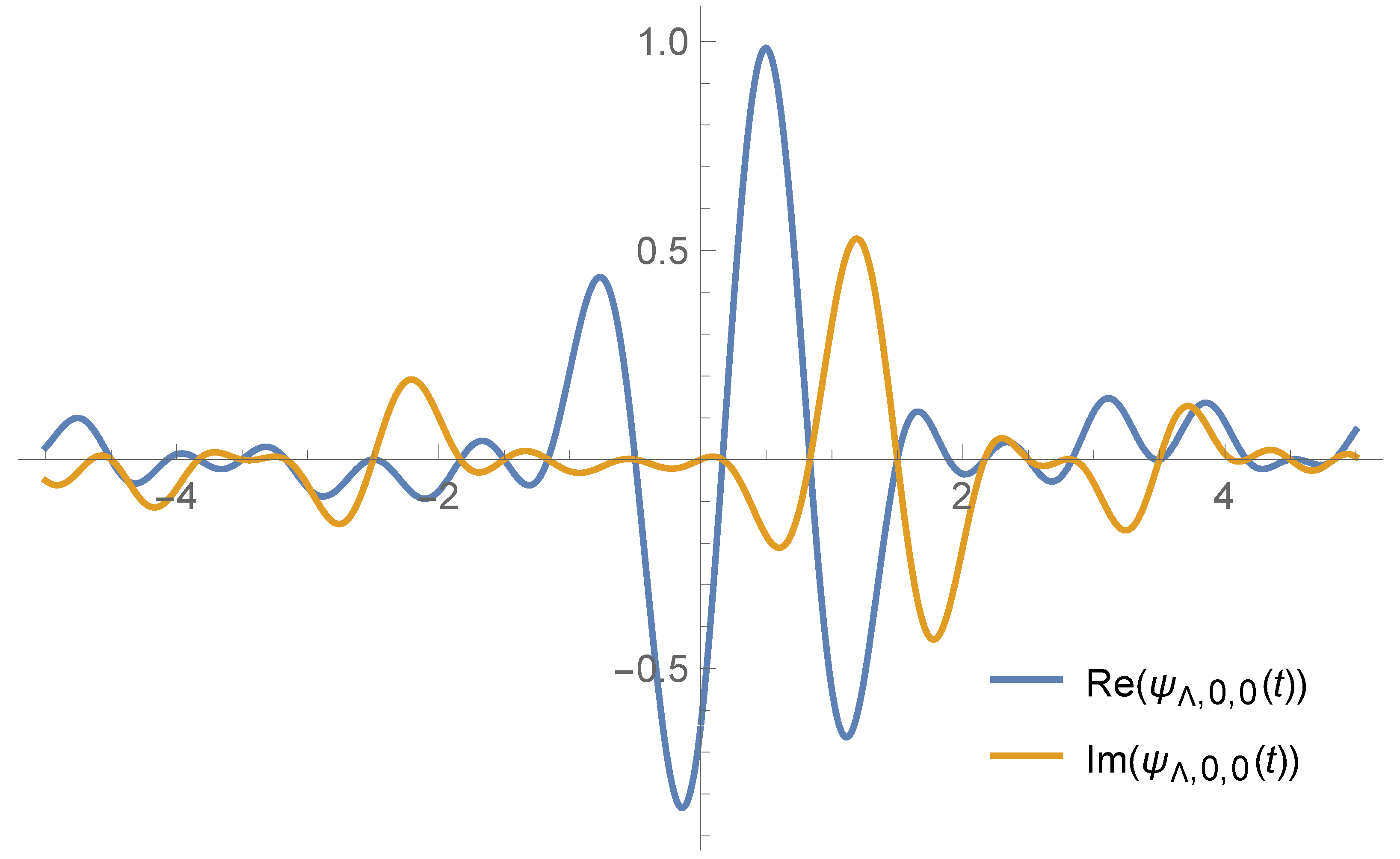
Thus, the quadratic phase wavelet corresponding to the scaling function is given by
The plots of the real and imaginary part of are given below for the particular choice of the parameter and
Example 2.
Let where is a characteristic function on It is a matter of simple verification that the set forms an orthonormal system. Hence it forms an orthonormal basis of the set thus is a scaling function associated with the MRA Thus,
resulting in
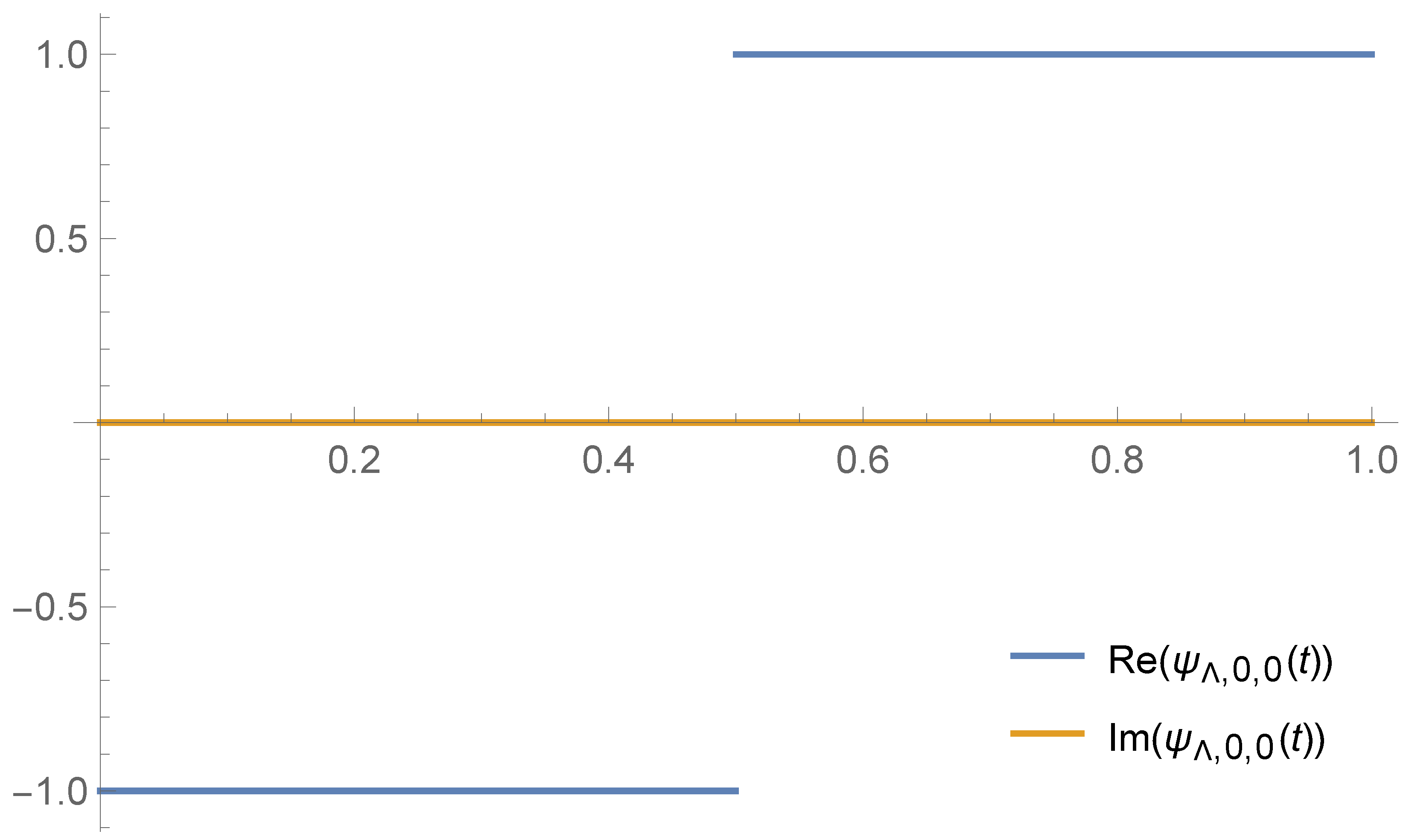
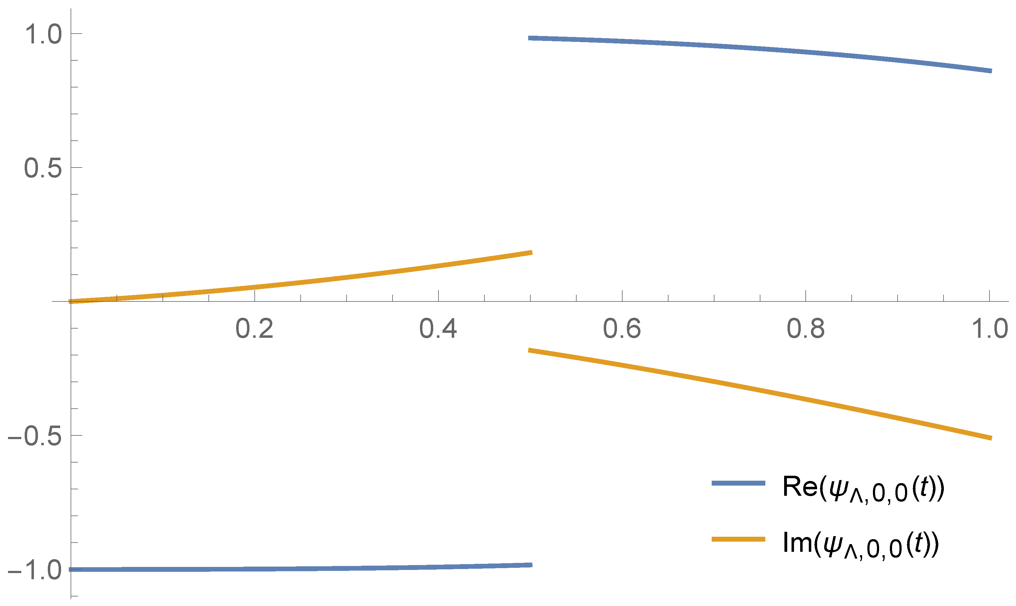
Thus, the quadratic phase wavelet corresponding to the scaling function is given by
The plots of the real and imaginary parts of are given below for the particular choice of the parameter and
Remark 1.
By virtue of Lemma 3 and the Definition 2 of MRA we can say that any function that serves as a scaling function in the classical MRA will also serve as a scaling function for the MRA given by Definition 2. But, depending on the choice of parameters Λ, we can have different quadratic phase wavelets and thus different families of orthonormal bases of . In particular, for the choice of the parameter we get the classical wavelets and the quadratic phase wavelets for (see Figure 1, Figure 2, Figure 3 and Figure 4). The flexibility in the choice of the parameters results in the development of some novel families of orthonormal bases of corresponding to the same scaling function.
5. Conclusions
The MRA and the construction of orthogonal wavelets for QPFT play a vital role in facilitating prospective applications of QPFT. In this paper, we gave an alternative proof of the Shannon’s sampling theorem applicable to the band-limited signal in the QPFT. Inspired by the theorem, we developed an MRA associated with QPFT. Subsequently, we discussed the construction of the quadratic phase wavelets for a given scaling function, followed by some of its examples.
Author Contributions
Conceptualization, B.G. and A.K.V.; methodology, B.G. and N.K.; software, B.G.; validation, B.G., A.K.V. and R.P.A.; formal analysis, B.G. and N.K.; investigation, B.G. and A.K.V.; resources, R.P.A.; writing—original draft preparation, B.G. and N.K.; writing—review and editing, B.G. and N.K.; visualization, A.K.V. and R.P.A.; supervision, A.K.V. and R.P.A.; project administration, A.K.V.; funding acquisition, B.G., A.K.V. and N.K. All authors have read and agreed to the published version of the manuscript.
Funding
This work is partly supported by UGC File No. 16-9 (June 2017)/2018(NET/CSIR), DST SERB FILE NO. MTR/2021/000907 and CSIR File No. 09/1023(0035)/2020-EMR-I), New Delhi, India.
Data Availability Statement
Not applicable.
Conflicts of Interest
The authors declare no conflict of interest.
Abbreviations
The following abbreviations are used in this manuscript:
| MDPI | Multidisciplinary Digital Publishing Institute |
| DOAJ | Directory of open access journals |
| TLA | Three letter acronym |
| LD | Linear dichroism |
References
- Debnath, L.; Shah, F.A. Wavelet Transforms and Their Applications; Birkhäuser: New York, NY, USA, 2015. [Google Scholar]
- Debnath, L.; Shah, F.A. Lecture Notes on Wavelet Transforms; Birkhäuser: Boston, MA, USA, 2017. [Google Scholar]
- Namias, V. The fractional order Fourier transform and its application to quantum mechanics. IMA J. Appl. Math. 1980, 25, 241–265. [Google Scholar] [CrossRef]
- Almeida, L.B. The fractional Fourier transform and time-frequency representations. IEEE Trans. Signal Process. 1994, 42, 3084–3091. [Google Scholar] [CrossRef]
- Xu, T.Z.; Li, B.Z. Linear Canonical Transform and Its Applications; Science Press: Beijing, China, 2013. [Google Scholar]
- Abe, S.; Sheridan, J.T. Generalization of the fractional Fourier transformation to an arbitrary linear lossless transformation an operator approach. J. Phys. Math. Gen. 1994, 27, 4179. [Google Scholar] [CrossRef]
- Castro, L.P.; Haque, M.R.; Murshed, M.M.; Saitoh, S.; Tuan, N.M. Quadratic Fourier transforms. Ann. Funct. Anal. 2014, 5, 10–23. [Google Scholar] [CrossRef]
- Shah, F.A.; Lone, W.Z.; Tantary, A.Y. Short-time quadratic-phase Fourier transform. Optik 2021, 245, 167689. [Google Scholar] [CrossRef]
- Shah, F.A.; Lone, W.Z. Quadratic-phase wavelet transform with applications to generalized differential equations. Math. Methods Appl. Sci. 2022, 45, 1153–1175. [Google Scholar] [CrossRef]
- Prasad, A.; Sharma, P.B. The quadratic-phase Fourier wavelet transform. Math. Methods Appl. Sci. 2020, 43, 1953–1969. [Google Scholar] [CrossRef]
- Mallat, S.G. Multiresolution approximations and wavelet orthonormal bases of L2(ℝ). Trans. Am. Math. Soc. 1989, 315, 69–87. [Google Scholar]
- Madych, W.R. Some elementary properties of multiresolution analyses of L2(ℝn). In Wavelets: A Tutorial in Theory and Applications; Chui, C.K., Ed.; Academic Press: Boston, MA, USA, 1992; pp. 259–277. [Google Scholar]
- Zhang, Z. Supports of Fourier transforms of scaling functions. Appl. Comput. Harmon. Anal. 2007, 22, 141–156. [Google Scholar] [CrossRef]
- Malhotra, H.K.; Vashisht, L.K. On scaling functions of non-uniform multiresolution analysis in L2(ℝ). Int. J. Wavelets Multiresolut. Inf. Process. 2020, 18, 1950055. [Google Scholar] [CrossRef]
- Shi, J.; Liu, X.; Zhang, N. Multiresolution analysis and orthogonal wavelets associated with fractional wavelet transform. Signal Image Video Process. 2015, 9, 211–220. [Google Scholar] [CrossRef]
- Ahmad, O.; Sheikh, N.A.; Shah, F.A. Fractional multiresolution analysis and associated scaling functions in L2(ℝ). Anal. Math. Phys. 2021, 11, 47. [Google Scholar] [CrossRef]
- Dai, H.; Zheng, Z.; Wang, W. A new fractional wavelet transform. Commun. Nonlinear Sci. Numer. Simul. 2017, 44, 19–36. [Google Scholar] [CrossRef]
- Shah, F.A.; Lone, W.Z. Special affine multiresolution analysis and the construction of orthonormal wavelets in L2(ℝ). Appl. Anal. 2023, 102, 2540–2566. [Google Scholar] [CrossRef]
- Lone, W.Z.; Shah, F.A. Shift-invariant spaces and dynamical sampling in quadratic-phase Fourier domains. Optik 2022, 260, 169063. [Google Scholar] [CrossRef]
- Shah, F.A.; Tantary, A.Y. Sampling and multiplicative filtering associated with the quadratic-phase Fourier transform. Signal Image Video Process. 2023, 17, 1745–1752. [Google Scholar] [CrossRef]
- Castro, L.P.; Minh, L.T.; Tuan, N.M. New convolutions for quadratic-phase Fourier integral operators and their applications. Mediterr. J. Math. 2018, 15, 13. [Google Scholar] [CrossRef]
Figure 1.
Plot of the real part and imaginary parts of corresponding to .

Figure 2.
Plot of the real part and imaginary parts of corresponding to .

Figure 3.
Plot of the real part and imaginary parts of corresponding to .

Figure 4.
Plot of the real part and imaginary parts of corresponding to .

Disclaimer/Publisher’s Note: The statements, opinions and data contained in all publications are solely those of the individual author(s) and contributor(s) and not of MDPI and/or the editor(s). MDPI and/or the editor(s) disclaim responsibility for any injury to people or property resulting from any ideas, methods, instructions or products referred to in the content. |
© 2023 by the authors. Licensee MDPI, Basel, Switzerland. This article is an open access article distributed under the terms and conditions of the Creative Commons Attribution (CC BY) license (https://creativecommons.org/licenses/by/4.0/).
Share and Cite
MDPI and ACS Style
Gupta, B.; Kaur, N.; Verma, A.K.; Agarwal, R.P. Quadratic Phase Multiresolution Analysis and the Construction of Orthonormal Wavelets in L2(ℝ). Axioms 2023, 12, 927. https://doi.org/10.3390/axioms12100927
AMA Style
Gupta B, Kaur N, Verma AK, Agarwal RP. Quadratic Phase Multiresolution Analysis and the Construction of Orthonormal Wavelets in L2(ℝ). Axioms. 2023; 12(10):927. https://doi.org/10.3390/axioms12100927
Chicago/Turabian StyleGupta, Bivek, Navneet Kaur, Amit K. Verma, and Ravi P. Agarwal. 2023. "Quadratic Phase Multiresolution Analysis and the Construction of Orthonormal Wavelets in L2(ℝ)" Axioms 12, no. 10: 927. https://doi.org/10.3390/axioms12100927
Note that from the first issue of 2016, this journal uses article numbers instead of page numbers. See further details here.