
Bogdanov–Takens Bifurcation Analysis of a Learning-Process Model
1
College of Mathematics and Data Science, Minjiang University, Fuzhou 350108, China
2
HNU-ASU Joint International Tourism College, Hainan University, Haikou 570228, China
3
School of Economics and Management, Southwest Jiaotong University, Chengdu 610031, China
*
Author to whom correspondence should be addressed.
Axioms 2023, 12(9), 853; https://doi.org/10.3390/axioms12090853
Submission received: 8 June 2023
/
Revised: 17 August 2023
/
Accepted: 29 August 2023
/
Published: 31 August 2023
Abstract
:In this paper, as a complement to the works by Monterio and Notargiacomo, we analyze the dynamical behavior of a learning-process model in a case where the system admits a unique interior degenerate equilibrium. Meanwhile, we acquire the sufficient condition for the cusp of codimension 2 and verify that the system undergoes Bogdanov–Takens bifurcation around the cusp. Finally, we give a numerical simulation to support the theoretical results.
1. Introduction
With the development of human society, educational issues [1,2,3,4,5] are gradually attracting people’s attention and are not ignored. Doubts [6] are a universal phenomena during the process of learning knowledge. The influence and significance of doubt in experience of acquiring knowledge are focused on by many scholars [7,8,9]. As time goes by, there exists a dynamic process of mutual transformation between understanding and doubt. That is, understanding can be transformed into doubt, and doubt can also be transformed into understanding [10]. Therefore, Monterio and Notargiacomo [11] proposed that the learning process as the interplay between understanding and doubt can be studied by formulating and analyzing a dynamical system written in term of differential equations. In order to better study this, the entirety of knowledge is divided into two parts: one part is already understood, and the other is still doubted. The first “understanding–doubt” model was put forward as follows.
U and D describe the level of understanding and doubt with time t during the learning process, respectively. and stand for the minimum background required to learn about a subject and the maximum level of doubt that learner can have about a subject that they did not learn about it, respectively. a and b represent the speed of the learning process. The parameters f and g describe the interaction between and and . At the standing point of physical meaning, the term restricts the dynamics to the right triangle domain given by , and . Authors have studied the stability of the boundary equilibria and provided some numerical simulations to verify the theoretical results.
Liu, Ding and Chen performed deep studies of System (1) in [12]. They gave a complete analysis of the qualitative properties of the interior equilibria and a singular line segment. They also investigated some local bifurcation, including transcritical, pitchfork, and Hopf bifurcation [13,14] on isolated equilibrium, and transcritical bifurcation without parameters on non-isolated equilibrium.
However, dynamical behavior of the learning-process model in a case where the system admits a unique interior equilibrium can be studied further. Meanwhile, bifurcation of a higher codimension, which is the Bogdanov–Takens bifurcation of codimension 2, is worth analyzing since, compared to bifurcation of codimension 1, bifurcation of codimension 2 demonstrates more realistic dynamic behavior between understanding and doubt in the learning process.
Compared to the works by Liu, Ding and Chen in [12] we will give the analysis of Bogdanov–Takens bifurcation [15,16,17] of codimension 2 when System (1) admits a unique interior equilibrium (cusp).
This paper is arranged as follows. We obtain the sufficient conditions for the existence of the cusp [18] of codimension 2 in Section 2. In Section 3, we prove that System (1) undergoes Bogdanov–Takens bifurcation of codimension 2 and the theoretical results are verified by numerical simulation. A brief ends this paper in Section 4.
2. The Existence of the Cusp of Codimension 2
For simplicity, we make a time rescaling , and System (1) becomes
where .
For physical meaning, we only consider the dynamic behavior of System (2) in the closure for all possibilities of .
The equilibria of System (2) are determined by the following equation:
There exists a singular line segment
and three boundary equilibria . The interior equilibria of System (2) are determined by the following equation:
From , we have
Therefore, from and , we consider quadratic function to have double zeros if , which means that System (2) admits a degenerate equilibrium . Furthermore, if and , then we have
Therefore, System (2) admits a degenerate equilibrium .
In order to ensure , and , the parameters f, g and should satisfy , , and .
Additionally, equilibrium should lie on the right triangle domain , so we have . On the other hand, , and we need to ensure , thus holds.
Summing up the above, we have the following theorem:
Theorem 1.
Based on , , and
there exists a unique degenerate equilibrium in system (2).
Combining above results with Theorem 2.1 in [12], we have the following theorem:
Theorem 2.
Depending on condition for existence of equilibrium , boundary equilibria of system (2) have the following qualitative properties:
The origin : is a saddle;
Equilibrium : is a stable node;
Equilibrium : is an unstable node.
In the following, we determine type of equilibrium .
Theorem 3.
From condition for existence of degenerate equilibrium and
equilibrium is a cusp of codimension 2.
Proof.
By Remark 1 of Section 2.13 in [19], we obtain an equivalent system of System (7) in the small neighborhood of as follows
where
If
then , which means that degenerate equilibrium is a cusp of codimension 2. □
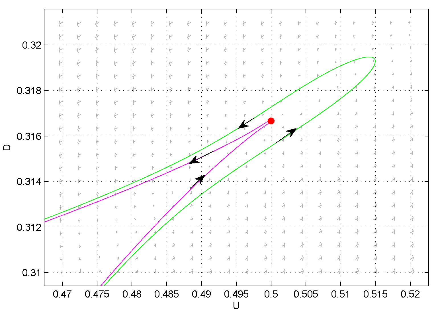
Setting , the phase portrait of cusp of codimension 2 of is described with the help of Matlab; see Figure 1.
Remark 1.
From [11], if doubt destroys comprehension, then and ; if doubt drives comprehension, then and . Therefore, according to sufficient condition for existence of cusp of codimension 2, doubt destroys comprehension.
3. Analysis of Bogdanov–Takens Bifurcation
From Section 2, we know that is a cusp of codimension 2. In this section, we investigate Bogdanov–Takens bifurcation around .
Theorem 4.
Under the condition for the existence of equilibrium , which is a cusp of codimension 2, we choose α and r as bifurcation parameters. As the parameters disturb around , system (2) undergoes Bogdanov–Takens bifurcation in a small neighborhood of .
Proof.
We choose and r as two bifurcation parameters and replace and r with and , respectively, in System (2). Then, we acquire the unfolding system of System (2):
where is a parameter vector in a small neighborhood of origin. Obviously, when , System (9) has a unique positive equilibrium , which is a cusp of codimension 2. For simplicity, the universal unfolding will be obtained with the help of a series of transformation in the following.
Making a translation transformation , equilibrium will be translated into , then System (9) becomes
where
To save space, the current expression consists of a previous expression when System (10) undergoes each approximate identity transformation in the following.
To remove from System (11), introduce a new time variable with and make , then System (11) becomes (rewriting as t):
where
From , when (i = 1, 2) are small, we have . Therefore, can be reduced into with the following coordinates change:
then System (12) can be transformed into (rewriting as t)
where
From , when (i = 1, 2) are small, we have . Employing the change of variables again,
we obtain the universal unfolding of System (9),
where
The transversality condition
holds. Therefore, from the Bogdanov–Takens bifurcation theorem [19,20], System (2) undergoes a Bogdanov–Takens bifurcation of codimension 2, which includes a sequence of bifurcations of codimension 1: saddle-node bifurcation, Hopf bifurcation and homoclinic bifurcation, when the parameters and vary in a small neighborhood of . □
Turning to Matlab, we provide some data groups to simulate the dynamic process of Bogdanov–Takens bifurcation to support the theoretical results. Let and , then and System (9) becomes
System (16) will present different phase portraits according to following six examples for disturbance of and .
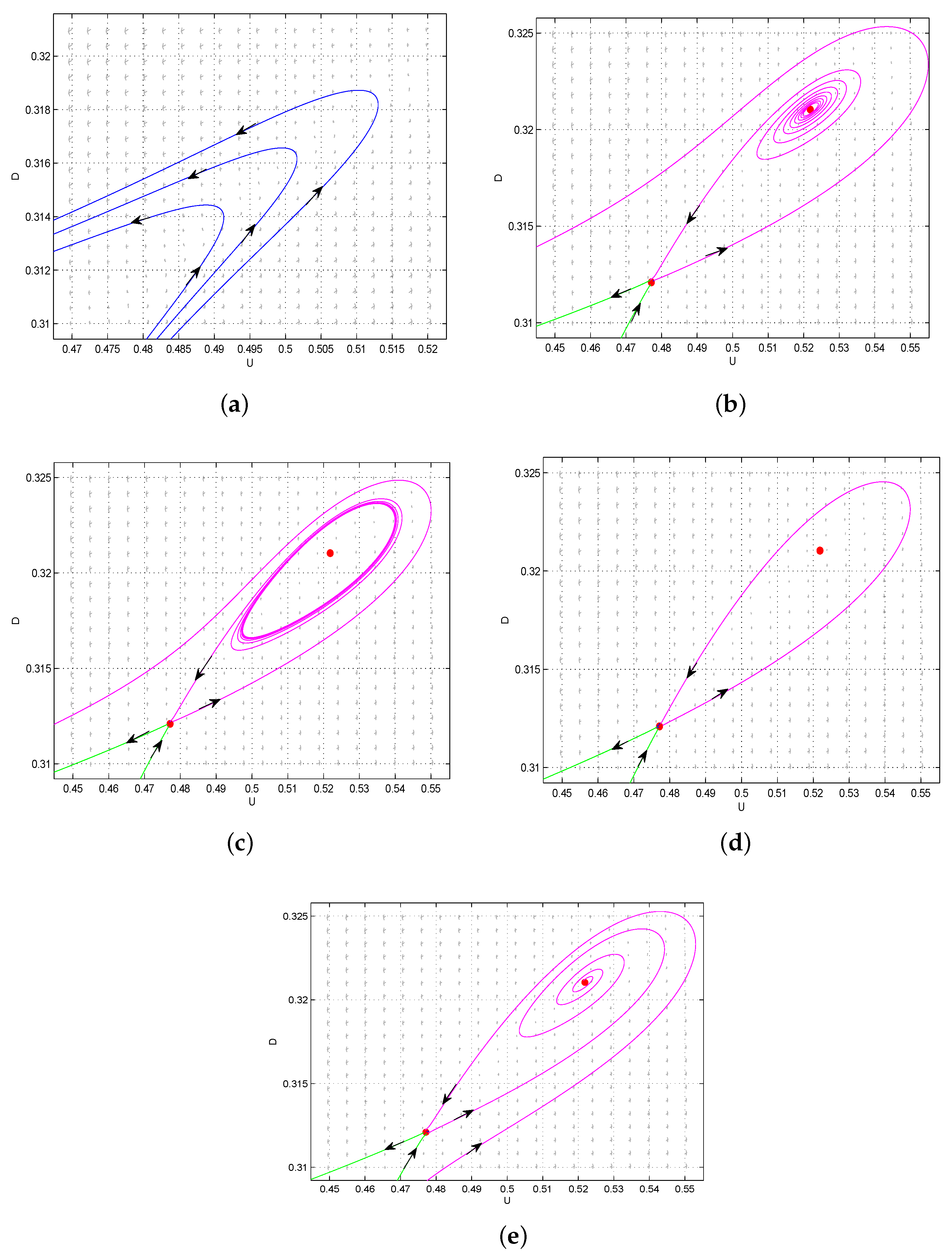
Example 4: take , System (16) has a stable focus surrounded by an unstable limit cycle; see Figure 2c.
4. Conclusions
The dynamical behavior of System (1) around the unique positive equilibrium was investigated in this manuscript. The case that the Jacobian matrix has two zero eigenvalues is focused. We proved that equilibrium is a cusp of codimension 2 through linear transformation and normal form theory [20].
From Theorems 1 and 3, in order to ensure that System (1) admits a cusp of codimension 2, parameters f and g must satisfy and . Therefore, doubt should be regarded as restraining force and destroys comprehension in the learning process if System (1) has a cusp of codimension 2 and undergoes Bogdanov–Takens bifurcation of codimension 2.
By Theorem 4, System (1) undergoes Bogdanov–Takens bifurcation of codimension 2, which leads to potentially dramatic changes in the system, hence bifurcation of codimension 2 should be not ignored. Due to a saddle-node bifurcation, the number of the interior equilibrium is zero, one, or two as parameters and r are disturbed.Thus, there are some values of parameters such as that understanding and doubt co-exist in the form of interior equilibrium for different initial values. Through a Hopf bifurcation, there is a limit cycle appearing in System (1). As seen in Figure 2c, an unstable limit cycle is produced by the Hopf bifurcation. When all initial values lying inside the limit cycle, the orbit will tend to the interior equilibrium at last. That is, understanding and doubt will reach a steady state. In other words, knowledge can not be absorbed fully; once the learner decreases the time to understand, doubts regarding the knowledge will increase. From homoclinic bifurcation, a homoclinic loop appears in System (1). As seen in Figure 2d, an unstable homoclinic loop is consisted of a saddle and an unstable homoclinic orbit, which means that understanding and doubt co-exist in the form of an interior equilibrium for all initial values lying inside the homoclinic loop.
It is noteworthy that when all initial values lying outside the unstable limit cycle and unstable homoclinic loop, combining with Theorem 2, the orbit will tend to the equilibrium . That is, if enough time was taken, the learner will feel confident with the knowledge at last.
Above all, the occurrences of Bogdanov–Takens bifurcation yields to more complex dynamical behavior, including bifurcations of codimension one. It is very sensitive to the choice of coefficient of difficulty in studying material and the speed of the learning process, which indicates that the selection of learning and teaching methods should be put forward higher requirements for students and teachers in education.
However, the existence condition of Bogdanov–Takens of codimension 2 is sufficient and the Bogdanov–Takens bifurcation of higher codimensions in the distribution functions [21] is worth studying in the future.
Author Contributions
Formal analysis, Z.Z.; Writing—review and editing, Y.G., Z.Z. and Y.G. contributed equally to the writing of this paper. All authors have read and agreed to the published version of the manuscript.
Funding
This research was funded by the Natural Science Foundation of Fujian Province grant number 2020J01499.
Data Availability Statement
Not applicable.
Acknowledgments
The authors are thankful to Hebai Chen for their valuable suggestions to upgrade the manuscript significantly.
Conflicts of Interest
The authors declare no conflict of interest.
References
- Monteiro, L.H. Population dynamics in educational institutions considering the student satisfaction. Commun. Nonlinear Sci. Numer. Simul. 2016, 30, 236–242. [Google Scholar] [CrossRef]
- Marton, F.; Säljö, R. On qualitative differences in learning: I-Outcome and process. Br. J. Educ. Psychol. 1976, 46, 4–11. [Google Scholar] [CrossRef]
- Bacdayan, W. A mathematical analysis of the learning production process and a model for determining what matters in education. Econ. Educ. Rev. 1997, 16, 25–37. [Google Scholar] [CrossRef]
- Pritchard, D.E.; Lee, Y.J.; Bao, L. Mathematical learning models that depend on prior knowledge and instructional strategies. Phys. Rev. Spec.-Top.-Phys. Educ. Res. 2008, 4, 010109. [Google Scholar] [CrossRef]
- Bordogna, M.; Albano, E.V. Phase transitions in a model for social learning via the Internet. Int. J. Mod. Phys. 2001, 12, 1241–1250. [Google Scholar] [CrossRef]
- Hecht, J.M. Doubt: A History; Harper Collins: New York, NY, USA, 2004. [Google Scholar]
- Schechter, C.; Ganon-Shilon, S. Reforming schools: The collective doubting perspective. Int. J. Educ. Manag. 2015, 29, 62–72. [Google Scholar] [CrossRef]
- Mills, C.M. Knowing when to doubt: Developing a critical stance when learning from others. Dev. Psychol. 2013, 49, 404–418. [Google Scholar] [CrossRef] [PubMed]
- Srikantia, P.; Pasmore, W. Conviction and doubt in organizational learning. J. Organ. Chang. Manag. 1996, 9, 42–53. [Google Scholar] [CrossRef]
- Burbules, N.C. Aporias, webs, and passages: Doubt as an opportunity to learn. Curric. Inq. 2000, 30, 171–187. [Google Scholar] [CrossRef]
- Monteiro, L.H.; Notargiacomo, P.C.S. Learning process as an interplay between understanding and doubt: A dynamical systems approach. Commun. Nonlinear Sci. Numer. Simul. 2017, 47, 416–420. [Google Scholar] [CrossRef]
- Liu, L.L.; Ding, K.W.; Chen, H.B. Dynamical analysis of a Lotka-Volterra Learning-Process Model. J. Appl. Anal. Comput. 2019, 9, 1855–1871. [Google Scholar] [CrossRef] [PubMed]
- Gou, W.; Jin, Z.; Wang, H. Hopf bifurcation for general network-organized reaction-diffusion systems and its application in a multi-patch predator-prey system. J. Differ. Equ. 2023, 346, 64–107. [Google Scholar] [CrossRef]
- Ma, T.; Meng, X.; Hayat, T.; Hobiny, A. Hopf bifurcation induced by time delay and influence of Allee effect in a diffusive predator-prey system with herd behavior and prey chemotaxis. Nonlinear Dyn. 2022, 108, 4581–4598. [Google Scholar] [CrossRef]
- Stróżyna, E.; Żoła̧dek, H. Analytic properties of the complete formal normal form for the Bogdanov-Takens singularity. Nonlinearity 2021, 34, 3046. [Google Scholar] [CrossRef]
- Lu, M.; Xiang, C.; Huang, J.C. Bogdanov-Takens bifurcation in a SIRS epidemic model with a generalized nonmonotone incidence rate. Discret. Contin. Dyn. Syst.-S 2020, 13, 3125–3138. [Google Scholar] [CrossRef]
- Zhu, Z.L.; Chen, Y.M.; Li, Z.; Chen, F.D. Stability and bifurcation in a Leslie-Gower predator-prey model with Allee effect. Int. J. Bifurc. Chaos. 2022, 32, 2250040. [Google Scholar] [CrossRef]
- Xiong, Y.Q.; Han, M.A. Limit cycles appearing from a generalized heteroclinic loop with a cusp and a nilpotent saddle. J. Differ. Equ. 2021, 303, 575–607. [Google Scholar] [CrossRef]
- Perko, L. Differential Equations and Dynamical Systems. In Texts in Applied Mathematics, 3rd ed.; Springer: New York, NY, USA, 2001; Volume 7. [Google Scholar]
- Chow, S.-N.; Li, C.Z.; Wang, D. Normal Forms and Bifurcation of Planar Vector Fields; Cambridge University Press: Cambridge, CA, USA, 1994. [Google Scholar]
- Wang, W.; Cherstvy, A.G.; Liu, X.; Metzler, R. Anomalous diffusion and nonergodicity for heterogeneous diffusion processes with fractional Gaussian noise. Phys. Rev. E 2020, 102, 012146. [Google Scholar] [CrossRef] [PubMed]
Figure 1.
When , equilibrium is a cusp of codimension 2 in System (2).
Figure 1.
When , equilibrium is a cusp of codimension 2 in System (2).

Figure 2.
Phase portrait of (16) under disturbance of and . (a) There exists no equilibrium in System (16) if ; (b) System (16) admits an unstable focus and a saddle if ; (c) System (16) has an unstable limit cycle if ; (d) System (16) has an unstable homoclinic loop if ; (e) there is a stable focus and a saddle in System (16) if .

Disclaimer/Publisher’s Note: The statements, opinions and data contained in all publications are solely those of the individual author(s) and contributor(s) and not of MDPI and/or the editor(s). MDPI and/or the editor(s) disclaim responsibility for any injury to people or property resulting from any ideas, methods, instructions or products referred to in the content. |
© 2023 by the authors. Licensee MDPI, Basel, Switzerland. This article is an open access article distributed under the terms and conditions of the Creative Commons Attribution (CC BY) license (https://creativecommons.org/licenses/by/4.0/).
Share and Cite
MDPI and ACS Style
Zhu, Z.; Guan, Y. Bogdanov–Takens Bifurcation Analysis of a Learning-Process Model. Axioms 2023, 12, 853. https://doi.org/10.3390/axioms12090853
AMA Style
Zhu Z, Guan Y. Bogdanov–Takens Bifurcation Analysis of a Learning-Process Model. Axioms. 2023; 12(9):853. https://doi.org/10.3390/axioms12090853
Chicago/Turabian StyleZhu, Zhenliang, and Yuxian Guan. 2023. "Bogdanov–Takens Bifurcation Analysis of a Learning-Process Model" Axioms 12, no. 9: 853. https://doi.org/10.3390/axioms12090853
Note that from the first issue of 2016, this journal uses article numbers instead of page numbers. See further details here.