


Geometric Properties of Planar and Spherical Interception Curves

School of IT and Engineering, ADA University, Ahmadbey Aghaoglu Str. 61, Baku AZ1008, Azerbaijan
Axioms 2023, 12(7), 704; https://doi.org/10.3390/axioms12070704
Submission received: 15 June 2023
/
Revised: 11 July 2023
/
Accepted: 13 July 2023
/
Published: 20 July 2023
(This article belongs to the Special Issue Advances in Mathematics and Its Applications II)
Abstract
:In this paper, some geometric properties of the plane interception curve defined by a nonlinear ordinary differential equation are discussed. Its parametric representation is used to find the limits of some triangle elements associated with the curve. These limits have some connections with the lemniscate constants and Gauss’s constant G, which are used to compare with the classical pursuit curve. The analogous spherical geometry problem is solved using a spherical curve defined by the Gudermannian function. It is shown that the results agree with the angle-preserving property of Mercator and Stereographic projections. The Mercator and Stereographic projections also reveal the symmetry of this curve with respect to Spherical and Logarithmic Spirals. The geometric properties of the spherical curve are proved in two ways, analytically and using a lemma about spherical angles. A similar lemma for the planar case is also mentioned. The paper shows symmetry/asymmetry between the spherical and planar cases and the derivation of properties of these curves as limiting cases of some plane and spherical geometry results.
Keywords:
plane curve; spherical curve; non-linear ODE; pursuit curve; Mercator projection; Gudermannian function; lemniscate constants; Gauss’s constant; spherical spiral; loxodrom; rhumb line; stereographic projection; logarithmic spiralMSC:
53A04; 34A34; 91A24; 65D17; 34C05; 33E05; 49N75; 97G601. Introduction
The study of curves and their geometric properties is one of the oldest topics in mathematics. There are many interesting curves on a plane or sphere that are defined kinematically or geometrically and can be studied using the methods of calculus, differential equations, and differential geometry. For example, on a plane, one can mention tractrix, pursuit curve, lemniscate, brachistochrone, cycloid, conchoid of Nicomedes, limaçon of Pascal, etc., and on sphere great circle, spherical spiral, which is a special case of loxodrome also known as rhumb line, etc. [1]. The study of curves played a crucial role in the development of mathematics and its applications. Various attempts to describe the curves led to the discovery of different coordinate systems, such as cartesian, polar, barycentric, etc. The study of geometric properties such as lengths, areas, angles, intersections, etc., led to the development of branches of mathematics such as analytic geometry, calculus, differential geometry, differential equations, topology, etc. In antiquity, the curves were used for the solution of construction problems such as trisection of an angle, squaring the circle, and doubling the cube. In the middle ages and renaissance, curves were used for the solution of various algebraic and geometric problems, for the description of trajectories of projectiles and planets, etc. See [2,3,4] for the history of curves. In modern times, many problems of science, technology, engineering, art, and mathematics require the study of various curves on different spaces and their geometric properties. Applications of curves include, but are not bound to, aeronautics, architecture, design, sea and air navigation, music, etc. With the dawn of computer graphics, it became easy to create and represent curves and use them in many aspects of life.
In Section 2 of the current paper, the curve, which is named the interception curve, was studied. This curve can be obtained if one point moves uniformly along a straight line, and another point, initially one unit apart from both the line and the first point on this line, moves with the same speed so that it always stays on the line passing through the first point and the initial position of the second point. This plane curve appears in problems related to the interception of high-speed targets by beam rider missiles (hence the name interception curve) [5,6]. The curve was also studied in [7,8,9]. In [10], in Section 1.460 (polar coordinates) and Section 1.507 (cartesian coordinates), some methods were proposed to determine a formula for this curve. In both cases, the obtained results were probably complicated enough to discourage further study of this curve. In the present paper, the equation in cartesian coordinates was used to prove some geometric properties of the curve. The cartesian equation was studied further to find a simple parametrization among other possible parametrizations. This parametrization helped us to prove some more geometric characteristics, which show its connections with Lemniscate constants and Gauss’s constant [11,12]. The use of mathematical software to perform experiments and computations and to draw accurate and colorful graphs was very important for the results of the current paper. For example, the connection between the limit of below and the lemniscate constants was suggested by Wolfram Alpha. Most of the graphs and pictures in the current paper were created using the website https://www.geogebra.org/ (accessed on 17 February 2023).
Some of the curves appear naturally in pursuit-evasion problems. The interception curve can also be studied in this context. The comparison of the well-known pursuit curve with the interception curve is performed at the end of Section 2.
In Section 3, a similar question for a sphere was asked. In the case of the sphere, it was shown that the curve defined by the Gudermannian function has similar geometric properties, and these properties are proved first directly using analytic methods. At the end of Section 3, the connection of these characteristics with Mercator and stereographic projections was discussed. These conformal projections also revealed the symmetry of this curve in connection with spherical and logarithmic spirals.
In Section 4, it was shown how to use a lemma from spherical geometry to prove the mentioned geometric properties of the spherical curve indirectly. The planar case also accepts simple geometric methods, and these were mentioned at the end of Section 4. There is a remarkable symmetry/asymmetry between the planar and spherical cases (see Appendix A, Table A1), and going back and forth between these two cases was very helpful in writing more of these geometric characteristics.
2. Planar Curve
Let us start with discussing the following question and setting the notation that is used throughout the paper.
Question 1. Suppose that two points, and Q, initially at and , respectively, move with constant and equal velocities so that Q is on the line and P is on the ray . What curve is defined by point P?
Similar questions were discussed in [7,9]. Polar coordinates can be used to describe the resulting curve. Let us denote and .
Since the speeds of points P and Q are equal, the length of curve and the length of line segment , which is , are equal for each . By using the well-known formula for the length of a curve given in polar coordinates, we find that
By taking the derivative of both sides of Equation (1) and simplifying, we obtain an ODE,
with initial condition . This nonlinear equation appears in problems related to the interception of high-speed targets by beam rider missiles [5]. Therefore, in this paper, the curve defined by Equation (2) is called the interception curve. See [13] for a similar problem with .
One can find approximate solutions of Equation (2) using power series. If we substitute in Equation (2), we find that . By taking the derivative of Equation (2) and substituting , we can find . By continuing this process, we can find , etc. Therefore, the two solutions are and . Maple 2022 software was used to calculate these four nonzero terms of the series, which were then used in GeoGebra to draw Figure 1.
Equation (2) can be solved by quadratures [8] (see also [13]). For example, one can follow the steps given in [10] to find .
- Use substitution to obtain . By differentiating and excluding r and , we obtain ([10], Section 1.460);
- Use substitutions , to obtain Abel’s equation ([10], Section 1.81);
- Use substitution to obtain one more Abel’s equation ([10], Section 1.151);
- Use substitution to obtain ([10], Section 1.185);
- Use substitution to obtain linear equation , which can be solved by quadratures ([10], Section 1.185).
As one can understand from these steps, the final result will not be a simple expression. In particular, by using substitution , the solution of the linear differential equation in the last step can be reduced to the integral , where is the elliptic integral of the first kind with parameter (cf. [6]).
Note also that and do not intersect for , because otherwise, if the points P and Q coincided, the length of the curve would be equal to , which is impossible.
Answer to Question 1. Now, let us try using cartesian coordinates to find the solution of Equation (2) as a parametric curve. First, note that in the cartesian coordinates, Equation (1) can be written as
By taking the derivative of both sides of Equation (3) and simplifying, we obtain
which in particular agrees with . A parametrization of the solution can be written by solving Equation (4) for y to obtain , where . By noting that and , a linear differential equation is obtained. By solving this equation, we obtain the parametrization (cf. [10], Section 1.507, where the roles of x and y are interchanged):
Of course, there are also other possible parametrizations of this curve (see Appendix B). This curve also has some interesting geometric properties. Some of these properties (Theorems 1 and 2) can be taken as its definition.
Theorem 1.
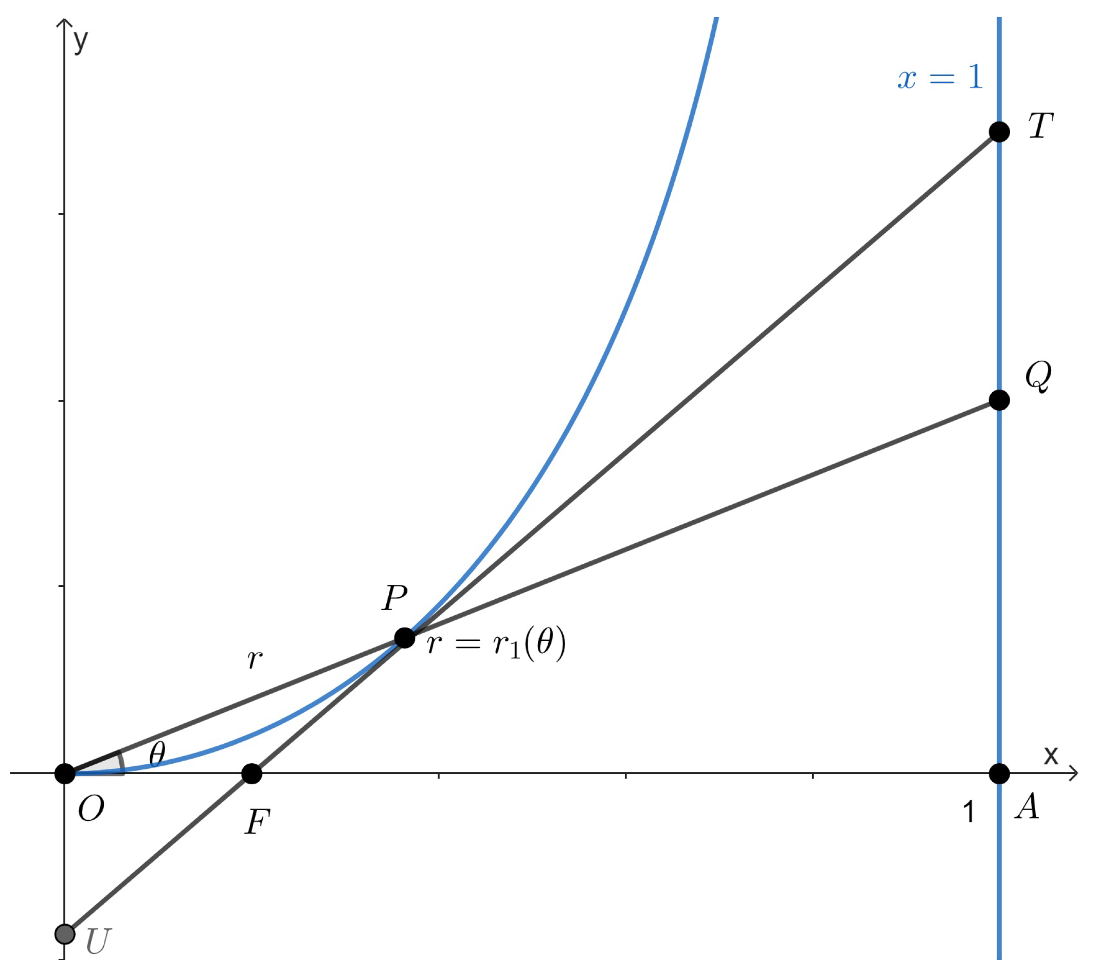
Suppose that the tangent line of the curve Equation (4) at the point P intersects x-axis, y-axis, and the line at points F, U, and T, respectively (see Figure 1). Then,
- 1
- ,
- 2
- ,
- 3
- ,
- 4
- ,
where x is the abscissa of point .
Proof.
The equation of line is . By substituting in this equation, we can find the coordinates of point . The equation of tangent line is . By substituting , , and in this equation, we can find the coordinates of points F, U, and T, respectively:
We can now find
It remains only to put these formulas in the required equalities to check that each of the first three equalities is equivalent to Equation (4). The fourth part follows from the previous equalities and the sine theorem for . □
It is also possible to prove these geometric properties using plane geometry methods, which we discuss in Section 4. Using these plane geometry methods, one can also prove the following geometric property.
Theorem 2.
The radius of the circle through O and tangent to line at point P is equal to the radius of the circle through O and tangent to line at point Q (see Figure 1).
Proof.
The center of the circle through O and tangent to line at point P is the intersection of perpendicular bisector of line segment and line perpendicular to line at point P. We find that and . Therefore, the radius of this circle is
Similarly, the center of the circle through O and tangent to the line at point Q is the intersection of perpendicular bisector of line segment , and line perpendicular to the line at point Q. Using this, we find that the radius of this circle is . It remains only to check that by Equation (4), these radii are equal. □
The following result shows that there is a connection between the interception curve and the lemniscate functions.
Theorem 3.
The length of side and the difference of lengths of the other two sides of approach the same limit as :
where B is the second lemniscate constant.
Proof.
First, we calculate that . Since as , . On the other hand, using parametrization Equation (5), we can write
The subtrahend in the last expression approches 0 as . Therefore, it remains only to find
Since ,
By substituting , where , in the improper integral, after simplifications we obtain
We only need to show that
which follows from
Similarly,
Therefore,
□
There are other strategies for making point P follow point Q so that is smaller. However, it is possible to show that there is no optimal strategy. Consider, for example, the following scenario. Suppose that there is a barrier along line and an evader is at point . A pursuer at the origin starts to chase with a constant speed, and the evader moves with the same speed along line . It would be natural to think that the pursuer should always move toward the current position of the evader. This gives rise to a trajectory for the pursuer, commonly known as pursuit curve. However, the pursuer can also move towards a future position of the evader instead of the evader’s current position. One of the many possible ways for the pursuer to do this is to stay on the line connecting the origin with the evader. The optimal strategy for the evader is to run along barrier by never changing its direction. However, there is no optimal trajectory for the pursuer, so any candidate for the optimal curve can be improved by replacing one of its curved parts with a line segment and, therefore, shortening that part. Because of the presence of barrier , the curved part should always exist. Note that any straight line through the origin intersects , except line , which obviously can not be the optimal curve. One can pose a similar question for a sphere, where the barrier and the evader are on the great circle of the sphere, and the pursuer is at one of the poles of the great circle. This is performed in the following section.
Consider also this trajectory: first, P moves with a constant speed from O to the point with coordinates along line where , , while Q moves with the same speed from A to the point with coordinates , after which P follows Q along line and distance does not change. The value of can be made arbitrarily close to zero. On the other hand, for any chosen curve, is not possible. Indeed, , where is the projection of onto the y-axis, and is a non-decreasing function of time (or x). Therefore, for any given curve with a particular positive value of , there is always a more efficient curve making the limit even smaller. In view of these observations, it would be interesting to compare the curve in Figure 1 with the mentioned trajectory of P chasing Q, the pursuit curve.
Figure 2 was created using Maple 2022. The Maple 2022 software was also used to simplify the limits and the integrals in the paper.
Suppose now that P starts to move from O with a constant speed along such a curve that the tangent line of the curve at P always passes through Q, which moves as before with the same constant speed from A upwards along line . The obtained curve is known as the pursuit curve and defined by differential equation with initial conditions . See, for example, [16] (page 256), [3,4] (page 241 of the 1911 edition, page 607 of the 1902 edition) for the solution found by P. Bouguer in 1732:
One can check that for this curve, , and therefore , which means that the interception curve overperforms the pursuit curve in this regard.
3. Spherical Curve
We now study analogous questions for spherical geometry.
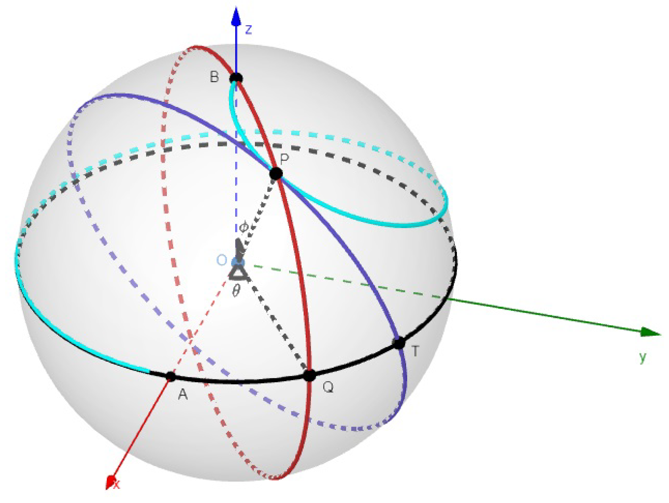
Question 2. Suppose that two points P and Q, initially at and , respectively, move with constant and equal velocity so that Q is on the great circle , of sphere with center , and P is on the great circle through B and Q of the sphere. What curve is defined by point P? (see Figure 3).
Answer. We use spherical coordinates to describe the resulting interception curve. We denote and . Since , for the coordinates of point , we can write , , and , where we assume that is a function of . Therefore, , , and . Since the points P and Q travel equal distances, by using the well-known formula from vector calculus for the length of a parametrically defined curve, we can write
where on the right-hand side of the last equality is the distance traveled by Q. By taking the derivative of both sides of Equation (6) with respect to and simplifying using the formula for , , and , we obtain with initial condition . By solving this ODE, we obtain
Note that Equation (7), which can also be written as , is sometimes called the Gudermannian function gd
. See, for example, [17], Section 4.23(viii) and [18], Section 6.12. The Gudermannian function gd
is the vertical component of the Mercator projection [19], and we see below that this connection with the Mercator projection is not a coincidence.
Theorem 4.
The points P and Q are approaching each other and
Proof.
One can observe that
and therefore the distance between the points and approaches zero as the curve winds around the sphere. □
This curve has other geometric properties. In the following, means the spherical distance between points X and Y on a sphere. For a unit sphere with center O, .
Theorem 5.
If a great circle tangent to the curve at point P of unit sphere intersects the great circle on the plane at point T (see Figure 3), then
- 1
- the sum of the lengths of the arcs and is not dependent on θ, and ,
- 2
- as θ increases, increases, decreases, and both approach to , as .
- 3
- spherical angle is equal to ,
- 4
- spherical angle is equal to .
Proof.
We continue to use the notations introduced in Question 2 and its answer. Since , we can write the following for tangent vector of curve: Equation (7)
We can find the normal vector of the plane containing the great circle through P and T, as , where :
Then, the equation of this plane is
By putting in this equation, we can find the only unknown coordinate of point in spherical coordinates:
By Equation (7), . Therefore,
which means that and consequently . Using Spherical Pythagorean Theorem ([20], page 112) for , we obtain
Therefore, , and, consequently, . Since , this proves that . Using formula and , we can now show that as increases, increases, but decreases, and both approach . Using the formula for a right angled spherical triange ([20], page 127, 4.35), we obtain
Therefore, . Similarly, . □
Using similar analytic methods, one can prove the following property of curve Equation (7) for tangent small circles. It is also possible to prove this theorem using Lemma 2.
Theorem 6.
We now discuss the mentioned connection with the Mercator projection. Let us perform a projection of the sphere onto cylinder using formula and (see [21], p. 191). Note that here, x and y are new coordinates over the cylinder [19]. Note also the difference between the spherical coordinate and latitude . Using Equation (7) and the last two equalities, we can write
Since on the cylinder, we determine that the Mercator projection of curve Equation (7) is , which is an inverse function of itself. This means that after the application of the Mercator projection, curve Equation (7) has a symmetry with respect to line (see Figure 4). Note that is a Helix on the cylinder, and it is the projection of a Spherical Spiral (a special case of loxodrom or rhumb line [1]) intersecting the meridians of the sphere at a constant angle . Since the Mercator projection is conformal (angle-preserving), the slope on the cylinder and on the sphere should be equal. Indeed, by Theorem 5,
Note that in the literature, the expression spherical spiral is sometimes used for different curves. In Figure 4, we used parametrization for this curve (red curve) ([22], Lemma 8.27), the parametrization for (orange curve), which is the Mercator projection of the previous curve onto the cylinder, parametrization for (green curve), which is the Mercator projection of interception curve Equation (7) (blue curve). Note also that in Figure 4, the stereographic projection of Equation (7) onto the plane, with respect to pole B, is a plane spiral curve (black curve), which in polar coordinates can be written as . Indeed, by Equation (7),
Line (yellow line) on the plane is the asymptote of this curve. It is known that the stereographic projection of the rhumb line is a logarithmic spiral (purple curve) ([22], Lemma 8.27). In particular, since curves and intersect at a right angle, and stereographic and Mercator projections are both conformal, the curves on the sphere, on the cylinder, and the plane in Figure 4 intersect at right angles at the indicated points. See Appendix A, Table A2 for the list of corresponding curves in Figure 4.
4. Alternative Methods for Spherical and Planar Curves
We can also prove Theorem 5 using the following lemma, which is interesting on its own.
Lemma 1.
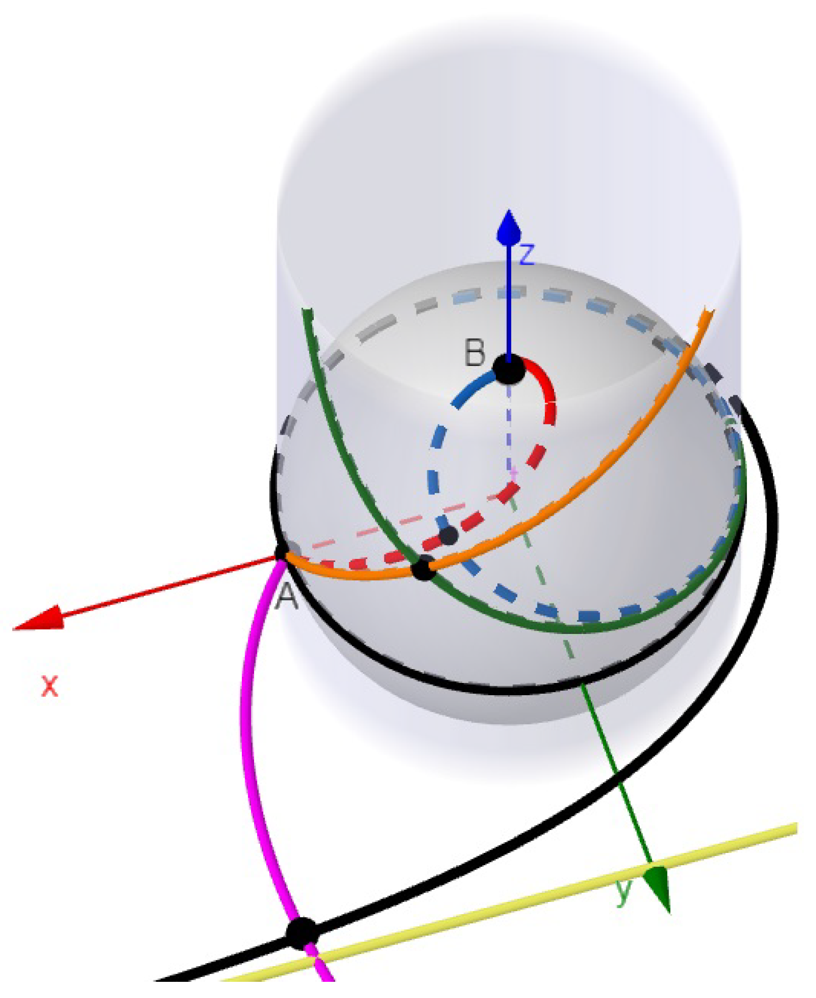
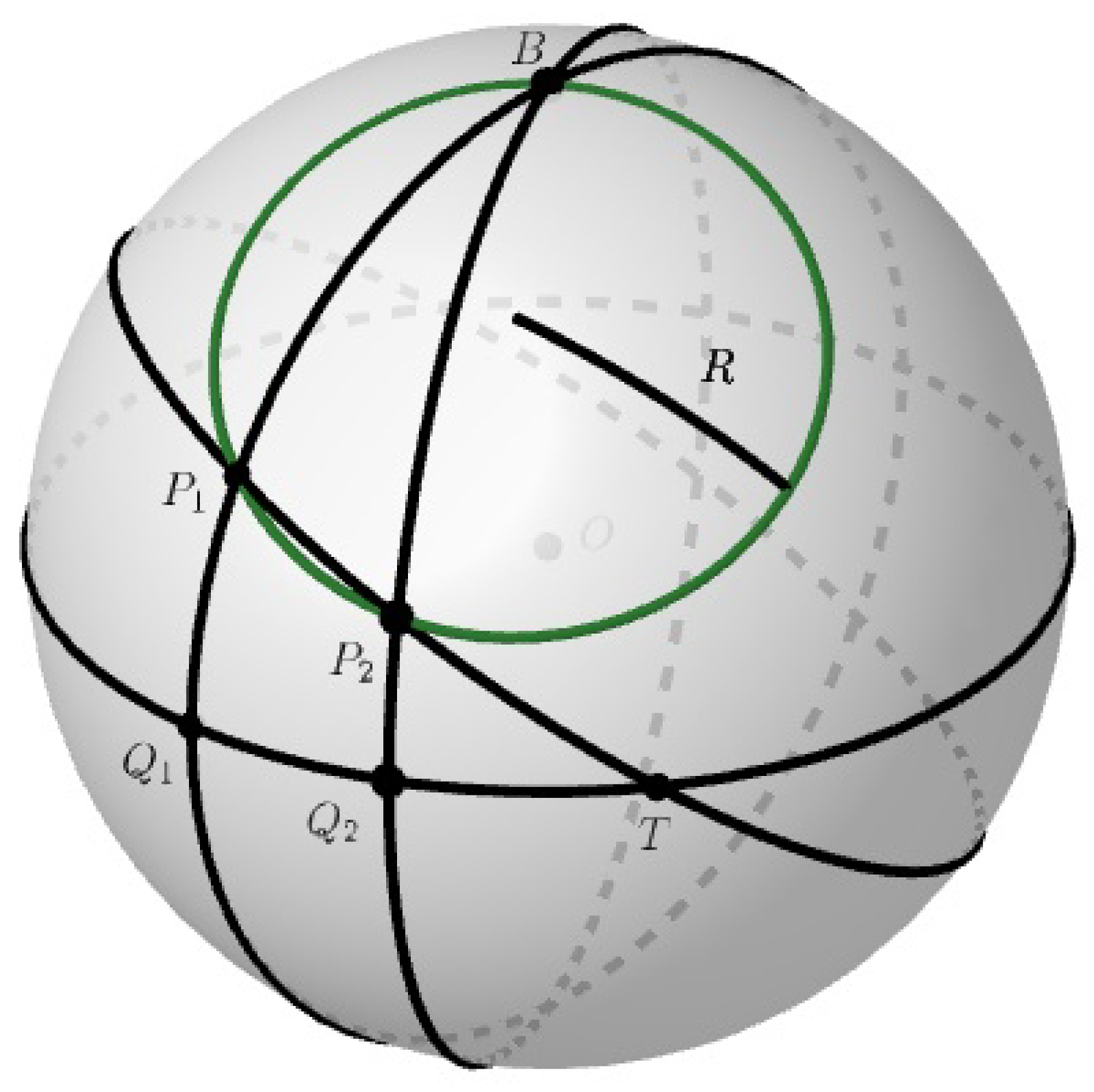
On a unit sphere with center O, a great circle and one of its poles B is drawn. Two great circles through B intersect the first great circle at and , so that . Another great circle intersects arcs and at points and so that . This great circle also intersects the first great circle at T (See Figure 5). Then,
Proof.
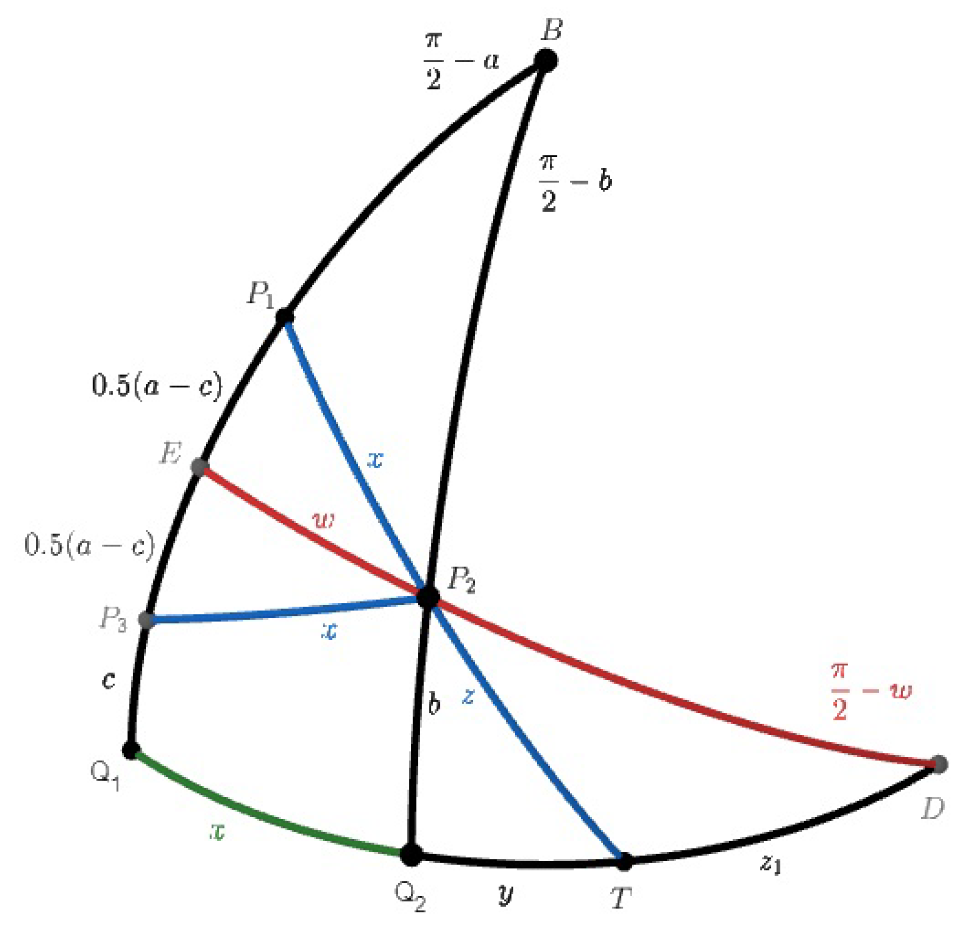
Let us denote . Since the angles at and are right angles, by the spherical sine theorem for , the angle between the two great circles at vertex B is also x ([20], page 30). , is also denoted (See Figure 6). Then, and . By the spherical sine theorem for ([20], page 115),
Since ,
We take another point on arc such that . Such a point, , should exist, because . We denote the midpoint of by E and let . Then, . Since spherical is isosceles, is its angle bisector and is perpendicular to . The three angles of the quadrilateral are right angles. Therefore, the fourth is obtuse and is acute. Since , is acute, too. Similarly, is acute. Consequently, is obtuse. Consequently, and are obtuse, and are acute. Therefore, by Equation (8), and . Similarly, and . Therefore, and . We denote the intersection of the great circles and by D. We also denote , , , . Then, and . It remains only to show that . This follows from the fact that spherical is isosceles. Indeed, and . Consequently, or . Finally,
□
For the proof of Theorem 5, one can observe that the infinitesimal line element or the length element of curve satisfies the conditions of Lemma 1 and, therefore, one just needs to pass to limit ( approaches ) which implies . Since , y and z both approach . Passing to limit also implies . Therefore, . Similarly, .
We can prove Theorem 6 using the following lemma, which is a direct consequence of the formula for the radius of the circumscribed circle of a spherical triangle (see, e.g., [23], Formula (4)).
Lemma 2.
Under conditions of Lemma 1, let a small circle of the unit sphere be circumscribed about (See Figure 5). If the radius of the small circle is R, then
It is possible to give similar simple proofs for the equalities in the planar case, too. The equalities in Theorems 1 and 2 can be proved as a limiting case of the following lemma when approaches .
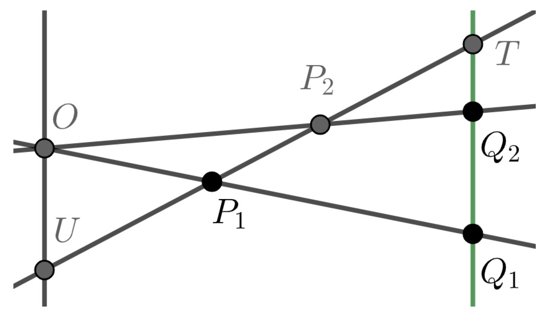
Lemma 3.
Lines passing through point O and points and on a parallel line are drawn. A line intersects these lines at U and T, and the segments and at points and , respectively, so that (see Figure 7). Then,
- 1
- and ,
- 2
- the radii of circles through points and are equal,
- 3
- if the distance between the parallel lines is 1, and the distances from points and to line are and , respectively, then
See Appendix A, Table A1 for a complete picture of corresponding lemmas.
5. Conclusions
In the paper, the two interception curves, one on a plane and the other one on a sphere, were studied. The extensive literature about the planar curve and the mentioned connections with lemnicate constants and plane geometry lemmas show that it is an important and interesting topic for mathematics and its applications. The spherical curve and its properties naturally extend these results to a geometry different from planar. The interplay between the plane and spherical geometry results and the geometric properties of curve Equations (5) and (7) were very helpful to find and prove these properties. Evident symmetry between the planar and spherical cases helped us to find more properties and shorter and more elegant proofs for them. Analogous to the planar case, there is a spherical pursuit curve studied in [24] (see also [2], page 78 of Vol. II), and it would be interesting to compare it with the spherical interception curve. It would also be interesting to consider all these questions in the context of hyperbolic geometry [24] and other planar regions [25].
Funding
This work was supported by ADA University Faculty Research and Development Fund.
Data Availability Statement
Not applicable.
Acknowledgments
I thank the reviewers and editors for their helpful suggestions and comments.
Conflicts of Interest
The author declares no conflict of interest.
Appendix A

Table A1.
Corresponding theorems in planar and spherical cases, and lemmata in Section 4 that can be used to prove these results.
Table A1.
Corresponding theorems in planar and spherical cases, and lemmata in Section 4 that can be used to prove these results.
| Plane Curve | Spherical Curve | (A)symmetry | Plane Geometry | Spherical Geometry |
|---|---|---|---|---|
| Theorem 1 | Theorem 5 | Symmetry | Lemma 3, 1. & 3. | Lemma 1 |
| Theorem 2 | Theorem 6 | Asymmetry | Lemma 3, part 2. | Lemma 2 |
| Theorem 3 | Theorem 4 | Asymmetry | - | - |
Table A2.
Corresponding curves on the sphere, on the cylinder and on the plane in Figure 4.
Table A2.
Corresponding curves on the sphere, on the cylinder and on the plane in Figure 4.
| Sphere | Cylinder Mercator Projection | Plane Stereographic Projection |
|---|---|---|
Interception curve (blue) | (green) | (black) |
Spherical spiral (red) | Helix (orange) | Logarithmic spiral (purple) |
Appendix B
In Section 2, we found parametrization Equation (5) for the curve defined by Equation (4). It is possible to write alternative parametrizations for this curve. Let us denote and . Then, from Equation (4) we obtain . Since and , we obtain a linear differential equation . Noting the initial condition , the solution of Equation (4) can also be written as
Another parametrization of the solution can be written if is solved first for x to obtain and then, noting that , a linear differential equation is obtained. Its solution offers us
References
- Weisstein, E.W. Loxodrome; From MathWorld—A Wolfram Web Resource. Available online: https://mathworld.wolfram.com/Loxodrome.html (accessed on 17 February 2023).
- Loria, G. Curve Sghembe Speciali Algebriche e Trascendenti; N. Zanichelli: Bologna, Italy, 1925; Available online: https://quod.lib.umich.edu/u/umhistmath/ABR0683.0002.001/85?rgn=full+text;view=pdf (accessed on 17 February 2023).
- Loria, G. Spezielle Algebraische und Transzendente Ebene Kurven: Theorie und Geschichte; B. G. Teubner: Leipzig, Germany, 1911; Volume 2, Available online: https://archive.org/details/speziellealgebr01lorigoog/page/n252/mode/2up (accessed on 17 February 2023).
- Loria, G. Spezielle Algebraische und Transzendente Ebene Kurven: Theorie und Geschichte. First Edition 1902. Available online: https://quod.lib.umich.edu/u/umhistmath/ABR0252.0001.001/632?rgn=full+text;view=pdf (accessed on 17 February 2023).
- Elnan, O.R.S.; Lo, H. Interception of High-Speed Target by Beam Rider Missile. AIAA J. 1963, 1, 1637–1639. [Google Scholar] [CrossRef]
- Vinh, N.X. Comment on ”Interception of High-Speed Target by Beam Rider Missile”. AIAA J. 1964, 2, 409. [Google Scholar] [CrossRef]
- Wilder, C.E. A discussion of a differential equation. Am. Math. Mon. 1931, 38, 17–25. [Google Scholar] [CrossRef]
- Zbornik, J. Akademie der Wissenschaften in Wien Mathematisch-Naturwissenschaftliche Klasse. IIa Sitzungsberichte 1957, 166, 42. [Google Scholar]
- Bailey, H.R. The Hiding Path. Math. Mag. 1994, 67, 40–44. [Google Scholar] [CrossRef]
- Kamke, E. Differentialgleichungen Lösungsmethoden und Lösungen; Springer: Wiesbaden, Germany, 1977. [Google Scholar] [CrossRef]
- Todd, J. The Lemniscate Constants. Commun. Acm (Cacm) 1975, 18, 14–19. [Google Scholar] [CrossRef]
- Todd, J. The Lemniscate Constants. In Pi: A Source Book; Springer: New York, NY, USA, 2000. [Google Scholar] [CrossRef]
- Aliyev, Y. From The First Remarkable Limit to a Nonlinear Differential Equation. In Proceedings of the 5th International Conference on Mathematics: An Istanbul Meeting for World Mathematicians ICOM, Istanbul, Turkey, 1–3 December 2021; pp. 293–304. Available online: http://icomath.com/dosyalar/2021%20P%20123.pdf (accessed on 17 February 2023).
- Cox, D.A. The Arithmetic-Geometric Mean of Gauss. L’Enseignement Mathématique 1984, 30, 275–330. [Google Scholar] [CrossRef]
- Cox, D.A. The Arithmetic-Geometric Mean of Gauss. In Pi: A Source Book; Springer: New York, NY, USA, 2000. [Google Scholar] [CrossRef]
- Savelov, A.A. Planar Curves; State Publisher of Physics-Mathematics Literature: Moscow, Russia, 1960. (In Russian) [Google Scholar]
- Olver, F.W.J.; Lozier, D.W.; Boisvert, R.F.; Clark, C.W. NIST Handbook of Mathematical Functions; Cambridge University Press: Cambridge, UK, 2010. [Google Scholar]
- Zwillinger, D. (Ed.) CRC Standard Mathematical Tables and Formulae; Advances in Applied Mathematics; CRC Press: Boca Raton, FL, USA, 2011. [Google Scholar]
- Weisstein, E.W. Mercator Projection; From MathWorld–A Wolfram Web Resource. Available online: https://mathworld.wolfram.com/MercatorProjection.html (accessed on 17 February 2023).
- Whittlesey, M.A. Spherical Geometry and Its Applications; Textbooks in Mathematics; CRC Press: Boca Raton, FL, USA, 2020. [Google Scholar] [CrossRef]
- Pearson, F. Map Projections: Theory and Applications; CRC Press: Boca Raton, FL, USA; Routledge: London, UK, 2018. [Google Scholar]
- Abbena, E.; Salamon, S.; Gray, A. Modern Differential Geometry of Curves and Surfaces with Mathematica; Chapman and Hall, CRC: Boca Raton, FL, USA, 2006. [Google Scholar] [CrossRef]
- Odani, K. On a Relation between Sine Formula and Radii of Circumcircles for Spherical Triangles. Bull. Aichi Univ. Educ. 2010, 59, 1–5. Available online: http://hdl.handle.net/10424/2951 (accessed on 17 February 2023).
- Roeser, E. Die Verfolgungskurve auf der Kugel; Dissert.: Halle, Germany, 1907. [Google Scholar]
- Morley, F.V. A Curve of Pursuit. Am. Math. Mon. 1921, 28, 54–61. Available online: https://www.jstor.org/stable/2973034 (accessed on 17 February 2023). [CrossRef]
Figure 1.
Interception curve (blue) on a Plane. Its tangent line (black), the line containing its position vector (black), and the line (blue) are also shown.
Figure 1.
Interception curve (blue) on a Plane. Its tangent line (black), the line containing its position vector (black), and the line (blue) are also shown.

Figure 2.
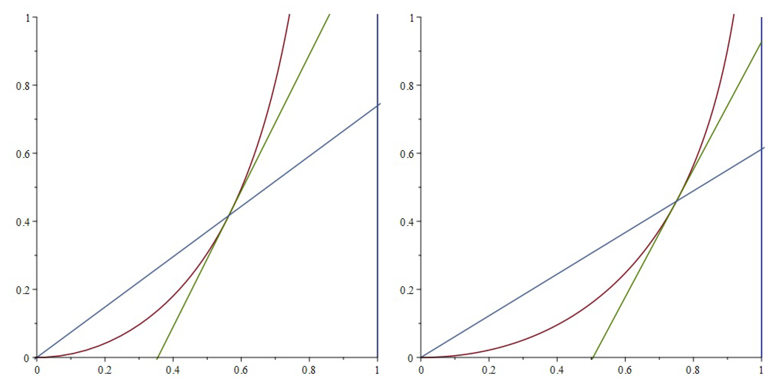
Comparison of interception (left, red) and pursuit (right, red) curves. Created using parametrization (5) and Bouguer’s formula. The tangent lines (green), the lines containing the position vectors (thin blue) of the curves, and lines (thick blue) are also shown.
Figure 2.
Comparison of interception (left, red) and pursuit (right, red) curves. Created using parametrization (5) and Bouguer’s formula. The tangent lines (green), the lines containing the position vectors (thin blue) of the curves, and lines (thick blue) are also shown.

Figure 3.
Interception curve (light blue) on a Unit Sphere. Its tangent great circle (dark blue), meridian (red) and equator (black) great circles are also shown.
Figure 3.
Interception curve (light blue) on a Unit Sphere. Its tangent great circle (dark blue), meridian (red) and equator (black) great circles are also shown.

Figure 4.
Mercator and stereographic projections of the spherical interception curve (blue) and spherical spiral (red). The other colors are explained in the text and in Appendix A, Table A1.
Figure 4.
Mercator and stereographic projections of the spherical interception curve (blue) and spherical spiral (red). The other colors are explained in the text and in Appendix A, Table A1.

Figure 5.
Lemma 1 for spherical case. The green small circle is used in Lemma 2.

Figure 6.
Proof of Lemma 1.

Figure 7.
Lemma 3 for planar case.

Disclaimer/Publisher’s Note: The statements, opinions and data contained in all publications are solely those of the individual author(s) and contributor(s) and not of MDPI and/or the editor(s). MDPI and/or the editor(s) disclaim responsibility for any injury to people or property resulting from any ideas, methods, instructions or products referred to in the content. |
© 2023 by the author. Licensee MDPI, Basel, Switzerland. This article is an open access article distributed under the terms and conditions of the Creative Commons Attribution (CC BY) license (https://creativecommons.org/licenses/by/4.0/).
Share and Cite
MDPI and ACS Style
Aliyev, Y.N. Geometric Properties of Planar and Spherical Interception Curves. Axioms 2023, 12, 704. https://doi.org/10.3390/axioms12070704
AMA Style
Aliyev YN. Geometric Properties of Planar and Spherical Interception Curves. Axioms. 2023; 12(7):704. https://doi.org/10.3390/axioms12070704
Chicago/Turabian StyleAliyev, Yagub N. 2023. "Geometric Properties of Planar and Spherical Interception Curves" Axioms 12, no. 7: 704. https://doi.org/10.3390/axioms12070704
Note that from the first issue of 2016, this journal uses article numbers instead of page numbers. See further details here.