
Bakry–Émery Curvature Sharpness and Curvature Flow in Finite Weighted Graphs: Implementation
by
 , , , and
David Cushing
1,
Supanat Kamtue
2,
Shiping Liu
3,
Florentin Münch
4,
Norbert Peyerimhoff
5,* and
Ben Snodgrass
5 1
Department of Mathematics, The University of Manchester, Manchester M13 9PL, UK
2
Yau Mathematical Sciences Center, Tsinghua University, Beijing 100190, China
3
School of Mathematical Sciences and CAS Wu Wen-Tsun Key Laboratory of Mathematics, University of Science and Technology of China, Hefei 230026, China
4
Max Planck Institute for Mathematics in the Sciences, 04103 Leipzig, Germany
5
Department of Mathematical Sciences, Durham University, Durham DH1 3LE, UK
*
Author to whom correspondence should be addressed.
Axioms 2023, 12(6), 577; https://doi.org/10.3390/axioms12060577
Submission received: 19 April 2023
/
Revised: 3 June 2023
/
Accepted: 7 June 2023
/
Published: 11 June 2023
(This article belongs to the Special Issue Discrete Curvatures and Laplacians)
Abstract
:In this paper, we discuss the implementation of a curvature flow on weighted graphs based on the Bakry–Émery calculus. This flow can be adapted to preserve the Markovian property and its limits as time goes to infinity turn out to be curvature sharp weighted graphs. After reviewing some of the main results of the corresponding paper concerned with the theoretical aspects, we present various examples (random graphs, paths, cycles, complete graphs, wedge sums and Cartesian products of complete graphs, and hypercubes) and exhibit various properties of this flow. One particular aspect of our investigations is asymptotic stability and instability of curvature flow equilibria. The paper ends with a description of the Python functions and routines freely available in an ancillary file on arXiv or via github. We hope that the explanations of the Python implementation via examples will help users to carry out their own curvature flow experiments.
MSC:
05C21; 05C50; 51K10; 53C21; 53E201. Introduction
This paper is concerned with computational aspects of a curvature flow on weighted graphs based on the Bakry–Émery calculus. This curvature flow was originally introduced in our paper [1]. The current paper focuses on properties for various concrete examples of graphs as well as stability investigations of the flow limits. Many observations in this paper are gained with the help of our curvature flow software, which is freely available as an ancillary file of [2] or via github at https://github.com/georgestagg/graph-curvature-server (accessed on 6 June 2023). A summary of our findings is presented in Section 4.
A weighted graph in this paper is a finite simple mixed combinatorial graph with vertex set V and edge set of one- and two-sided edges, together with a weighting scheme of transition rates for (which can be represented by a generally non-symmetric matrix P after an enumeration of the vertices). Transition rates can only be positive if or if there is a one- or two-sided edge from x to y. One-sided edges are denoted by ordered pairs , and two-sided edges are denoted by sets . One- or two-sided edges or with vanishing transition rates are called degenerate and a weighted graph is called non-degenerate if it does not have degenerate edges. A weighted graph is called Markovian, if we have for all . In this case, P is a stochastic matrix and we can view the transition rates as transition probabilities of a lazy random walk (with non-zero laziness if there exists a vertex with ). Our curvature flow does not affect the underlying combinatorial graph G, but it changes the weighting scheme. We will focus on a version of our flow that preserves the Markovian property. In other words, starting with an initial Markovian weighted graph , this flow will provide a family of Markovian weighting schemes with , depending on the continuous time parameter t.
Before we introduce our curvature flow, we need to briefly discuss the relevant Bakry–Émery curvature background. This curvature notion is based on the weighted Laplacian , acting on functions as follows:
The Laplacian gives rise to the following symmetric bilinear “carré du champ operators” and :
1.1. Bakry–Émery Curvature and Curvature Sharpness
Bakry–Émery curvature depends on a dimension parameter N and is well-defined at every vertex that is not isolated, that is, there exists another vertex with . For isolated vertices, there is some ambiguity on how to define their curvature, and we decided to assign to such a vertex the curvature value 0. (Another natural choice of curvature for an isolated vertex would be for all . An argument for that choice is that an isolated vertex can be viewed as a discrete analogue of a limit of round spheres with radii shrinking to 0, whose curvatures would diverge to infinity.) The definition of Bakry–Émery curvature reads as follows:
Definition 1
(Bakry–Émery curvature). The Bakry–Émery curvature of a non-isolated vertex for a fixed dimension is the supremum of all values , satisfying the curvature-dimension inequality
for all functions . We use the simplified notation and . We denote the curvature at by . If is isolated, that is, we have for all , we set for all .
This curvature notion is motivated by Bochner’s identity (see, e.g., [3] (Prop. 4.15)), a fundamental pointwise formula in the smooth setting of n-dimensional Riemannian manifolds involving gradients, Laplacians, Hessians, and Ricci curvature. It was introduced for the smooth setting in [4]. The curvature was then reintroduced several times in the setting of graphs, see [5,6,7]. For further research about Bakry–Émery curvature on finite graphs, see, e.g., [8,9,10,11,12,13,14,15,16,17,18,19].
By the definition, the inequality
holds for every function f, and therefore, also holds for the combinatorial distance function . Here, is the length of a shortest directed path from x to y (if there is no such path, we set ). If we have equality at x in (2) for this particular function , we say that the vertex is N-curvature sharp. Curvature sharpness will be particularly important in our considerations. Curvature sharpness was originally introduced in [20] (Definition 1.4). The (equivalent) definition given in this paper is inspired by [21] (Proof of Theorem 1.2). For more details about relations between different curvature sharpness definitions see Section 3 of [1].
Definition 2
(Curvature sharpness). Let be a weighted graph and . A vertex is called N-curvature sharp if we have
for the distance function . Moreover, a vertex is curvature sharp if it is curvature sharp for some dimension . A weighted graph is called curvature sharp, if every vertex of G is curvature sharp.
Note that each function with gives rise to an upper curvature bound via the inequality (2). Namely, we have
A vertex is therefore N-curvature sharp if its Bakry–Émery curvature agrees with the specific upper curvature bound . We would also like to mention the following monotonicity property of curvature sharpness: If is N-curvature sharp that this vertex is also curvature sharp for any dimension (see [1] (Prop. 3.1)).
In the next subsection, we present an important reformulation of Bakry–Émery curvature at using a specific matrix , which will be important in the definition of the curvature flow.
1.2. Reformulation of Curvature via a Schur Complement
The combinatorial distance function allows us to define distance spheres and distance balls,
Let be a non-isolated vertex. It turns out that the Bakry–Émery curvature is determined locally, that is, can be derived solely from the information about the 2-ball
More precisely, denoting and , there exist a column vector and a symmetric matrix of size m and a symmetric matrix of size such that, for functions with ,
where and
and , accordingly. Using the -block decomposition
and employing the Schur complement
for matrices with positive semidefinite -blocks with the pseudoinverse of A (for a given matrix , its pseudoinverse is defined by the following conditions: , , and and are both symmetric matrices), we can reformulate Bakry–Émery curvature at for dimension as follows (see Section 2.4 in [1]):
Let be a non-isolated vertex. is then the maximum of all such that
where means that is positive semidefinite.
This curvature translation was motivated originally by the aim to reformulate the computation of Bakry–Émery curvature as an eigenvalue problem (see [22,23,24]).
The symmetric matrix of a non-isolated vertex is of size m and is—in the non-degenerate case—closely related to another symmetric matrix , which, in turn, can be viewed as a discrete counterpart of the Ricci curvature tensor at a point of a Riemannian manifold (see formula (1.2) and Section 7 in [24]). In the case of a Markovian weighted graph, curvature sharpness at a vertex can also be alternatively expressed with the help of the matrix as follows.
Theorem 1
(see Theorem 1.3 in [1]). Let be a Markovian weighted graph and be a non-isolated vertex with . Then, the following statements are equivalent:
- (1)
- x is curvature sharp;
- (2)
- x is curvature sharp for dimension ;
- (3)
- We havewhere and is the all-one column vector of size m.
1.3. Curvature Flow
Let be a fixed initial weighted graph with . For every non-isolated vertex , the size of the corresponding symmetric matrix agrees with the degree of the vertex x, that is, the number of one- and two-sided edges emanating from x, and the entries of are determined by the transition rates of edges of the 2-ball . Our curvature flow associates to this initial data a smooth matrix-valued function with . The corresponding symmetric Q-matrices at time depend on the weighting schemes , and we denote them henceforth by for all . Our curvature flow is now defined as follows.
Definition 3
(Curvature flow). Let be a finite weighted graph. The associated curvature flow is given by the following differential equations for all non-isolated vertices and all :
where and
In the case of an isolated vertex , its curvature flow is given by the simple equation , that is is a constant function in t.
We note that the curvature flow Equation (6) guarantees that the diagonal entries of the weighting scheme do not change. The functions in the curvature flow Equation (7) play the role of a normalization since, for the choice , various transition rates will be unbounded as the time parameter increases. Note that in the smooth case of closed Riemannian manifolds , a suitable normalization leads to volume perseverance of under the Ricci curvature flow. Our aim is to preserve the Markovian property, and it was shown in our first paper that the curvature flow preserves this property if we choose the normalization functions
Let us give the explicit formulas for the curvature flow Equation (7) for this particular choice of , where always represent vertices in (see [1] (Formula (66)):
Here, we use . Note that (6) guarantees that is independent of the time parameter t.
The following theorem collects some fundamental properties of the normalized curvature flow.
Theorem 2
(see Theorem 1.5 and Prop. 1.6 in [1]). Let be a Markovian weighted graph. Then, the curvature flow associated with with normalization (8) is well defined for all and preserves the Markovian property. If is non-degenerate, then is also non-degenerate for all . Moreover, if the flow converges for to , then the weighted graph is curvature sharp.
We would like to emphasize that, even in the Markovian case, a flow limit of a non-degenerate weighted graph is in most cases no longer non-degenerate, despite the fact that all weighting schemes for finite are non-degenerate. In other words, some transition probabilities converge to zero under our normalized curvature flow, as time tends to infinity.
1.4. Other Discrete Curvature Flows
We presented already other curvature flows in [1] and briefly recall them here for the readers’ convenience.
To our knowledge, the curvature flow on discrete Markov chains in this paper is the first one that is based on Bakry–Émery curvature. Other curvature flow investigations for discrete Ricci-type curvature are the following:
2. Curvature Flow Examples
In this section, we investigate normalized curvature flows on some unmixed combinatorial graphs . By unmixed we mean that G does not have one-sided edges. We assume in all examples and statements in this section that our graphs are finite, simple, unmixed, and connected and that our initial weighting schemes are non-degenerate Markovian without laziness (even if we do not mention this). Curvature flow limits with are necessarily curvature sharp by Theorem 2 above. We do not know of any initial Markovian weighted graph that does not converge as . Moreover, we know that every finite connected graph with at least two vertices admits many curvature sharp Markovian weighting schemes without laziness (see [1] (Theorem 1.10)). These facts give rise to the following conjecture.
Conjecture 1
Let us now address some practical aspects of the curvature flow implementation. The Python code is freely available as an ancillary file of [2] or via github at https://github.com/georgestagg/graph-curvature-server (accessed on 6 June 2023). The solution of the curvature flow is computed numerically by the Runge–Kutta (RK4) method, which is based on a time discretization with time increments . In the following examples, we choose the step sizes and . In order to distinguish between the theoretical curvature flow and its implementation, we refer to the latter as the numerical curvature flow. Since a numerical curvature flow cannot run forever, a suitable numerical convergence criterion needs to be introduced. Our convergence criterion is based on the parameter . We say that a numerical curvature flow solution has converged numerically at time t (with respect to the parameter ) if all the entries of differ from the corresponding entries of and by less than . The numerical flow limit is then defined to be . In all the following examples, we set .
In this section, we are particularly interested in numerical flow limits that are not numerically totally degenerate. An unmixed weighted graph is called numerically totally degenerate if there are no edges with numerical non-zero transition rates in both directions, where we consider a transition rate as numerically non-zero (with respect to a parameter ), if and only if . In all the following examples we set .
2.1. Random Graphs
In this subsection, we investigate the numerical curvature flow for random weighted graphs with vertex set V. The relevance of this example is that it provides insights into flow limits for general graphs without any special symmetries. At the same time, readers are familiarized with our software tool, enabling them to run examples of their own interest. The edge set E of the random graph G is generated by an Erdös-Rényi process [37], that is, any pair of vertices is independently and randomly connected by a two-sided edge with a probability . Similarly, we choose a random initial weighting scheme with the property that all non-zero transition rates lie in the interval , for some positive parameter . We are interested in the properties of the numerical flow limits of these graphs. If the parameter in the Erdös-Rényi process is too small, these flow limits are always numerically totally degenerate. A reasonable choice to obtain not numerically totally degenerate flow limits for such random graphs with, say, 10 vertices in roughly half of the cases, is .
Example 1
(A random graph with 10 vertices). Let be the unmixed weighted Markovian graph with vertex set and
This randomly generated initial graph is illustrated on the left-hand side of Figure 1. The numerical curvature flow of has numerical convergence time (with respect to ). The numerical flow limit is presented on the right hand side of Figure 1. Let us briefly explain the illustration of the edges of this flow limit: Edges with numerical non-zero transition rates in both directions are displayed in green. Edges with only one-sided numerical non-zero transition rates are displayed as dashed red lines with arrows. Edges whose transition rates shrink in both directions numerically to zero under the curvature flow are displayed as dotted black lines. The corresponding non-zero transition rates are written along these edges. The vertices of the green edges of the flow limit in Figure 1 are given by
Since there are no numerical non-zero transition rates from these vertices to the other vertices , the vertex set W together with the green edges and their transition rates represent a highly connected non-degenerate Markovian weighted subgraph . The combinatorial graph with vertex set W can be viewed as a double cone over the complete graph of the four vertices with the vertices as its cone tips. The transition rates of the weighting scheme towards all vertices in are , all transition rates towards are and all transition rates towards are . Note that such a weighted double cone over with these transition rates for any choice of satisfying is curvature sharp (this follows readily from the geometric criterion in [1] (Theorem 3.15), since the weighting scheme is volume homogeneous in all vertices and reversible with , and ). Therefore, not only is the flow limit itself curvature sharp in Theorem 2 but also the highly connected non-degenerate weighted subgraph .
Figure 2 presents the transition rates of the vertices under the curvature flow as functions over the interval . While most transition rates converge to strictly positive limits, the transition rates and shrink to zero. Consequently, the corresponding edges on the right-hand side of Figure 1 are represented by a dashed red line and a black dotted line, respectively.
Let us finally consider the curvatures of the vertices under the curvature flow. We focus primarily on the vertices and and the dimension parameter . Figure 3 presents the ∞-curvature (in blue) and upper curvature bound (in orange) of as functions over the interval . Note that the absence of laziness implies that the upper curvature bounds are all (see [1] (19)). For both vertices, the curvature and upper curvature bound functions are numerically asymptotic as , indicating that and of the flow limit are ∞-curvature sharp. (In fact, all vertices in this example are ∞-curvature sharp with respect to the flow limit.) This is not always the case, but Theorem 1 confirms that all vertices of a flow limit are at least N-curvature sharp for dimension . Moreover, the initial and final ∞-curvatures of all vertices under the curvature flow are presented in Table 1. The final curvatures of all vertices in assume the highest values , followed by the final curvature values and of the vertices and , respectively. All other vertices in have much lower final curvatures with values .
Example 1 and its illustrations were generated by the following code.
![Axioms 12 00577 i001]()

Let us explain the commands of this program in detail. After initializing various parameters in lines 1–11, a random graph is generated in line 13 via an Erdös-Renyi process with probability . A corresponding random non-degenerate Markovian weighting scheme without laziness is generated in line 14, with each non-zero transition rate satisfying . The numerical convergence time is determined in lines 16–18. In most cases, the convergence time does not exceed 100. (If convergence is not achieved by , the curvature flow computation stops at that time and notifies the user.) The numerical curvature flow on the interval is solved again in line 21. Initial and final weighting schemes are displayed by the commands in lines 23 and 24, respectively, providing the illustrations given in Figure 1. The transition rates of the vertices and are displayed by the command in line 25, providing the illustrations given in Figure 2. The curvatures and upper curvature bounds at time steps , , are computed in lines 27 and 28, respectively, with the choice . They are displayed for the vertices and via the command in line 29, providing the illustrations given in Figure 3.
When running this program, users may be faced with the following message:
‘norm_tolerance’ has been exceeded at one or more vertices, at time t = … Would you like to:
A = Stop calculation and return list of P-matrices so far
B = Apply manual normalization now, and apply it again when necessary without asking (you will still be notified when it is applied)
C = Apply manual normalization now, and ask again before reapplying it
Please enter A, B or C here:
The reason behind this message is the following. The computation of the numerical curvature flow is based on a time discretization. Therefore, the solution will increasingly depart from the Markovian property after each time increment . If the sum of entries of one of the rows of at time t differs from one by more than , the program informs the user that a normalization of the weighting scheme is needed for the continuation of the flow calculations. After choosing the option ‘B’, the program will continue with its flow calculations without further interruptions, and the user is simply notified about the times at which the program applies further artificial normalizations of the transition rates. The user can suppress this message entirely by changing line 2 of the program into “stoch_corr = True”, in which case the program applies stochastic corrections automatically, each time with the message
Transition rates have been artificially normalized at time t = …
The numerical observations of Example 1 suggest that similar properties may also hold in general in the theoretical setting. Firstly, we call an edge in an unmixed weighted graph non-degenerate if . An unmixed weighted graph is called totally degenerate if it does not have any non-degenerate edges. Secondly, we denote the vertices of all non-degenerate edges of a flow limit by , and denotes the subgraph of G consisting of the vertices W and all non-degenerate edges of . Moreover, denotes the restriction of the weighting scheme to the vertex set W. We call the non-degenerate subgraph of and we conjecture the following:
Conjecture 2.
If the normalized curvature flow of a nondegenerate unmixed Markovian weighted graph converges to a not totally degenerate limit , then the non-degenerate subgraph coincides with the induced subgraph (of G) of the subset and all transition rates from W to are zero. is a non-degenerate Markovian weighted graph, which is itself curvature sharp.
Figuratively speaking, the curvature flow converges towards the non-degenerate Markovian subgraph consisting of highly connected components. Moreover, each vertex of is usually connected to the set W by a sequence of edges with one-sided non-zero transition rates pointing towards the set W, and we generally expect that the ∞-curvature values of the vertex set W in are significantly larger than the ∞-curvature values of the set in .
In Example 1, the weighted Markovian subgraph has only one connected component, but we will see in the next subsection in the case of paths and cycles that may be composed of more than just one connected component.
2.2. Paths and Cycles
Paths and cycles are the easiest examples of graph families and are therefore natural examples to study. We will see that both families have flow limits of very similar types. Let be a path of length , that is, with a two-sided edge between and if and only if . If , G is a trivial case of a star graph and any Markovian weighting scheme satisfying and is curvature sharp (see [1], Example 4.3). For that reason, we consider only paths of lengths . A cycle of length 3 is the complete graph , and a full list of all curvature sharp weighting schemes was given in [1], Prop. 1.9, so we consider only cycles of length . The following example provides some insights into some features of curvature flow limits of weighted paths and cycles.
Example 2
(A path and a cycle of length 12). Figure 4 presents numerical curvature flow limits of a Markovian weighted path with vertices 12 vertices (left-hand side) and of a weighted cycle with 12 vertices (right-hand side). The non-zero transition rates of the initial weighting scheme for the path limit in Figure 4 were chosen as follows:
| 1 | 019 | |||||||||
| 1 |
The non-degenerate subgraph of the path limit consists of as its vertex set together with the four green edges. Moreover, has two paths of length 2 as its connected components. For each vertex , there exists a directed path to one of the components of via a sequence of one-sided transition rates. For example, the vertices are connected to the vertex via such one-sided paths, and are connected to the vertex via such one-sided paths.
The cycle limit on the right-hand side of Figure 4 is totally degenerate with no green edges, and all one-sided non-zero transition rates are oriented in a clockwise direction. The experiments show that Figure 4 exhibits generic limit properties: flow limits of weighted paths are never totally degenerate and their non-degenerate subgraphs consist of disjoint paths of length . Such types of limits also appear in the case of weighted cycles. However, in contrast to the path case, sometimes a cycle limit is totally degenerate with all its one-sided transition rates oriented either clockwise or anti-clockwise. The code for running the curvature flow for paths and cycles of length n reads as follows:

Before we provide the following result about path limits, let us first introduce the notion of a two-sided degenerate edge of weighted graphs : An edge of G is called two-sided degenerate if its transition rates vanish in both directions, that is, . Similarly, an edge is called numerically two-sided degenerate, if its transition rates in both directions are . Such edges are displayed in the routine display_weighted_graph as dotted black lines (see, e.g., the edges and on the right hand side of Figure 1).
Proposition 1
(Flow limits of paths of length ). Let be a weighted path of length with consecutive vertices . Let be its corresponding curvature flow converging to a limit , such that does not have two-sided degenerate edges. Then, this limit is neither totally degenerate nor is it not non-degenerate (that is, it contains both green and dashed red edges). Moreover, the components of the non-degenerate subgraph are paths of lengths , and they are separated from each other by at least two degenerate edges. If a component of is a path of length 1, that is, just one edge , then we have .
Proof.
By the last statement of Theorem 2, we only need to prove these statements for curvature sharp weighting schemes of paths of length . Such weighting schemes can never be non-degenerate by [1] (Prop. 1.11).
For the proof that curvature sharp weighting schemes can never be totally degenerate, we note that we cannot have two consecutive degenerate edges with (since this would imply , contradicting to ). Therefore, since , any totally degenerate weighting scheme would require for any , in particular, , but this contradicts the fact that we also have and that the edge needs to be degenerate.
A curvature sharp weighting scheme cannot have more than two consecutive non-degenerate edges. This can be seen as follows: At any vertex with we must have . This follows from the arguments in the proof of [1] (Lemma 4.1) (namely, since the vertex is not contained in any triangle, we have .) If , we could iterate this argument backward and forward and would end up with the fact that all entries of the matrix P above the diagonal and below the diagonal would lie in , which is a contradiction to . So, we must have . Therefore, we cannot have two consecutive indices with , which would exist in the case of three consecutive non-degenerate edges. So, the components of are paths of length .
Moreover, any gap between two consecutive non-degenerate edges must be at least two edges: this follows from the fact that if a non-degenerate edge is followed by a degenerate edge , then we must have : if we had , then we had and, therefore, and would be non-degenerate, which is a contradiction. Similarly, if a degenerate edge is followed by a non-degenerate edge , we must have . Combining both facts implies that there cannot be a single degenerate edge separating two components of . These arguments also show that components of that are single edges must satisfy since the adjacent degenerate edges have one-sided transition rates pointing towards this component. □
Similar arguments to the above can be used to prove that for cycles, the components of any flow limit of a weighted cycle are again paths of length , unless the limit is non-degenerate. Such non-degenerate limits exist for cycles, namely the simple random walks, but experiments show that simple random walks are very unstable stationary solutions of the curvature flow. Small perturbations of simple random walks do not converge back to the simple random walk (unless our cycle is ) but converge usually to a degenerate limit. Finally, if a totally degenerate cycle limit does not have two-sided degenerate edges, then its transition rates must all be either oriented clockwise or anti-clockwise; otherwise, we would necessarily have a vertex with transition rates of both incident degenerate edges pointing towards this vertex. This would fail to satisfy the Markovian condition at this vertex.
Paths and cycles of length have the property that no edge is contained in a triangle. We would like to finish the section with a general statement about the curvature flow for edges not contained in triangles.
Proposition 2.
Let be a weighted Markovian graph without laziness and be its associated normalized curvature flow. If we have, for some and an edge , and e is not contained in a triangle of G, then we have
2.3. Complete Graphs
Complete graphs are the natural choice for the study of the behavior of curvature flows of highly connected graphs. For these graphs, the simple random walks turn out to be the flow limits of non-degenerate initial weighting schemes. The simple random walk on any complete graph is a non-degenerate curvature sharp Markovian weighting scheme. Our experiments show that any non-degenerate initial weighting scheme on converges to the simple random walk, that is . The following example shows that convergence to the simple random walk appears even if the initial weighting scheme is degenerate. This is not in contradiction to Proposition 2 since, in a complete graph , , every edge is contained in a triangle. Example 3 is the only exception in this section where we allow an initial weighting scheme to have degenerate edges.
Example 3
(A degenerate weighted complete graph with six vertices). Let be the complete weighted Markovian graph with vertex set and
as illustrated in Figure 5. Note that the edges and of this initial weighting scheme are degenerate, with the latter being two-sided degenerate. The numerical curvature flow has numerical convergence time (with respect to ) with the simple random walk as its numerical flow limit. Figure 6 presents the transition rates of the vertices and . Of particular interesting are the functions and for , since their initial values are zero.
Based on our experiments, we conjecture the following, which is a strengthening of [1] (Conjecture 1.8).
Conjecture 3
(Curvature flow of complete graphs). Let be a Markovian weighting scheme without laziness on a complete graph with such that, for every proper subset , there exist and with and . Then, the curvature flow has a limit , which is the simple random walk.
2.4. Wedge Sums of Complete Graphs
Let and be two combinatorial graphs and and . By merging the vertices and into one new vertex x, which inherits the incident edges of both vertices and , we obtain a new combinatorial graph in which we denote the wedge sum of and . In this subsection, we consider the flow limits of wedge sums of complete graphs. The study of these graphs leads to an interesting dynamical aspect of our curvature flow, namely that its limits concentrate on one of the components of these wedge sums.
Example 4
(A wedge sum of a , , , and ). We consider the curvature flow on the wedge sum of complete graphs presented in Figure 7 with random initial weighting schemes . The adjacency matrix A of this graph is generated with our code in the following way:![Axioms 12 00577 i003]()

Our experiments show that, depending on the initial weighting scheme , the curvature flow converges to a limit that is concentrated in one of the complete graphs. More precisely, the limit weighting scheme represents a simple random walk on one of the complete graphs while, from all other vertices, there is a directed path of transition rates towards this particular complete graph. Figure 8, Figure 9 and Figure 10 show the numerical curvature flow limits of various random initial weighting schemes. We carried out several runs of 100,000 numerical curvature flows with random initial weighting schemes to describe the limit behavior of these flows quantitatively. The results are presented in Table 2. While more than of limits concentrate on the largest clique , it is somewhat surprising that more limits concentrate on than on the larger subgraph . Not a single flow limit ended up concentrating on . The mean numerical convergence time is shortest for , followed by and (with respect to ). While most convergence times are below 100, there were maximal numerical convergence times well above 500.
The limit behavior described in the above example seems to be common for many wedge sums of complete graphs. It is, however, not always true that flow limits concentrate on just one of the constituents of a wedge sum. A path of length can be viewed as a wedge sum of consecutive ’s, and we have seen in Section 2.2 that flow limits will concentrate on more than only one of these ’s (see left-hand side of Figure 4). Another special case of a wedge sum is a dumbbell which is our next example.
Example 5
(A symmetric weighted dumbbell). The weighted graph in this example is a wedge sum of a , and another , together with a simple random walk as initial weighting scheme (see line 4 in the code). This situation can be set up by the following code:![Axioms 12 00577 i004]()

The numerical convergence time is 79 and the limit of the numerical curvature flow concentrates on the “bridge” between the two ’s, as illustrated in Figure 11. (To obtain the flow limit illustrated at the right-hand side of this figure, users should choose .)
This limit could have been predicted assuming that the initial weighted graph symmetry across the “bridge” is preserved under the curvature flow and that the limit concentrates on only one of the complete graphs . If instead of the simple random walk, a random initial weighting scheme would have been chosen on the dumbbell G, the limit would have usually concentrated on one of the two ’s.
2.5. Cartesian Products of Complete Graphs
It is tempting to assume that simple random walks are always the preferred curvature flow limits in relation to complete graphs. However, this is not always the case as the following example shows. Namely, we have the following result for Cartesian products of complete graphs:
Theorem 3.
Let G be the Cartesian product of two complete graphs and with the non-lazy simple random walk P as the initial weighting scheme. Then, the curvature flow converges to a limit as with limit transition rates
where are the transition rates along edges between and with , and (“horizontal edges”), and are the transition rates along edges between and with and , (“vertical edges”).
Proof.
By symmetry of the configuration, we have only two types and of transition rates for the curvature flow at time (for horizontal and vertical edges, respectively) with
and
due to the Markovian property. This implies that and , and we only need to consider an ordinary differential equation for a with initial condition . We can also assume without loss of generality that . We derive from the explicit description (9) of the curvature flow that
If this differential equation converges as , its limit must satisfy
that is
with
Our assumption implies that we have
and that the right hand side of (10) is strictly positive for in the interval
zero at , and strictly negative for on the interval
These monotonicity properties force the function to converge to the limit . □
Example 6
(Flow limit of with simple random walk). The following code computes the numerical flow limit for with the simple random walk as initial weighting scheme.

The initial transition rates are all equal to , and the transition rates of the numerical limit are and , as predicted by the above theorem.
2.6. Totally Degenerate Flow Limits
As mentioned before, many curvature limits are totally degenerate. Therefore, it is worth investigating the properties of those particular limits.
Example 7
(The octahedron with a totally degenerate flow limit). Let with be the unmixed graph representing the octahedron, as illustrated in Figure 12 (left hand side). While the simple random walk without laziness is a stationary solution of the normalized curvature flow, any small perturbation of this initial weighting scheme leads to another curvature sharp limit, which is totally degenerate. For example, the initial weighting scheme
converges to the totally degenerate limit illustrated in Figure 12 (right-hand side) under the numerical curvature flow.
The following considerations show that the limit in Example 7 is essentially the only totally degenerate curvature sharp weighting scheme without two-sided degenerate edges for the octahedron (see Proposition 3 below). We start with a general unmixed combinatorial graph without isolated vertices. A totally degenerate weighting scheme P assigns to each edge either a direction ( if and if , illustrated by a red dashed line with an arrow) or the edge is two-sided degenerate (that is , illustrated by a black dotted line). A first observation is that none of the vertices can be a sink: the Markovian property requires that at least one edge incident to x must be outward directed. The following lemma presents a useful property of triangles.
Lemma 1.
Let be a totally degenerate curvature sharp Markovian weighted graph without laziness. Then, the directions of a triangle without two-sided degenerate edges cannot be oriented, that is, its edges cannot have the orientations or .
Proof.
Assume that a totally degenerate curvature sharp Markovian weighting scheme without laziness contains a triangle with , that is, we have an orientation . This means, in particular, that . We can read off the flow equation (9) that curvature sharpness of a totally degenerate Markovian weighting scheme means
Since we have , this means
in contradiction to . The orientation can be ruled out similarly. □
The main tool in the proof of the following proposition can be found in [38] (Exercise 25.14). Assume a tessellation of the two-dimensional sphere carries an orientation along all its edges. For every vertex v of the tessellation, let , where is the number of changes in the orientation of edges adjacent to v (in cyclic order). For a face f, let , where is the number of changes in the orientation (clockwise vs. anti-clockwise) of edges of f. Then, we have
Proposition 3.
Let be the octahedron, as illustrated in Figure 12 (left-hand side). Then, G has essentially only one totally degenerate non-lazy curvature sharp Markovian weighting scheme without two-sided degenerate edges, namely, we have (up to a permutation of the vertices corresponding to a graph automorphism)
and
Proof.
We can think of the octahedron as a tessellation of the sphere by eight triangles, all of them not oriented, by Lemma 1. This means that for all faces of the octahedron. Therefore, we must have
that is, at least two vertices of the octahedron must have , which means that each of them must be a source or a sink. The Markovian property rules out sinks, and two sources cannot be adjacent (otherwise they would be connected by a non-degenerate edge). Therefore, the octahedron must have two sources at distance 2, which we denote by . Their edges are all directed towards a cycle of length 4. The directions of the edges in this cycle must be directed, for otherwise there would be a sink in this cycle, which is not possible. We denote this oriented cycle by , and we must have
where we used the notation for simplicity. Applying formula (12) to yields
that is . Similarly, we can show that all transition rates must coincide and, therefore, . The same arguments apply to the vertex , finishing the proof of the proposition. □
Conjecture 4
(Flow limits of the octahedron). The normalized curvature flow on the octahedron for any non-degenerate initial weighting scheme without laziness different from the simple random walk always converges to a limit described in Proposition 3.
3. Asymptotically Stable and Unstable Curvature Sharp Markovian Weighting Schemes
Our curvature flow can be viewed as a continuous dynamical system with its limits as equilibrium states. This leads naturally to stability questions at these equilibria, which is the concern of this section. Further information about the relevance and the background theory of stability theory for dynamical systems can be found, for example, in [39] (Chapter 9).
Since every curvature sharp Markovian weighting scheme on a given combinatorial graph is a stationary solution of the normalized curvature flow, the question arises whether such a stationary solution is asymptotically stable, that is, whether any closeby Markovian weigthing scheme P converges back to this equilibrium as . This can be decided via the linearization of the curvature flow equations around such an equilibrium. In the next subsection, we will describe this linearization in full detail before we consider various examples in the following subsection.
3.1. Linearization of the Curvature Flow Equations at Equilibria
Let be a curvature sharp Markovian weighting scheme of a finite simple mixed combinatorial graph . We consider Markovian weighting schemes P near with the same laziness, that is, for all . Let . The linearization of F at the equilibrium of the normalized curvature flow is given for each component function , , by
Here, are vertices in and the potentially non-zero B-coefficients are given by
All other B-coefficients are chosen to be zero. Note, however, that the transition probabilities are not independent, and therefore, the choice of the B-coefficients is not unique, as explained in the following remark.
Remark 1.
Since we have for all , there is a degree of freedom in the choice of the B-coefficients. For example, in the case that G is an unmixed complete graph, we can replace by with arbitrary constants . This allows us to modify the B-coefficients and in (17) and (19) to vanish, and we can use instead
with
Note that in the case of the unmixed complete graph, we have and, in the formulas for the -coefficients, represent all vertices different from x, as before.
To end up with a uniquely defined Jacobi matrix of F, we need to restrict transition probabilities that are independent. For that, we introduce the subset of “essential” transition probabilities by removing, for each with outgoing directed edges, that is , one pair from . The cardinality of is , where is the subset of vertices for which we have . Any choice determines then a weighting scheme P by setting for the directed edge . Similarly, any choice also determines the parameters with by setting . Then, is a square matrix of size M, and the weighting scheme corresponding to is asymptotically stable if and only if the real parts of all eigenvalues of this square matrix are negative, and the weighting scheme is unstable if and only if at least one of the real parts of these eigenvalues is positive.
Let us reformulate this restriction in terms of matrix multiplications. We start by enumerating the vertices of the graph : . We also introduce the following enumeration on the directed edges in : Let and be the edges of the type (where second vertices are chosen with increasing indices) in , and be the edges of the type in , and so on. For all vertices with , we set and . We remove the edges from to obtain . For simplicity, we use the notation and for and , and we can write for all ,
where the last expression involves only parameters corresponding to essential directed edges . Consequently, the Jacobi matrix can be written as
where B is the square matrix of size with for , is obtained from the identity matrix by removing the rows , and with a matrix whose first columns are all the standard basis vector , the next columns are all the standard basis vector , and so on.
3.2. Examples of Asymptotically Stable and Unstable Equilibria
In this subsection, we investigate curvature sharp weighting schemes of various examples of unmixed combinatorial graphs.
Example 8
(Curvature sharp weighting schemes on a cycle). Let be a cycle of length , that is, and with indices i modulo N. For simplicity, we refer to vertex henceforth as i. We assume to be a non-lazy curvature sharp weighting scheme on , and we remove the directed edges to obtain , and the only coefficients with and , which may be potentially non-zero are (see (13)–(16)),
This implies
In the case of the simple random walk , , this simplifies to
and the corresponding matrix coincides with the adjacency matrix of whose largest eigenvalue is 2. Therefore, the simple random walk on , , is an unstable equilibrium. This is in contrast to the simple random walk on , which is asymptotically stable, as we will see in Example 10.
In the case of the totally degenerate clockwise weighting scheme and (see right-hand side of Figure 4), we have
that is, , and this curvature sharp Markovian weighting scheme is asymptotically stable. This agrees with the fact that many initial weighting schemes end up in this limit under the curvature flow. The same holds true for the corresponding totally degenerate anti-clockwise weighting scheme with and .
Example 9
(Flow limits of the octahedron). We know from Example 7 that stationary solutions of the normalized curvature flow on the octahedron are the simple random walk without laziness as well as the totally degenerate weighting scheme given as matrix in the following code (see also the right-hand side of Figure 12). The linearization is analyzed in line 10 of the program, and the function equilibrium_type with the parameters chosen in lines 6 and 7 returns one of the values (corresponding to “asymptotically stable”, ”undecided”, “unstable”, respectively), followed by a list of its eigenvalues. That is, after execution of line 10, result[0] is one of the values and result[1] is a list of the 18 eigenvalues of .![Axioms 12 00577 i006]()

The program provides us with the following list of complex eigenvalues:
| multiplicity | 2 | 2 | 2 | 2 | 2 | 2 | 2 | 4 |
This shows that the totally degenerate curvature sharp weighting scheme on the octahedron is asymptotically stable. This is expected since the initial weighting scheme in (11) of Example 7 converges to this limit under the normalized numerical curvature flow.
Running the same code for the simple random walk without laziness instead (by uncommenting line 3 and commenting out lines 4 and 5 in the above code) shows that this second curvature sharp weighting scheme is unstable. The eigenvalues, in this case, are all real-valued, one of them , and given as follows:
| 0 | |||||
| multiplicity | 3 | 3 | 2 | 6 | 4 |
Example 10
(Simple random walk on a complete graph). Let be the complete unmixed graph with vertices. Instead of the B-coefficients, we make use of the -coefficients introduced in Remark 1. The simple random walk for is a curvature sharp Markovian weighting scheme, and the non-zero -coefficients are then given by
where is an arbitrary vertex different from . Let be the vertex set of and, as in the previous example, we refer to vertex as i, for simplicity.
Let us now consider the case . The process of removing edges from described earlier leads to the following remaining edges in :
Choosing the simple random walk , we have
which is a negative definite matrix with eigenvalues , , , showing that the simple random walk on is an asymptotically stable equilibrium. This result can be numerically verified via the following code:![Axioms 12 00577 i007]()

The program returns the eigenvalues of the linearized flow matrix of at the simple random walk. Note, however, that the computed matrix is based here on the B-coefficients instead of the -coefficients, so this matrix is slightly different from the one given above, while the eigenvalues are the same.
In the case , we have and the returned matrix by the program (after changing n=2 into n=3 in line 1 of the code) is as follows:
Its eigenvalues are with multiplicity 6 and with multiplicity 2. This shows that the simple random walk on is again an asymptotically stable equilibrium.
Since numerical experiments show that all non-degenerate Markovian weighting schemes without laziness on converge to the simple random walk, we expect that the simple random walk on is an asymptotically stable equilibrium for all (see also our Conjecture 3, which is an even stronger statement). To this end, our code provides the following numerical results: The eigenvalues of for the simple random walk without laziness on the complete graph are real-valued and given by:
- with multiplicity 4, with multiplicity 6, and with multiplicity 5 for ;
- with multiplicity 5, with multiplicity 10, and with multiplicity 9 for ;
- with multiplicity 6, with multiplicity 15, and with multiplicity 14 for ;
- with multiplicity 7, with multiplicity 21, and with multiplicity 20 for .
These results give rise to the following conjecture:
Conjecture 5.
The non-lazy simple random walk on the unmixed complete graph , , is asymptotically stable and the eigenvalues of are given by
As , we have , and .
Example 11
(Simple random walks on hypercubes). We know from [1] (Corollary 1.14) that the simple random walk without laziness on a hypercube is curvature sharp, and it is the only non-degenerate curvature sharp weighting schemes without laziness if and only if d is odd. For , a non-degenerate curvature sharp weighting scheme on different from the simple random walk is given in line 4 of the following code:![Axioms 12 00577 i008]()

All eigenvalues of the corresponding linearized flow matrix provided by this code via line 6 seem to be real. Two of them are numerically zero and the other two are given by with a non-zero real λ. So this equilibrium is unstable.
Our experiments for arbitrary weighting schemes on , , close to the simple random walk show that the numerical flow converges usually to a degenerate limit. This agrees with our observation that the linearized flow matrix at the simple random walk always seems to have real eigenvalues with some of them being positive. These eigenvalues can be obtained via the following code:

Let us finish this section with a conjecture that we verified numerically for :
Conjecture 6.
The non-lazy simple random walk on the hypercube , , is unstable and the eigenvalues of the corresponding linearized curvature flow matrix are all real with the largest eigenvalue equals
4. Conclusions and Open Questions
In Section 2, we investigated curvature flows of various concrete examples. Our findings and possible directions for further research are as follows:
- (a)
- Random graphs: We observed an edge density threshold for Erdös-Rényi graphs. For values below this threshold, the flow usually converges to a totally degenerate limit, while for values above this threshold, the flow limit concentrates on a non-degenerate cluster (see Conjecture 2). Further research could encompass curvature flows of random regular graphs with simple random walks as their initial weighting schemes.
- (b)
- Paths and cycles: Our observed limits for these graphs are usually directed graphs with isolated clusters of three vertices (see Figure 4 and Proposition 1).
- (c)
- Complete graphs and their wedge sums and Cartesian products: In the case of complete graphs, non-degenerate initial weighting schemes seem to converge always to simple random walks (see Conjecture 3). In wedge sums of complete graphs, curvature flow limits usually concentrate totally on one of its components, which is most often the largest component (see Table 2). This observation might motivate further research on the largest clusters of general highly connected graphs. We also describe the flow limit of Cartesian products of complete graphs with the simple random walk as its initial weighting scheme (see Theorem 3). A natural question here is the limit behavior of Cartesian products of graphs with curvature sharp initial weighting schemes.
- (d)
- Octahedron: In the case of the octahedron, there is a unique totally degenerate flow limit (up to symmetries), which has two sources and a directed 4-cycle (see Figure 12 and Proposition 3). The shape of totally degenerate flow limits for general graphs is obscure and would benefit from further investigations.
As mentioned already in [1], curvature flow limits are always curvature sharp. A rough interpretation of curvature sharpness at a vertex is that its Ricci curvature is constant in all directions (see [1] Equation (8)). Section 3 was concerned with a dynamical aspect of these curvature flow limits, namely their stability properties. Our findings are the following:
- (e)
- Cycles: Simple random walks on cycles for are unstable, and totally degenerate directed weighting schemes are asymptotically stable (see Example 8).
- (f)
- Complete graphs: We have strong numerical evidence that simple random walks on complete graphs are asymptotically stable (numerically verified for ); see Example 10. Moreover, our numerics provide explicit information about all eigenvalues of the linearized curvature flow as stated in Conjecture 5.
- (g)
- Hypercubes: Simple random walks of hypercubes for seem to be unstable and our experiments give rise to a conjecture about the largest eigenvalue of the linearized curvature flow (see Conjecture 6).
- (h)
- Octahedron: The totally degenerate flow limit of the octahedron is asymptotically stable (see Example 9).
- (i)
- Edge-transitive graphs: In view of (e), (f), and (g), an interesting research direction would be to investigate the stability of the simple random walk for general edge-transitive graphs.
Let us end this section with some final reflections: After having introduced a discrete curvature flow based on the Bakry–Émery calculus in [1], the main concern of this paper was to gain further insights into this flow from a dynamical viewpoint using a specially developed Python software. The most pressing and still open question is whether our curvature flow is always convergent as time tends to infinity (see Conjecture 1), or whether other limiting behavior may occur such as periodic orbits. Moreover, this could be just the starting point of various further questions, for example, whether every curvature flow allows for asymptotically stable limits—a natural technique here might be to use particular Lyapunov functions (see, e.g., [39] (Section 9.3)). The dynamical viewpoint also gives rise to other questions such as the existence of heteroclinic orbits between equilibria. All these questions may lead to further research in the future.
5. Implementation of the Curvature Flow and Useful Tools
This section provides a short description of a program, written in Python, which allows users to carry out their own curvature flow experiments. This program is provided as an ancillary file of [2] or via github at https://github.com/georgestagg/graph-curvature-server (accessed on 6 June 2023) and can be used in combination with the “Graph Curvature Calculator”, which can be freely accessed at http://www.mas.ncl.ac.uk/graph-curvature (accessed on 6 June 2023).
The Graph Curvature Calculator is a powerful but easy-to-use interactive Web tool to draw graphs and to compute various types of curvatures such as Bakry–Émery curvature on its vertices or Ollivier Ricci curvature on its edges (for details see [40]). This Web tool allows users to obtain the adjacency matrix of the graph under consideration, which can then be used as input for the curvature flow code.
The curvature flow code provides functions and routines, which can be divided into six categories:
- Functions related to graphs and their adjacency matrices;
- Functions related to weighting schemes;
- Functions testing combinatorial and weighted graphs;
- Curvature flow computation routines;
- Curvature computation routines;
- Display routines.
Each category is discussed in one of the following subsections.
5.1. Functions Related to Graphs and Their Adjacency Matrices
Recall that the topology of a given Markov chain is contained in the combinatorial graph . This information is provided by the adjacency matrix of the graph. Firstly, we go through some useful functions performing operations with these adjacency matrices. Every graph generated by one of the functions below is returned as such an adjacency matrix; in particular, as a NumPy array. The names of these functions are as follows:
- rand_adj_mat(n, p, connected=False);
- complete(n);
- path(n);
- cycle(n);
- wedge_sum(A, B, i, j);
- bridge_at(A, B, i, j);
- hypercube(n);
- cart_prod(A, B);
- onespheres(A).
rand_adjmat(n, p) returns a random adjacency matrix with n vertices, where p is the probability that an edge exists between any two vertices. Therefore, higher values of p usually lead to better-connected graphs. Choosing connected=True instead guarantees that the returned adjacency matrix provides a connected combinatorial graph.
The functions complete(n), path(n) and cycle(n) return the adjacency matrix of a complete graph with n vertices, a path of length n and a cycle of length n, respectively.
wedge_sum(A, B, i, j) produces an adjacency matrix of a graph that is the wedge sum of two pointed graphs represented by the adjacency matrices A and B and the ith vertex of A and the jth vertex of B, that is, the new graph is obtained from the disjoint union of these two graphs by only identifying these two vertices and keeping all other edges and vertices disjoint.
There is also bridge_at(A, B, i, j), which returns an adjacency matrix of the graph formed by connecting the graphs represented by A and B by a single edge at the ith vertex of A and the jth vertex of B.
The function hypercube(n) returns the adjacency matrix of the n-dimensional hypercube.
The Cartesian product of two graphs represented by adjacency matrices A and B is returned by the function cart_prod(A, B). (The n-dimensional hypercube can also be alternatively generated as the Cartesian product of n complete graphs .)
Finally, for a graph given by the adjacency matrix A and the vertex set , the function onespheres(A) returns a list of lists whose i-th entry is a list of all neighbors of vertex , and whose n-th entry is a list of the combinatorial degrees of the vertices in V. This function is mainly used in the execution of other functions.
5.2. Functions Related to Weighting Schemes
The weighting scheme of a Markov chain is provided via the weighted matrix . The functions in this category are the following:
- randomizer(A, threshold=0.001, laziness=False);
- srw(A, laziness=False);
- cart_prod_prob(P, Q, p, q).
randomizer(A) and srw(A) are two useful functions that can be used to give weighted matrices from an adjacency matrix.
The function randomizer(A) returns a weighting scheme for the graph G with random, numerically non-degenerate transition rates, that is, no transition rate is chosen to be below the parameter threshold. Usually, the returned weighting schemes are without laziness, but choosing laziness=True returns weighting schemes with all vertices having laziness ≥ threshold.
srw(A) returns the weighting scheme corresponding to the non-lazy simple random walk on the graph represented by the adjacency matrix A. Choosing laziness=True, the transition rates of a vertex with degree n to its neighbors are chosen to be and its laziness is also chosen to be .
The function cart_prod_prob(P, Q, p, q) is a “weighted” analog of the function cart_prod from the previous subsection for the Cartesian product of two weighting schemes P, Q with weights p, q, with . If P and Q are of size n and m, respectively, this function returns the matrix of size , where is the identity matrix of size n and is the Kronecker product of A and B.
5.3. Functions Testing Combinational and Weighted Graphs
For combinatorial graphs given by their adjacency matrices A and weighted graphs given additionally by their weighting scheme P, we have the following test functions:
- is_connected(A);
- is_weakly_connected(A, threshold=0.001);
- is_totally_degenerate(A, P, threshold=0.001);
- is_markovian(P, norm_tolerance=0.001);
- is_curvature_sharp(A, P, norm_tolerance=0.001, threshold=0.001);
- equilibrium_type(A, P, eigenvalues=False, jacobi_matrix=False,norm_tolerance=0.001, threshold=0.001).
The function is_connected(A) returns True if and only if the adjacency matrix A represents a connected graph.
The function is_weakly_connected(P) is a “weighted” analog, which returns True if and only if the weighted matrix P represents a weakly connected graph. It does this by forming an adjacency matrix with a 1 in the th entry if and only if P[i, j] > threshold or P[j, i] > threshold and then testing for connectedness.
Recall that a weighted graph is called numerically totally degenerate if there are no two-sided edges with numerical non-zero transition rates in both directions and no one-sided edges with numerical non-zero transition rate, where we consider a transition rate as numerically non-zero if and only if threshold. The function is_totally_degenerate(A,P) tests this property.
The function is_markovian(P) tests whether the entries of each of the columns of P add up numerically to 1 up to an error .
Numerical curvature sharpness (up to an error ) of Markovian weighted graphs given by (A,P) is tested by is_curvature_sharp(A,P). If (A,P) fails to be Markovian (with respect to norm_tolerance), this function returns NONE and gives notice to the user by an error message.
For dynamical investigations of curvature flow equilibria, we have the function equilibrium_type(A,P), which always returns a list of length three. The function checks first whether (A,P) satisfies the Markovian property and is numerically curvature sharp. If this is not the case, it returns a list of three NONE values. Otherwise, the function investigates the real parts of the eigenvalues of the linearized curvature flow matrix at the equilibrium P. The first entry of the return list is or 1 depending on the maximum . If this maximum is , the return value is 1 (for “unstable”) and if this maximum is , the return value is (for “asymptotically stable”). Otherwise, the dynamical nature of the equilibrium cannot be numerically decided and the function returns the value 0. The following two entries of the return list are usually NONE unless the user made the choices eigenvalues=True or jacobi_matrix=True. In the first case, the second entry of the return list is a list of all eigenvalues of the linearized curvature flow matrix, and in the second case the third entry of the return is the linearized curvature flow matrix itself.
5.4. Curvature Flow Computation Routines
At the heart of the program are the curvature flow routines solving the initial value ordinary differential Equations (6) and (7). The relevant routines are the following:
- curv_flow(A, P, t_max, dt=0.3, C=zeroes),
- norm_curv_flow(A, P, t_max, dt=0.3, stoch_corr=True, norm_tolerance=0.001),
- norm_curv_flow_lim(A, P, dt=0.3, stoch_corr=True, norm_tolerance=0.001, lim_tolerance=0.001, t_lim=10000).
The initial Markov chain with is entered by the adjacency matrix A describing the topology of the graph G and the weighting scheme P containing the initial probability transitions .
The first routine curv_flow(A,P) computes the non-normalized numerical curvature flow with coefficients in (7). If users decide to choose other coefficient functions, they need to modify the input parameter C=zeroes. Note that zeroes(A,P) is a function returning simply a list of zeroes of length . Users can investigate modifications of the curvature flow by choosing their own coefficient functions with input values (A,P) and returning a list of length of real values. Using the discretization parameter dt=0.3 for the discrete time steps starting at t=0, the curvature flow routine creates a list P_list of weighting schemes (represented by NumPy arrays of size ) at each time increment using the Runge–Kutta algorithms RK4. There are two internal subroutines involved, which we would like to mention briefly. Pvecs_to_P translates a weighting scheme given by a list of lists (where each inner list contains the transition rates of the corresponding vertex) into the corresponding NumPy array. Pvecs_prime computes, for a given weighting scheme P, the right-hand side of the ordinary differential equations describing the curvature flow. The representation of this right-hand side is again a list of lists, as described before. The computation stops just before the discrete time steps exceed the limit time t_max and the routine returns P_list. Note that in this general setting, transition rates can assume arbitrary values and even negative ones or diverge to infinity in finite time which may lead to system error messages. Users need to be aware of this possibility.
The normalized curvature flow, using the coefficients (see (8)), is numerically computed by the routine norm_curv_flow(A,P). This special flow is the main focus of this paper and could also be mimicked by choosing C=K_inf in curv_flow. The function K_inf(A,P) returns a list of upper curvature bounds for all vertices of the Markovian weighted graph represented by (A,P) (see [1] (Formula (66)) for an explicit expression of this function in terms of transition rates). During the numerical computations of subsequent time steps, the Markovian property of the corresponding weighting schemes may be slightly violated. If this violation exceeds the threshold norm_tolerance, the routine prepares for a potential correction according to the Boolean variable stoch_corr. If stoch_corr=False, the program stops with a message to the user as discussed in Example 1. Otherwise, the program carries out the following automatic Markovian renormalization of the currently considered weighting scheme: while the diagonal entries (the laziness values) are unchanged, the off-diagonal entries in each row are rescaled by a suitable factor to guarantee that the resulting matrix becomes stochastic again. As before, this routine returns a list P_list of consecutive weighting schemes up to the time limit t_max.
While the user needs to specify the time limit t_max in the above two routines, the third routine norm_curv_flow_lim(A,P) continues computing the normalized numerical curvature flow until a numerical flow limit is reached. This limit is determined by the parameter lim_tolerance. The details for this numerical limit are explained in the introductory part of Section 2. This routine returns a list of length two: the limiting weighting scheme as a NumPy array followed by the numerical convergence time. Since it may happen that a normalized numerical flow does not converge at all (even though we are not aware of any such example), the parameter t_lim provides an upper time limit beyond which the routine will not continue. The parameters stoch_corr and norm_tolerance play the same role as in the routine norm_curv_flow.
5.5. Curvature Computation Routines
The functions in this section calculate Bakry–Émery curvatures and curvature upper bounds of graphs with given weighting schemes at all vertices.
- curvatures(A, P, N=inf, onesps=[], q=None);
- calc_curvatures(A, P_list, N=inf, k=1);
- K_inf(A, P);
- calc_curv_upper_bound(A, P_list, N=inf, k=1).
The routine curvatures(A,P) computes, for a weighted graph with and represented by (A,P), the curvatures of all vertices for dimension N and returns them as a list of length . If users are interested in curvatures for other dimensions, they need to change the parameter N=inf. There are two other inputs that can speed up the curvature calculations: if the number q of vertices in V is given, it can be specified to avoid its repeated recalculation, for example, during a curvature flow process. Similarly, if onespheres(A) has already been calculated earlier, this information can be communicated to the routine via the input variable onesps.
After a curvature flow computation with corresponding list P_list of consecutive weighting schemes, the routine calc_curvatures(A,P_list) computes the corresponding evolution of vertex curvatures by calling curvatures(A,P_list[j]) and returns it as a list of lists. Here, the j-th inner list contains the curvature evolution of the j-th vertex of the graph represented by A. The dimension parameter N=inf plays the same role as before. calc_curvatures computes curvatures only of each k-th weighting scheme provided by P_list. Where appropriate, this can help to reduce computation time.
The routine K_inf(A,P) was already discussed in the previous subsection and provides a list of upper curvature bounds for all vertices of the weighted graph represented by (A,P).
calc_curv_upper_bound is completely analogous to calc_curvatures, but it calls K_inf instead of curvatures.
5.6. Display Routines
The main display routines for users are the evolution of curvatures at various vertices during the curvature flow, the evolution of transition rates of edges emanating from vertices, and the display of individual weighted graphs with vertices arranged in a circle. The relevant routines are the following:
- display_curvatures(curv, dt=0.3, is_Markovian=True, N=inf, k=1,curv_bound=[], vertex_list=[]);
- display_trans_rates(A, P_list, dt=0.3, vertex_list=[]);
- display_weighted_graph(A, P, title=None, threshold=10**(-3),display_options=[10, True, 2, []], laziness=False).
Given the evolution of vertex curvatures during a curvature flow process via a list of lists, where the j-th inner list is the curvature evolution of the j-th vertex, display_curvatures(curv) displays the curvature evolution for each consecutive vertex separately, as illustated, for example, in Figure 3. If this information should be only given for specific vertices, this can be specified by the input parameter vertex_list. The time step dt=0.3 and the value of k together determine the labeling of the horizontal time axis. For the role of k, we refer readers to our explanation about the routine calc_curvatures. Upper curvature bounds can be inserted into the displays by the input parameter curv_bound, which needs to be given in the same format as the vertex curvatures. Constant lower and upper curvature bounds and 2 are plotted alongside if the Boolean is_Markovian is chosen to be True and if the dimension parameter N is . These bounds appear, for example, in the illustrations given in Figure 3.
Given the evolution of weighting schemes during a curvature flow process on a graph with adjacency matrix A by a list P_list of NumPy arrays, display_trans_rates(A,P_list) displays the evolution of transition rates of emanating edges for each consecutive vertex separately, as illustrated, for example, in Figure 2. The input parameters dt and vertex_list play the same role as in the previous routine.
Finally, there is the routine display_graph(A,P) with input parameters A and P representing a weighted graph . This routine produces a MatPlotLib plot of this weighted graph, with the vertices arranged counter-clockwise in a circle. The plot uses the following convention to illustrate different types of edges:
- Green, solid lines represent numerically non-degenerate edges, that is with both threshold;
- Red, dashed lines with an arrow represent numerically degenerate edges, that is, with exactly one of and strictly less than threshold;
- Black, dotted lines represent edges with numerically vanishing transition rates in both directions, that is with both strictly less than threshold.
Users can add a title to the display by specifying the input parameter title. For Markovian weighted graphs with non-vanishing laziness, the option laziness=True labels each vertex with its corresponding laziness.
The input parameter display_options of the display_graph routine remains to be discussed. This parameter is a list of four entries. The first entry determines the size of the plot. Usually, the transition rates are printed above the edges, but if the second entry is chosen to be False, this information about the transition rates is omitted. Otherwise, the transition rates are given to a number of decimal places determined by the third entry. The default positions of these transition rates are of the way along the edges, with the number closest to the vertex x in the edge being , but this can be altered manually to avoid overlapping by specification in the fourth entry of display_options. For example, if one wishes the label to be moved to a position of the way from vertex 4 to vertex 5 and the label to be moved to a position of the way from vertex 6 to vertex 2, this fourth entry should be chosen to be [[4, 5, 1/4, 1/6], [6, 2, 1/5, 1/6]].
This completes the description of the functions and routines in the accompanying Python program to this article.
Author Contributions
All authors of this paper contributed equally to the project, with the exception of the Python code, which was generated by B.S. funded by an LMS Undergraduate Research Bursary. All authors have read and agreed to the published version of the manuscript.
Funding
Shiping Liu is supported by the National Key R and D Program of China 2020YFA0713100 and the National Natural Science Foundation of China (No. 12031017). We would like to thank the London Mathematical Society for their support of Ben Snodgrass via the Undergraduate Research Bursary URB-2021-02, during which the curvature flow was implemented and which lead to many of the research results presented in this paper. David Cushing is supported by the Leverhulme Trust Research Project Grant number RPG-2021-080. Supanat Kamtue is supported by Shuimu Scholar Program of Tsinghua University No. 2022660219.
Data Availability Statement
All numerical results in this paper can be reproduced via the freely accessible Python programme. We did not store this data but generated it on the fly.
Acknowledgments
Florentin Münch expresses his gratitude for Durham University and the University of Newcastle for their hospitality and support during his UK research visit. We would also like to express our gratitude for various useful and constructive suggestions by the referees which improved the presentation of our paper.
Conflicts of Interest
The authors declare no conflict of interest.
References
- Cushing, D.; Kamtue, S.; Liu, S.; Münch, F.; Peyerimhoff, N.; Snodgrass, H.B. Bakry-Émery curvature sharpness and curvature flow in finite weighted graphs. I. Theory. arXiv 2022, arXiv:2204.10064. [Google Scholar]
- Cushing, D.; Kamtue, S.; Liu, S.; Münch, F.; Peyerimhoff, N.; Snodgrass, H.B. Bakry-Émery curvature sharpness and curvature flow in finite weighted graphs. II. Implementation. arXiv 2022, arXiv:arxiv.2212.12401. [Google Scholar]
- Gallot, S.; Hulin, D.; Lafontaine, J. Riemannian Geometry, 3rd ed.; Springer: Berlin/Heidelberg, Germany, 2004. [Google Scholar]
- Bakry, D.; Émery, M. Hypercontractivité de semi-groupes de diffusion. C. R. Acad. Sci. Paris Sér. I Math. 1984, 299, 775–778. [Google Scholar]
- Elworthy, K.D. Manifolds and graphs with mostly positive curvatures. In Stochastic Analysis and Applications (Lisbon, 1989); Progress in Probability; Birkhäuser Boston: Boston, MA, USA, 1991; Volume 26, pp. 96–110. [Google Scholar]
- Schmuckenschläger, M. Curvature of nonlocal Markov generators. In Convex Geometric Analysis (Berkeley, CA, 1996); Mathematical Sciences Research Institute Publications; Cambridge University Press: Cambridge, MA, USA, 1999; Volume 34, pp. 189–197. [Google Scholar]
- Lin, Y.; Yau, S.T. Ricci curvature and eigenvalue estimate on locally finite graphs. Math. Res. Lett. 2010, 17, 343–356. [Google Scholar] [CrossRef] [Green Version]
- Bauer, F.; Chung, F.; Lin, Y.; Liu, Y. Curvature aspects of graphs. Proc. Am. Math. Soc. 2017, 145, 2033–2042. [Google Scholar] [CrossRef]
- Chung, F.; Lin, Y.; Yau, S.T. Harnack inequalities for graphs with non-negative Ricci curvature. J. Math. Anal. Appl. 2014, 415, 25–32. [Google Scholar] [CrossRef]
- Fathi, Z.; Lakzian, S. Bakry-Émery Ricci curvature bounds for doubly warped products of weighted spaces. J. Geom. Anal. 2022, 32, 75. [Google Scholar] [CrossRef] [PubMed]
- Fathi, M.; Shu, Y. Curvature and transport inequalities for Markov chains in discrete spaces. Bernoulli 2018, 24, 672–698. [Google Scholar] [CrossRef] [Green Version]
- Hua, B.; Lin, Y. Graphs with large girth and nonnegative curvature dimension condition. Comm. Anal. Geom. 2019, 27, 619–638. [Google Scholar] [CrossRef] [Green Version]
- Ma, L. Bochner formula and Bernstein type estimates on locally finite graphs. arXiv 2013, arXiv:1304.0290. [Google Scholar]
- Man, S. Logarithmic Harnack inequalities for general graphs with positive Ricci curvature. Differ. Geom. Appl. 2015, 38, 33–40. [Google Scholar] [CrossRef]
- Pouryahya, M.; Elkin, R.; Sandhu, R.; Tannenbaum, S.; Georgiou, T.; Tannenbaum, A. Bakry-Émery Ricci curvature on weighted graphs with applications to biological networks. In Proceedings of the International Symposium on Mathematical Theory of Networks and Systems, Bayreuth, Germany, 12–15 July 2016; Volume 22, p. 52. [Google Scholar]
- Robertson, S.J. Harnack Inequality for Magnetic Graphs. arXiv 2019, arXiv:1910.04019. [Google Scholar]
- Salez, J. Sparse expanders have negative curvature. arXiv 2021, arXiv:2101.08242. [Google Scholar] [CrossRef]
- Salez, J. Cutoff for non-negatively curved Markov chains. arXiv 2021, arXiv:2102.05597. [Google Scholar] [CrossRef]
- Shi, Y.; Yu, C. Comparisons of Dirichlet, Neumann and Laplacian eigenvalues on graphs and applications. arXiv 2020, arXiv:2011.04160. [Google Scholar]
- Cushing, D.; Liu, S.; Peyerimhoff, N. Bakry-Émery curvature functions on graphs. Can. J. Math. 2020, 72, 89–143. [Google Scholar] [CrossRef] [Green Version]
- Klartag, B.; Kozma, G.; Ralli, P.; Tetali, P. Discrete curvature and abelian groups. Can. J. Math. 2016, 68, 655–674. [Google Scholar] [CrossRef] [Green Version]
- Siconolfi, V. Coxeter groups, graphs and Ricci curvature. Sém. Lothar. Combin. 2020, 84B, 67. [Google Scholar]
- Siconolfi, V. Ricci curvature, graphs and eigenvalues. Linear Algebra Appl. 2021, 620, 242–267. [Google Scholar] [CrossRef]
- Cushing, D.; Kamtue, S.; Liu, S.; Peyerimhoff, N. Bakry-Émery curvature on graphs as an eigenvalue problem. Calc. Var. Partial Differential Equations 2022, 61, 62. [Google Scholar] [CrossRef]
- Chow, B.; Luo, F. Combinatorial Ricci flows on surfaces. J. Differ. Geom. 2003, 63, 97–129. [Google Scholar] [CrossRef]
- Ollivier, Y. Ricci curvature of Markov chains on metric spaces. J. Funct. Anal. 2009, 256, 810–864. [Google Scholar] [CrossRef] [Green Version]
- Ollivier, Y. A survey of Ricci curvature for metric spaces and Markov chains. In Probabilistic Approach to Geometry; Advanced Studies in Pure Mathematics; Mathematical Society of Japan: Tokyo, Japan, 2010; Volume 57, pp. 343–381. [Google Scholar] [CrossRef]
- Ni, C.C.; Lin, Y.Y.; Luo, F.; Gao, J. Community detection on networks with Ricci flow. Sci. Rep. 2019, 9, 9984. [Google Scholar] [CrossRef] [Green Version]
- Bai, S.; Lin, Y.; Lu, L.; Wang, Z.; Yau, S.T. Ollivier Ricci-flow on weighted graphs. arXiv 2020, arXiv:2010.01802. [Google Scholar]
- Weber, M.; Saucan, E.; Jost, J. Characterizing complex networks with Forman-Ricci curvature and associated geometric flows. J. Complex Netw. 2017, 5, 527–550. [Google Scholar] [CrossRef]
- Forman, R. Bochner’s method for cell complexes and combinatorial Ricci curvature. Discret. Comput. Geom. 2003, 29, 323–374. [Google Scholar] [CrossRef]
- Topping, J.; Di Giovanni, F.; Chamberlain, B.P.; Dong, X.; Bronstein, M.M. Understanding over-squashing and bottlenecks on graphs via curvature. arXiv 2021, arXiv:2111.14522. [Google Scholar]
- Bober, J.; Monod, A.; Saucan, E.; Webster, K.N. Rewiring Networks for Graph Neural Network Training Using Discrete Geometry. arXiv 2022, arXiv:2207.08026. [Google Scholar]
- Erbar, M.; Maas, J. Ricci curvature of finite Markov chains via convexity of the entropy. Arch. Ration. Mech. Anal. 2012, 206, 997–1038. [Google Scholar] [CrossRef]
- Erbar, M.; Kopfer, E. Super Ricci flows for weighted graphs. J. Funct. Anal. 2020, 279, 108607. [Google Scholar] [CrossRef]
- Devriendt, K.; Lambiotte, R. Discrete curvature on graphs from the effective resistance. arXiv 2022, arXiv:2201.06385. [Google Scholar] [CrossRef]
- Erdos, P.; Rényi, A. On random graphs. I. Publ. Math. Debrecen 1959, 6, 290–297. [Google Scholar] [CrossRef]
- Pak, I. Lectures on Discrete and Polyhedral Geometry. 2010. Available online: https://www.math.ucla.edu/~pak/geompol8.pdf (accessed on 6 June 2023).
- Hirsch, M.W.; Smale, S. Differential Equations, Dynamical Systems, and Linear Algebra; Pure and Applied Mathematics; Academic Press: New York, NY, USA; Harcourt Brace Jovanovich, Publishers: London, UK, 1974; Volume 60. [Google Scholar]
- Cushing, D.; Kangaslampi, R.; Lipiäinen, V.; Liu, S.; Stagg, G.W. The Graph Curvature Calculator and the Curvatures of Cubic Graphs. Exp. Math. 2022, 31, 583–595. [Google Scholar] [CrossRef] [Green Version]
Figure 1.
Curvature flow of a random graph with 10 vertices with initial weighting scheme (left-hand side) and final weighting scheme (right-hand side).
Figure 1.
Curvature flow of a random graph with 10 vertices with initial weighting scheme (left-hand side) and final weighting scheme (right-hand side).

Figure 2.
Transition rates of vertices and of a random graph with 10 vertices under the curvature flow.
Figure 2.
Transition rates of vertices and of a random graph with 10 vertices under the curvature flow.

Figure 3.
Curvatures (blue) and upper curvature bounds (orange) of vertices and of a random graph with 10 vertices for the dimension ∞ under the curvature flow.
Figure 3.
Curvatures (blue) and upper curvature bounds (orange) of vertices and of a random graph with 10 vertices for the dimension ∞ under the curvature flow.

Figure 4.
Examplesof numerical curvature flow limits of a path and of a cycle of length 12.

Figure 5.
Curvature flow of a complete graph with six vertices with degenerate initial weighting scheme (left-hand side) and numerical flow limit , the simple random walk (right-hand side).
Figure 5.
Curvature flow of a complete graph with six vertices with degenerate initial weighting scheme (left-hand side) and numerical flow limit , the simple random walk (right-hand side).

Figure 6.
Transition rates of vertices and of a complete graph with six vertices under the curvature flow.
Figure 6.
Transition rates of vertices and of a complete graph with six vertices under the curvature flow.

Figure 7.
A wedge sum of a , , and a .

Figure 8.
Initial weighting scheme (left) and numerical flow limit a simple random walk on (right).

Figure 9.
Initial weighting scheme (left) and numerical flow limit a simple random walk on (right).

Figure 10.
Initial weighting scheme (left) and numerical flow limit a simple random walk on (right).
Figure 10.
Initial weighting scheme (left) and numerical flow limit a simple random walk on (right).

Figure 11.
Curvature flow of a dumbbell as a wedge sum of a , and another with simple random walk initial weighting scheme (left-hand side) and numerical flow limit concentrated on (right-hand side).
Figure 11.
Curvature flow of a dumbbell as a wedge sum of a , and another with simple random walk initial weighting scheme (left-hand side) and numerical flow limit concentrated on (right-hand side).

Figure 12.
Left-hand side: An octahedron with vertices . Right-hand side: A numerical flow limit of the octahedron with a small perturbation of simple random walk as initial weighing scheme.
Figure 12.
Left-hand side: An octahedron with vertices . Right-hand side: A numerical flow limit of the octahedron with a small perturbation of simple random walk as initial weighing scheme.


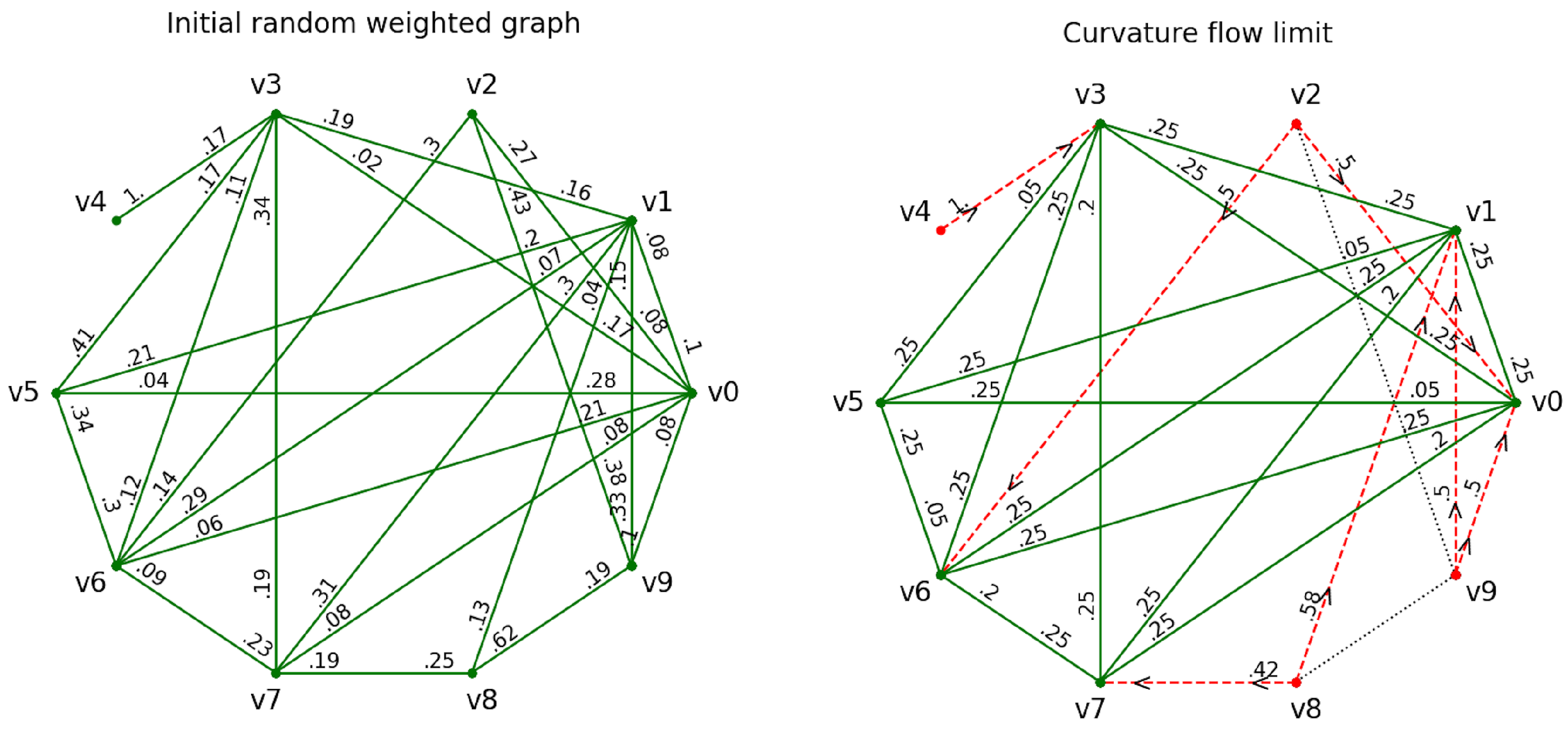
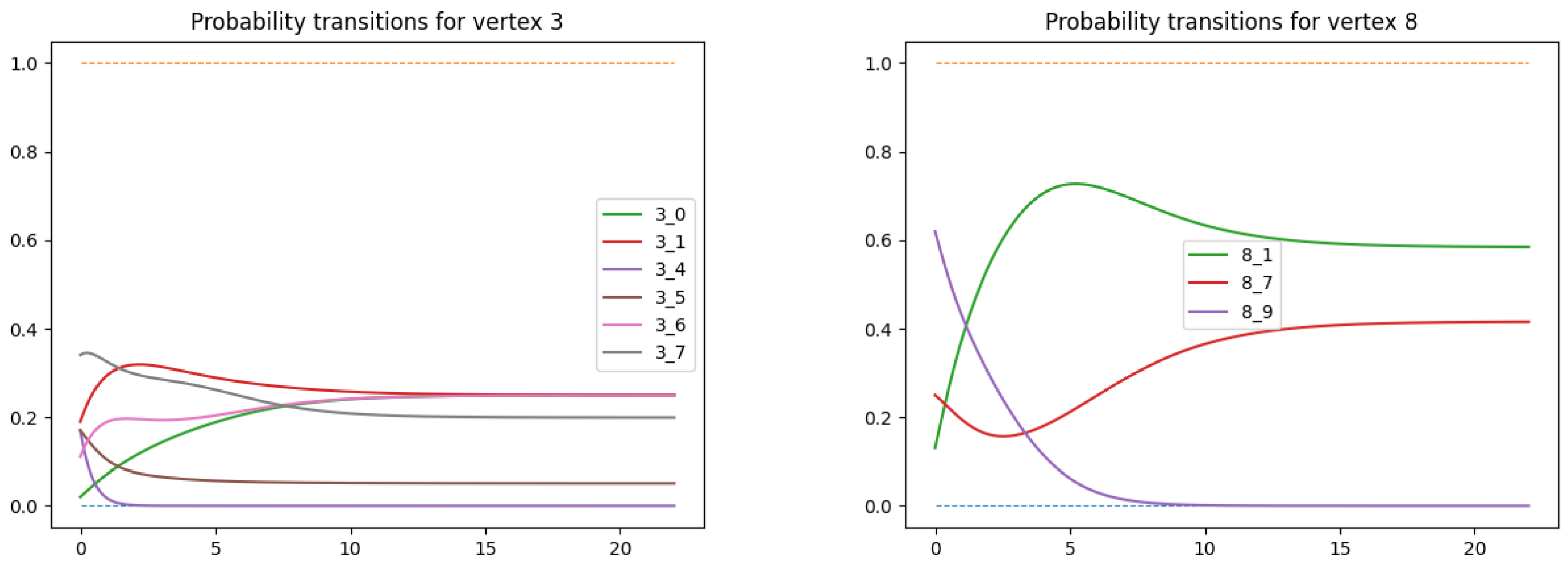
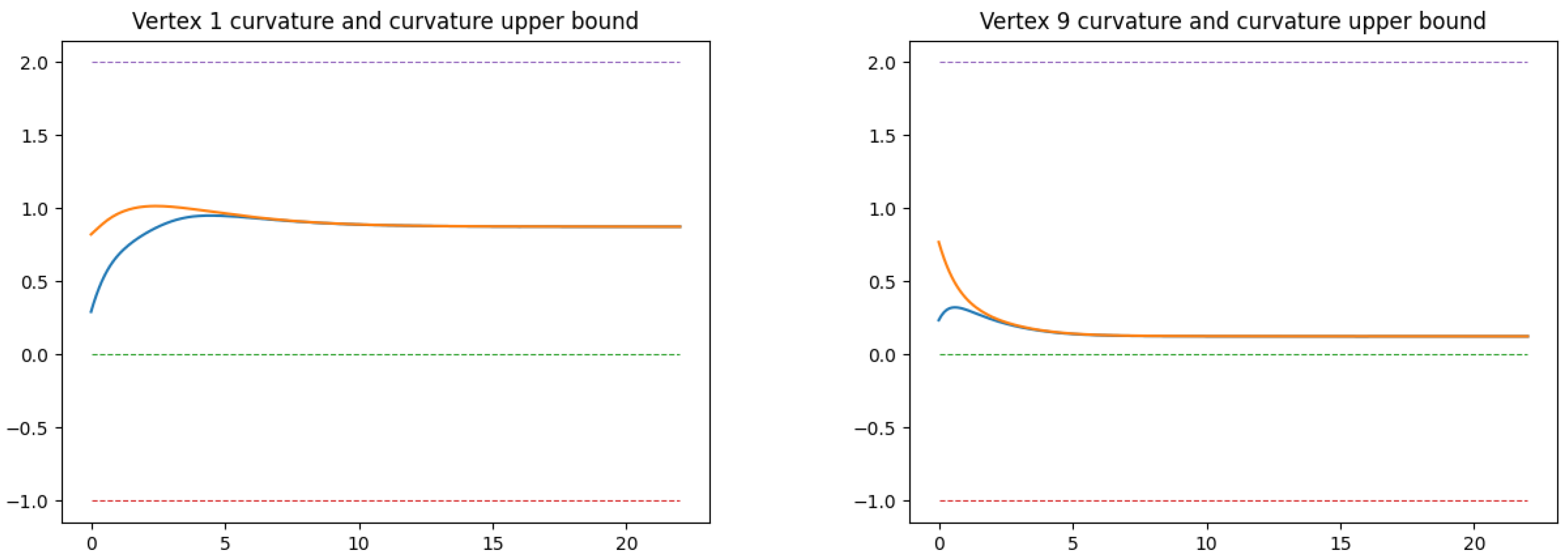
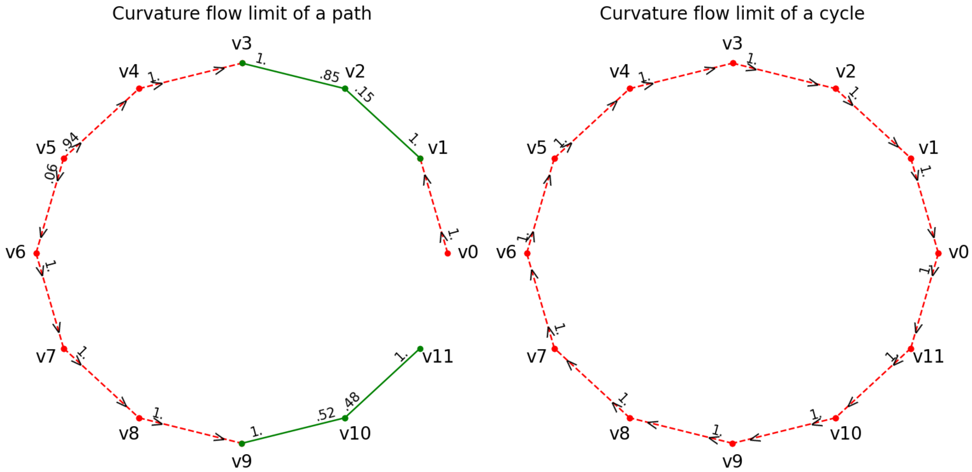
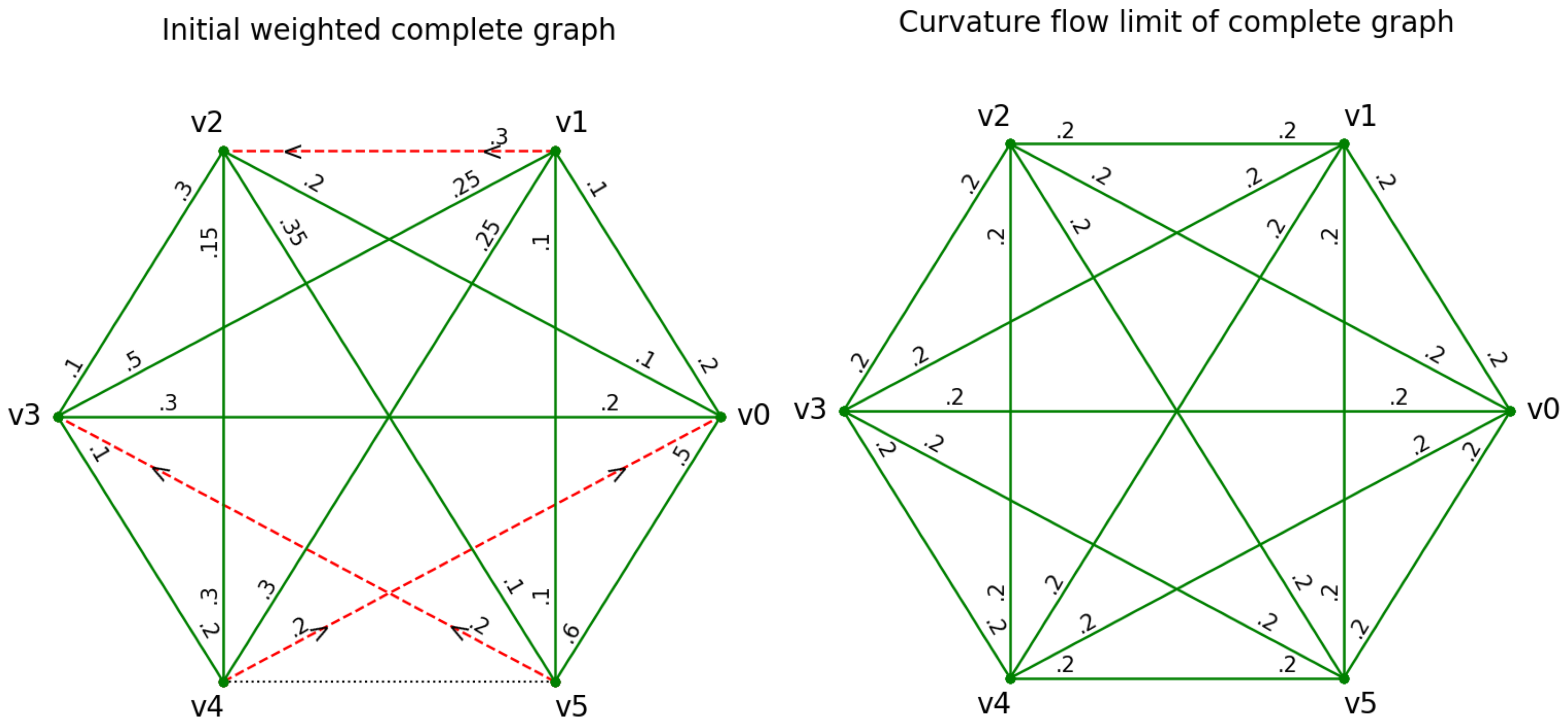
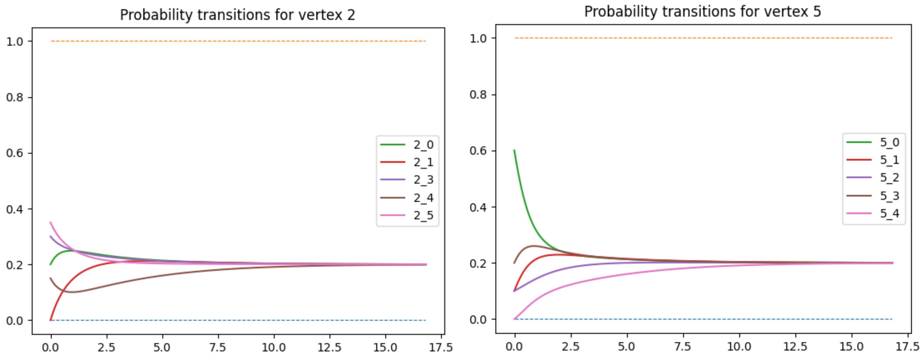
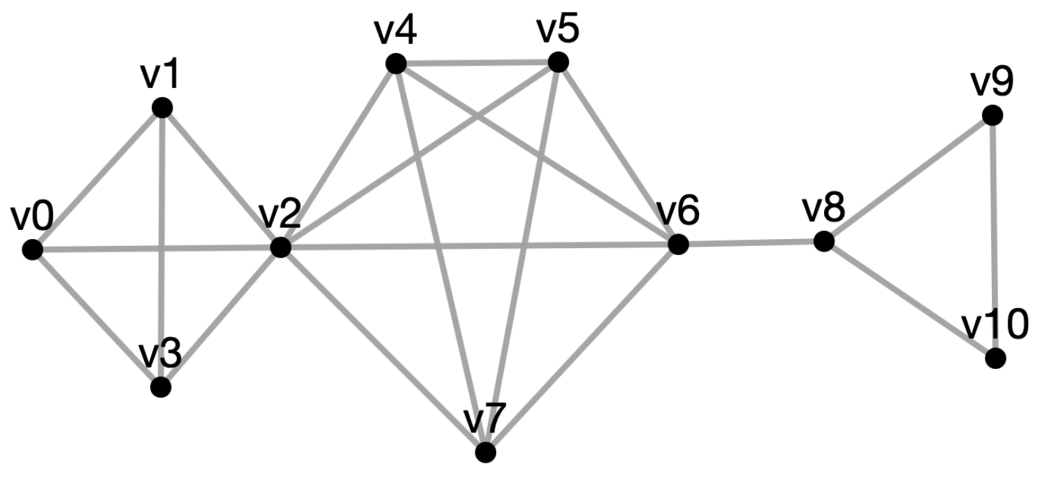
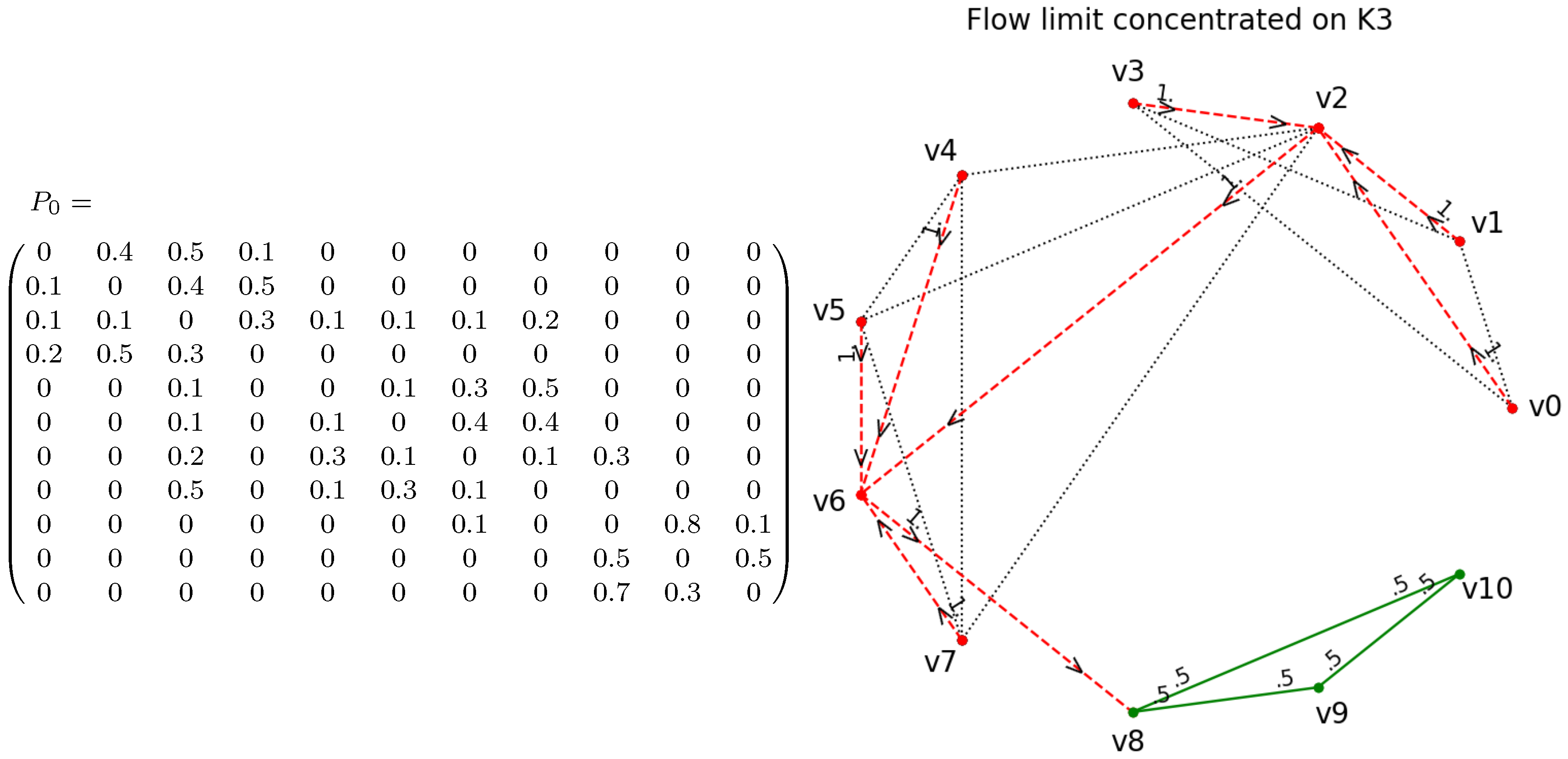
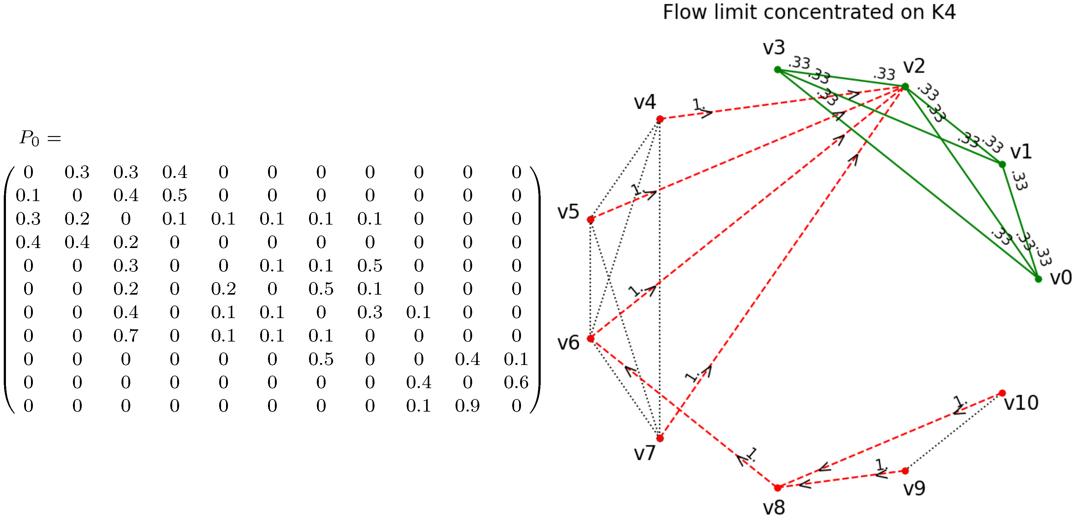
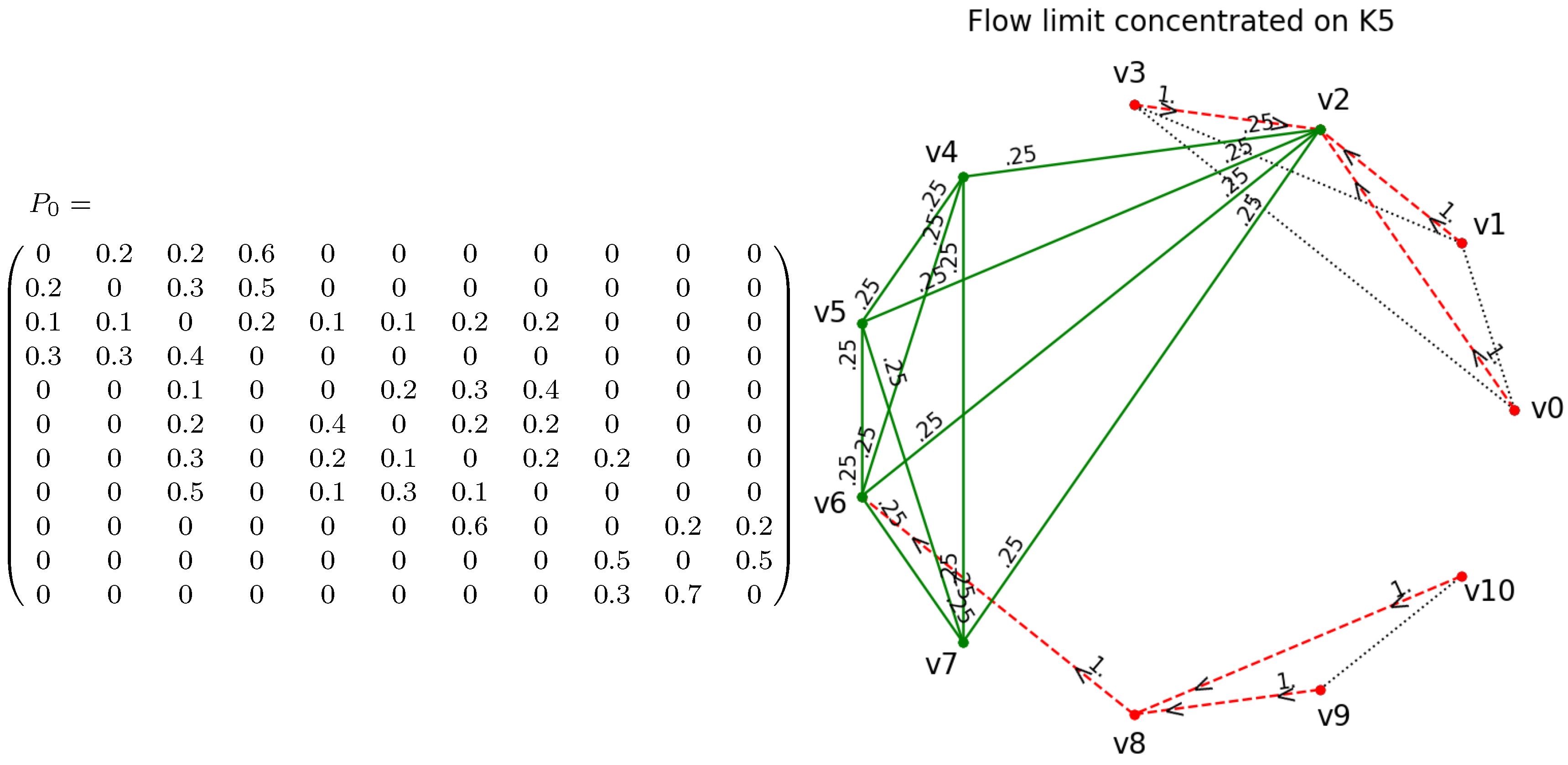
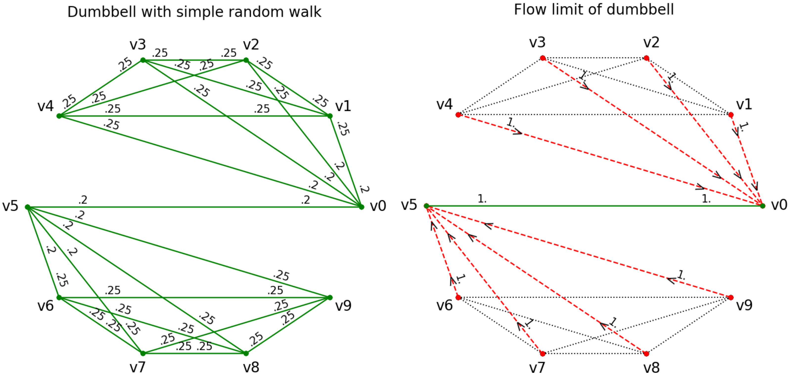
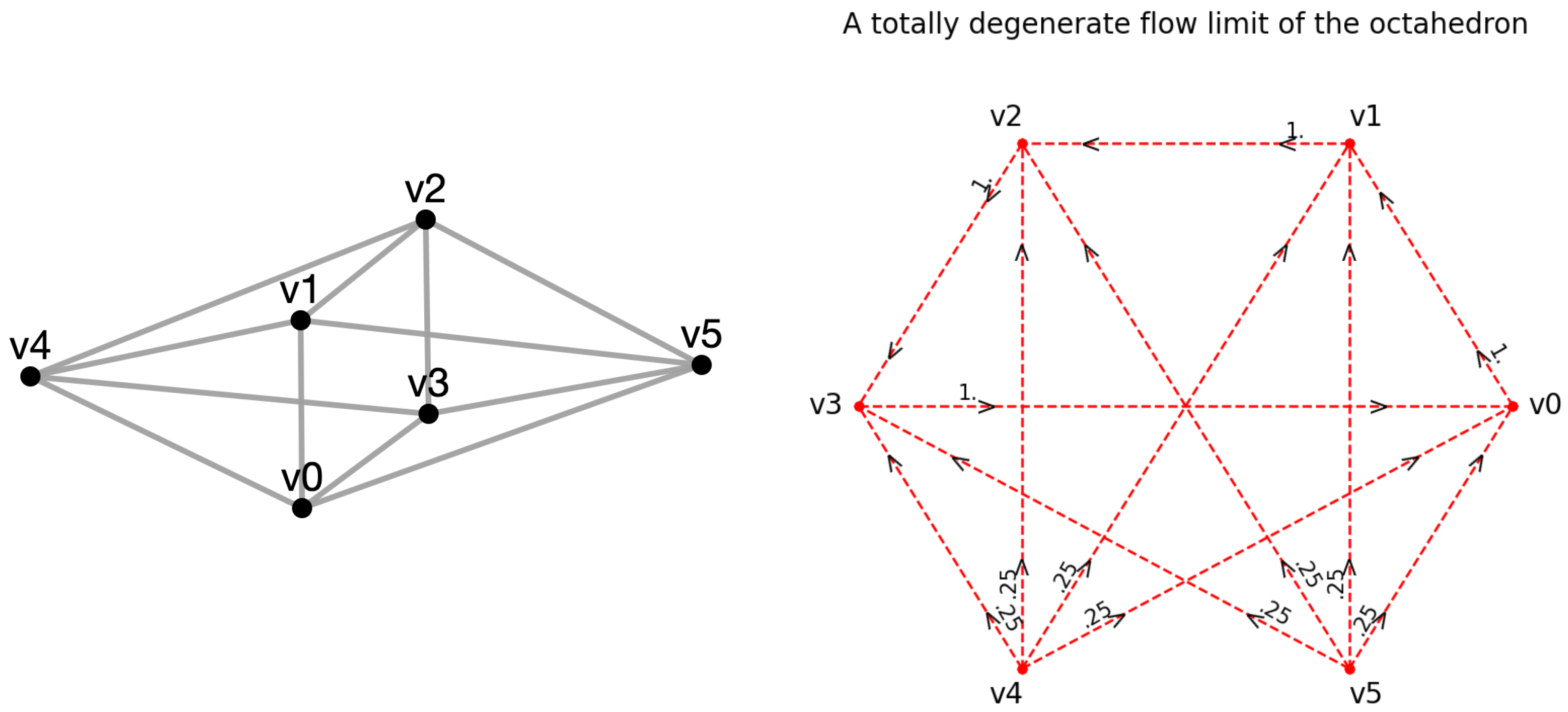
Table 1.
Vertex curvatures for the dimension ∞ of a random graph with 10 vertices at the beginning and the end of the curvature flow.
Table 1.
Vertex curvatures for the dimension ∞ of a random graph with 10 vertices at the beginning and the end of the curvature flow.
| j | ||
|---|---|---|
| 0 | ||
| 1 | ||
| 2 | ||
| 3 | ||
| 4 | 0 | |
| 5 | ||
| 6 | ||
| 7 | ||
| 8 | ||
| 9 |
Table 2.
Statistics of flow limit concentrations on the complete subgraphs and of their wedge sum, together with mean convergence times.
Table 2.
Statistics of flow limit concentrations on the complete subgraphs and of their wedge sum, together with mean convergence times.
| concentration of flow limits | ||||
| mean convergence time | – |
Disclaimer/Publisher’s Note: The statements, opinions and data contained in all publications are solely those of the individual author(s) and contributor(s) and not of MDPI and/or the editor(s). MDPI and/or the editor(s) disclaim responsibility for any injury to people or property resulting from any ideas, methods, instructions or products referred to in the content. |
© 2023 by the authors. Licensee MDPI, Basel, Switzerland. This article is an open access article distributed under the terms and conditions of the Creative Commons Attribution (CC BY) license (https://creativecommons.org/licenses/by/4.0/).
Share and Cite
MDPI and ACS Style
Cushing, D.; Kamtue, S.; Liu, S.; Münch, F.; Peyerimhoff, N.; Snodgrass, B. Bakry–Émery Curvature Sharpness and Curvature Flow in Finite Weighted Graphs: Implementation. Axioms 2023, 12, 577. https://doi.org/10.3390/axioms12060577
AMA Style
Cushing D, Kamtue S, Liu S, Münch F, Peyerimhoff N, Snodgrass B. Bakry–Émery Curvature Sharpness and Curvature Flow in Finite Weighted Graphs: Implementation. Axioms. 2023; 12(6):577. https://doi.org/10.3390/axioms12060577
Chicago/Turabian StyleCushing, David, Supanat Kamtue, Shiping Liu, Florentin Münch, Norbert Peyerimhoff, and Ben Snodgrass. 2023. "Bakry–Émery Curvature Sharpness and Curvature Flow in Finite Weighted Graphs: Implementation" Axioms 12, no. 6: 577. https://doi.org/10.3390/axioms12060577
Note that from the first issue of 2016, this journal uses article numbers instead of page numbers. See further details here.