
Matrix Representations for a Class of Eigenparameter Dependent Sturm–Liouville Problems with Discontinuity
School of Mathematical Sciences, Qufu Normal University, Qufu 273165, China
*
Author to whom correspondence should be addressed.
Axioms 2023, 12(5), 479; https://doi.org/10.3390/axioms12050479
Submission received: 18 April 2023
/
Revised: 9 May 2023
/
Accepted: 12 May 2023
/
Published: 15 May 2023
(This article belongs to the Special Issue Theory of Functions and Applications)
Abstract
:Matrix representations for a class of Sturm–Liouville problems with eigenparameters contained in the boundary and interface conditions were studied. Given any matrix eigenvalue problem of a certain type and an eigenparameter-dependent condition, a class of Sturm–Liouville problems with this specified condition was constructed. It has been proven that each Sturm–Liouville problem is equivalent to the given matrix eigenvalue problem.
1. Introduction
Recently, Sturm–Liouville problems (SLPs) with discontinuity inside intervals have attracted significant attention from scholars due to their wide application in various fields. For example, one application involves a string loaded with point masses [1,2,3,4,5]. Generally speaking, the eigenparameter only appears in the equation, but in many actual phenomena, it is necessary for the eigenparameter to appear in the boundary conditions, such as heat conduction at the liquid–solid interface [6], and so on. Due to its physical significance, many scholars have studied the problem of boundary conditions containing a spectral parameter [7,8,9,10,11,12,13,14]. In recent decades, more researchers have studied eigenparameter-dependent SLPs with discontinuity, including the asymptotic behavior of eigenvalues, the inverse spectral theory, the finite spectrum, the oscillation of eigenfunctions, etc., see [9,10,15,16,17,18,19].
Regular SLPs have an infinite countable number of eigenvalues that are bounded below and unbounded above. However, Atkinson, in his well-celebrated book [20], stated that finite eigenvalues may exist under certain conditions. Kong and Zettl [18] solved this problem by constructing a class of regular SLPs, which has exactly eigenvalues for every positive integer ; they obtained the corresponding matrix representations in [19]. This special problem is called Atkinson-type SLPs (ASLPs). Ao et al. generalized this problem to various differential operators, for example, ASLPs with interface conditions, ASLPs with eigenparameters contained in boundary conditions, higher-order differential operators, etc. [21,22,23,24,25,26]. They discussed the existence of a finite spectrum and gave the corresponding matrix representation. In particular, Ao et al. proved that ASLPs with interface conditions have, at most, eigenvalues and gave the corresponding matrix representation in [23]. Moreover, the authors generalized the problem to eigenparameter-dependent ASLPs [24].
In recent years, SLPs with interface conditions dependent on parameters have also captured the attention of researchers, see [2,3,4] and references therein. In reference [2], the author obtained the operator–theoretic formulation. The asymptotic properties of eigenvalues were given for SLPs with interface conditions that were rationally dependent on the parameters in [3]. In work by Mukhtarov et al. [4], Green’s function was provided for eigenparameter-dependent SLPs with interface conditions.
In a recent paper, Ao et al. proved that SLPs with interface conditions dependent on the eigenparameter still have a finite spectrum [27]. Here, the following question arises: When the eigenparameter appears in both the boundary and interface conditions, does it affect the number in the spectrum? In this paper, we will solve this problem. We study an SLP in which an eigenparameter is contained in both the boundary and interface conditions, regardless of whether it is self-adjoint or non-self-adjoint. We prove that the problem has, at most, eigenvalues, which is different from the results in [27], where the number of eigenvalues is, at most, . Moreover, we provide an example to illustrate our conclusion (as it turns out, it affects the number of eigenvalues). The basic method we used in this paper is a factorization of the characteristic function.
The rest of this paper is organized as follows: Some preliminaries are given in Section 2. In Section 3, we show that the number of eigenvalues of the considered problem is finite. In Section 4, the corresponding matrix representation is given, and for a given specific type of matrix eigenvalue problem, we construct a class of SLPs with the same boundary and interface conditions, ensuring that they have the same eigenvalues.
2. Preliminaries
In this work, we investigate the SL equation
with boundary conditions at the endpoints c and d, as follows
and interface conditions
where and denote the right and left limits of at , respectively. is a spectral parameter; (), and
We assume that the coefficients satisfy the following conditions
where .
Equation (1) can be represented as
by using
Let be the fundamental solution matrix of system (10), satisfying (4) and (5) as follows
with the initial condition .
Define . Let
where
By a direct calculation, we know
since , so , we have
Proof.
We suppose , then the equation has non-zero solutions. We solve the initial value problem
then we have and , we can obtain , so is an eigenvalue.
On the contrary, if is an eigenvalue and f is an eigenfunction, then satisfies ; thus, . If , then it is a trivial solution. This contradicts f being an eigenfunction, so we have . □
3. The Finite Spectrum Problem of (1)–(5)
Problems (1)–(5) have finite eigenvalues in this section. In the sequel, we always suppose that (7) holds, and there is a partition of
for , such that
Definition 2.
Definition 3.
Next, we give two fundamental solution matrices of system (10).
Lemma 1.
In general, for , we have
particularly,
Proof.
From (14), we know that u is constant on by and v is constant on by . Thus, we can obtain the result by using the iterative method. □
Using similar methods in Lemma 1, we have
Lemma 2.
For each , we denote
a fundamental solution matrix of the system (10) with interface conditions (4) and (5), and satisfy the initial condition . Then we have
Generally, for ,
Proof.
From the two fundamental solutions, and of system (10), and the given initial value, we can obtain
from (4) and (5), we have
Particularly, let , we obtain
□
In light of Lemmas 1–3, we can obtain the following theorem, and problems (1)–(5) have finite eigenvalues:
| Conditions | The number of eigenvalues |
If none of the conditions in the table above are met, then (1)–(5) have ι eigenvalues for or the system can be degenerate.
Proof.
Firstly, by Lemma 3, we know that ; next, we can obtain the structure of by a direct calculation.
If , we can obtain the structure of , as follows:
where when min , .
So if , it follows that the degrees of and in are , , , and , respectively. According to (12) and Proposition 1, if in , we can obtain the highest degree of in is ; hence, has roots. Moreover, other cases can be obtained by using similar methods.
□
Remark 1.
In Theorem 1, if , but , we can obtain the same conclusions. In fact, the highest degree of μ in is . Thus, it has , , , , eigenvalues, respectively.
Example 1.
We study a specific SLP:
where
We choose , and are piece-wise constant functions:
From the conditions, we know . By a direct calculation, we have
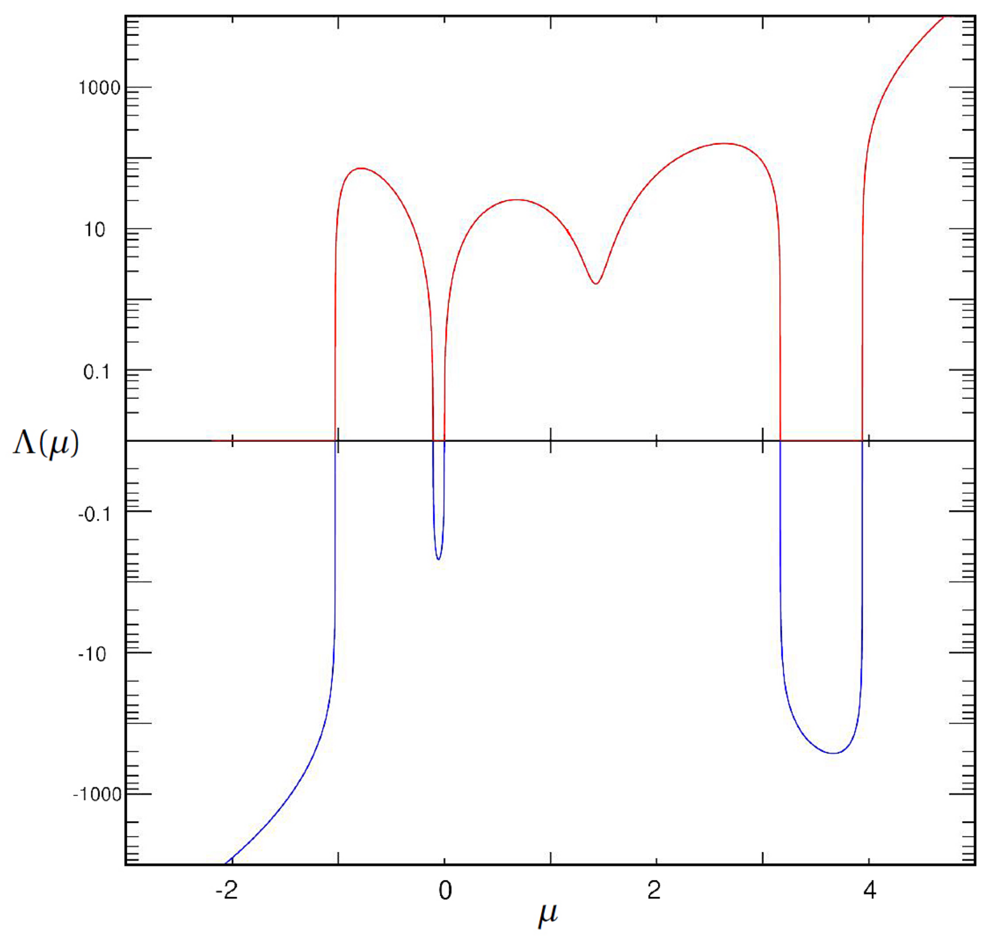
Then the number of eigenvalues of this problem is 7.
Figure 1 shows the trace of . For clarity, we use a logarithmic scale for the vertical axis. We label trajectories above the horizontal axis in red and trajectories below the horizontal axis in blue. The alternating red and blue pattern represents the zero of the . By doing so, we can observe that the function has five real roots, meeting our desired outcome.
4. Matrix Presentations of (1)–(5)
Definition 5.
If the eigenvalues of SLPs of the Atkinson type coincide with matrix eigenvalue problems, then we call them equivalent.
For (1)–(5), we rebuild the matrix eigenvalue problems, which have the following form
whose eigenvalues coincide with the corresponding SLPs of the Atkinson type. Assume (16) holds, we have
In accordance with (14) and (15), we know . In addition, by (14) and (15), for each solution of system (10), on the sub-intervals where , we know that u is constant; regarding the sub-intervals where , we know that v is constant.
Let
and
Lemma 4.
Theorem 2.
Proof.
Between the solutions of the following system:
and those of (21)–(24), a one-to-one correspondence exists by the assumption.
Now, we suppose and are solutions of systems (21) and (22). Then (26)–(28) follow from (21) to (22). Similarly, (29)–(31) follow from (23) to (24) by assuming that and are solutions of systems (23) and (24).
In other words, let be a solution of (26)–(28); thus, and can be calculated by (26) and (28). Assume that is defined in (21). Then, using (26), and utilizing induction on (27), (22) holds. Moreover, (23) and (24) can be similarly obtained.
Hence, according to Theorem 2, any solution of (10) is uniquely determined by solutions of (26)–(31). Note the first row of matrix (25)
and the last row of matrix (25)
substituting
into (32) and (33), we obtain (2) and (3). From (4) to (5), we obtain
and let Then the equivalence follows from (26) to (34). □
The following result shows that the SLP of the Atkinson type is equivalent to the SLP with piecewise constant coefficients in the sense that they have similar eigenvalues.
Theorem 3.
Proof.
In light of Theorem 3, we know that for a fixed set of Equations (2)–(5) on a given interval, there exists a family of SLPs of the Atkinson type, which have the same eigenvalues as SLPs (38), (2)–(5). We refer to this family as the equivalent family of SLPs (38), (2)–(5).
Next, we will illustrate that matrix eigenvalue problems in the following form:
have representations as Atkinson-type SLPs.
Theorem 4.
Let , in (4) and (5) satisfy (where is defined in (9)), assume . Assume that A is an matrix as follows:
where . Let F be an matrix of the following form:
where , , and
Then (39) represents an Atkinson-type SLP in the form of (1)–(5). Furthermore, SLPs (38), (2)–(5) have unique representations when a fixed partition (13) of is given, using the notations in (16) and (18). All SL representations of (39) are given by the corresponding equivalent families of SLPs (38), (2)–(5).
Proof.
For a given partition of by (13), one can define piecewise constant functions and on the interval that satisfies (7), (14) and (15), as follows:
and
Next, we define and by (35)–(37), respectively. Such piecewise constant functions, , and on interval , satisfying (7) and (14) and (15), are found; Equation (38) is of the Atkinson type, and (16) and (18) satisfy with , and w replaced by , and , respectively. Obviously, Equation (39) is of the same form as Equation (25). Therefore, the problem (39) is equivalent to the SLPs (1)–(5) by Theorem 2. The last part is yielded by Theorem 3. □
Author Contributions
Writing-original draft preparation, S.L.; writing-review and supervision, J.C.; review and editing, K.L. All authors have read and agreed to the published version of the manuscript.
Funding
This research is supported by the Natural Science Foundation of Shandong Province (nos. ZR2020QA010, ZR2020QA009), Postdoctoral Foundation of China (2020M682139), and the Natural Science Foundation of China (61973183).
Data Availability Statement
Data sharing is not applicable to this article as no datasets were generated or analyzed during the current study.
Acknowledgments
The authors thank the reviewers for their comments and detailed suggestions. They significantly improved the presentation of this paper.
Conflicts of Interest
The authors declare no conflict of interest.
References
- Likov, A.V. The Theory of Heat and Mass Transfer, 2nd ed.; Springer: Berlin/Heidelberg, Germany, 1963. (In Russian) [Google Scholar]
- Şen, E. A class of second-order differential operators with eigenparameter-dependent boundary and transmission conditions. Math. Methods Appl. Sci. 2014, 37, 2952–2961. [Google Scholar] [CrossRef]
- Bartels, C.; Currie, S.; Watson, B.A. Sturm-Liouville problems with transfer condition Herglotz-dependent on the eigenparameter: Eigenvalue asymptotics. Complex Anal. Oper. Theory 2021, 71, 1–29. [Google Scholar] [CrossRef]
- Akdoğan, Z.; Demirci, M.; Mukhtarov, O.S. Green function of discontinuous boundary value problem with transmission conditions. Math. Methods Appl. Sci. 2007, 30, 1719–1738. [Google Scholar] [CrossRef]
- Mukhtarov, O.S.; Aydemir, K. Spectral analysis of alpha-semi periodic 2-interval Sturm-Liouville problems. Qual. Theory Dyn. Syst. 2022, 21, 1–14. [Google Scholar] [CrossRef]
- Fulton, C. Two-point boundary value problems with eigenvalue parameter contained in the boundary conditions. Proc. R. Soc. Edinb. Sect. Math. 1977, 77, 293–308. [Google Scholar] [CrossRef]
- Guo, Y.; Wei, G. Inverse nodal problem for Dirac equations with boundary conditions polynomially dependent on the spectral parameter. Results Math. 2015, 67, 95–110. [Google Scholar] [CrossRef]
- Kerimov, N.B.; Maris, E.A. On the uniform convergence of Fourier series expansions for Sturm-Liouville problems with a spectral parameter in the boundary conditions. Results Math. 2018, 102, 1–16. [Google Scholar] [CrossRef]
- Sat, M. Interior inverse problem for Sturm-Liouville operator with eigenparameter dependent boundary conditions. In Bulletin of the Transilvania; Series III: Mathematics, Informatics, Physics; University of Brasov: Brasov, Romania, 2017; Volume 10, pp. 129–141. [Google Scholar]
- Yang, C.; Pivovarchik, V.N. Inverse nodal problem for Dirac system with spectral parameter in boundary conditions. Complex Anal. Oper. Theory 2013, 7, 1211–1230. [Google Scholar] [CrossRef]
- Li, K.; Zhang, M.; Zheng, Z. Dependence of eigenvalues of Dirac system on the parameters. Stud. Appl. Math. 2023, 150, 1201–1216. [Google Scholar] [CrossRef]
- Guliyev, N.J. Schrödinger operators with distributional potentials and boundary conditions dependent on the eigenvalue parameter. J. Math. Phys. 2019, 60, 063501. [Google Scholar] [CrossRef]
- Guliyev, N.J. A Riesz basis criterion for Schrödinger operators with boundary conditions dependent on the eigenvalue parameter. Anal. Math. Phys. 2020, 60, 1–8. [Google Scholar] [CrossRef]
- Guliyev, N.J. On two-spectra inverse problems. Proc. Amer. Math. Soc. 2020, 10, 4491–4502. [Google Scholar] [CrossRef]
- Yang, C.; Yang, X. An interior inverse problem for the Sturm-Liouville operator with discontinuous conditions. Appl. Math. Lett. 2009, 22, 1315–1319. [Google Scholar] [CrossRef]
- Prather, C.L.; Shaw, J.K. On the oscillation of differential transforms of eigenfunction expansions. Trans. Am. Math. Soc. 1983, 280, 187–206. [Google Scholar] [CrossRef]
- Zhang, L.; Ao, J. Inverse spectral problem for Sturm-Liouville operator with coupled eigenparameter dependent boundary conditions of the Atkinson type. Inverse Probl. Sci. Eng. 2019, 27, 1689–1702. [Google Scholar] [CrossRef]
- Kong, Q.; Wu, H.; Zettl, A. Sturm-Liouville problems with finite spectrum. J. Math. Anal. Appl. 2001, 263, 748–762. [Google Scholar] [CrossRef]
- Kong, Q.; Volkmer, H.; Zettl, A. Matrix representations of Sturm-Liouville problems with finite spectrum. Results Math. 2009, 54, 103–116. [Google Scholar] [CrossRef]
- Atkinson, F.V. Discrete and Continuous Boundary Value Problems, 2nd ed.; Academic Press: New York, NY, USA; London, UK, 1964. [Google Scholar]
- Ao, J.; Sun, J. Matrix representations of fourth-order boundary value problems with coupled or mixed boundary conditions. Linear Multilinear Algebra 2015, 63, 1590–1598. [Google Scholar] [CrossRef]
- Ao, J.; Sun, J.; Zhang, M. The finite spectrum of Sturm-Liouville problems with transmission conditions. Appl. Math. Comput. 2011, 218, 1166–1173. [Google Scholar] [CrossRef]
- Ao, J.; Sun, J.; Zhang, M. Matrix representations of Sturm-Liouville problems with transmission conditions. Comput. Math. Appl. 2012, 63, 1335–1348. [Google Scholar] [CrossRef]
- Ao, J.; Sun, J.; Zhang, M. The finite spectrum of Sturm-Liouville problems with transmission conditions and eigenparameter dependent boundary conditions. Results Math. 2013, 63, 1057–1070. [Google Scholar] [CrossRef]
- Ge, S.; Wang, W.; Ao, J. Matrix representations of fourth order boundary value problems with periodic boundary conditions. Appl. Math. Comput. 2014, 227, 601–609. [Google Scholar] [CrossRef]
- Cai, J.; Zheng, Z. Matrix representations of Sturm-Liouville problems with coupled eigenparameter dependent boundary conditions and transmission conditions. Math. Methods Appl. Sci. 2018, 41, 3495–3508. [Google Scholar] [CrossRef]
- Zhang, N.; Ao, J.-J. Finite spectrum of Sturm-Liouville problems with transmission conditions dependent on the spectral parameter. Numer. Funct. Anal. Optim. 2023, 44, 21–35. [Google Scholar] [CrossRef]
Figure 1.
Characteristic function in Example 1.

Disclaimer/Publisher’s Note: The statements, opinions and data contained in all publications are solely those of the individual author(s) and contributor(s) and not of MDPI and/or the editor(s). MDPI and/or the editor(s) disclaim responsibility for any injury to people or property resulting from any ideas, methods, instructions or products referred to in the content. |
© 2023 by the authors. Licensee MDPI, Basel, Switzerland. This article is an open access article distributed under the terms and conditions of the Creative Commons Attribution (CC BY) license (https://creativecommons.org/licenses/by/4.0/).
Share and Cite
MDPI and ACS Style
Li, S.; Cai, J.; Li, K. Matrix Representations for a Class of Eigenparameter Dependent Sturm–Liouville Problems with Discontinuity. Axioms 2023, 12, 479. https://doi.org/10.3390/axioms12050479
AMA Style
Li S, Cai J, Li K. Matrix Representations for a Class of Eigenparameter Dependent Sturm–Liouville Problems with Discontinuity. Axioms. 2023; 12(5):479. https://doi.org/10.3390/axioms12050479
Chicago/Turabian StyleLi, Shuang, Jinming Cai, and Kun Li. 2023. "Matrix Representations for a Class of Eigenparameter Dependent Sturm–Liouville Problems with Discontinuity" Axioms 12, no. 5: 479. https://doi.org/10.3390/axioms12050479
Note that from the first issue of 2016, this journal uses article numbers instead of page numbers. See further details here.