
Parametric Expansions of an Algebraic Variety near Its Singularities

1
Keldysh Institute of Applied Mathematics of RAS, 125047 Moscow, Russia
2
Department of Algebra and Geometry, Samarkand State University Named after Sh. Rashidov, Samarkand 140104, Uzbekistan
*
Author to whom correspondence should be addressed.
†
These authors contributed equally to this work.
Axioms 2023, 12(5), 469; https://doi.org/10.3390/axioms12050469
Submission received: 26 December 2022
/
Revised: 25 April 2023
/
Accepted: 9 May 2023
/
Published: 13 May 2023
(This article belongs to the Special Issue Advances in Applied Algebra, Combinatorics and Computation)
Abstract
:Presently, there is a method based on Power Geometry that allows one to find asymptotic forms and asymptotic expansions of solutions to different kinds of non-linear equations near their singularities. The method contains three algorithms: (1) Reducing the equation to its normal form, (2) separating truncated equations, and (3) power transformations of coordinates. Here, we describe the method for the simplest case, a single algebraic equation, and apply it to an algebraic variety, as described by an algebraic equation of order 12 in three variables. The variety was considered in study of Einstein’s metrics and has several singular points and singular curves. Near some of them, we compute a local parametric expansion of the variety.
1. Introduction
Here, we propose a new method for the solution of a polynomial equation
near its singular point. In this example, we demonstrate computations of the method for a certain polynomial, f and .
This method is used:
- I.
- The Newton polyhedron for separation of truncated equations and
- II.
- Power transformations for the simplification of these equations.
Below, we provide a short history of both of these objects.
I. The Newton polyhedron. For , in approximately 1670, Newton [1] suggested to use one edge of the “Newton open polygon” [2] (Part I, Ch. I, § 2) of a polynomial to find the branches of solutions to the equation , in the form
with rational power exponents p near the origin , where the polynomial f has no constant and linear terms. Puiseux [3] was already using all the edges of the Newton open polygon and had given a rigorous substantiation to the solution of the problem by this method. Liouville [4] was using this approach to find the rational solutions to the linear ordinary differential equation
where are polynomials. Briot and Bouquet [5] were using an analog to the Newton open polygon to find solutions to the nonlinear ordinary differential equation near the point , where polynomials f and g vanish. A survey of other applications of the Newton (open) polygon was made by Chebotarev [6].
Some properties of solutions in the form of expansions (2) were studied in [7]. In ([2] Part I, Chapter I, § 2, Section 2.9), a method was proposed for computing the second type of solutions to equation , in the form
where and are integral numbers and is a parameter. It must use continued fractions and power transformations.
For , in 1962, the Newton polyhedron was introduced in [8] for an autonomous system of the ordinary differential equation (ODE) and was called a polyhedron . It was used in [9,10] to study solutions to the Equation (1), in the form
where is a power series in a rational exponent of its arguments. Moreover, in [10], supports of the series in (4) belong to some cones. Such expansions were considered in [2] (Part I, Chapter I, § 3). However, not all solutions to Equation (1) have the form (4). Here, we consider solutions of the form
where coefficients are rational functions of global parameters and power exponents p of the small parameter are integers.
II. The power transformation was used by Newton [1] and all his followers in the simplest form of . Weierstrass [11] suggested the sequence of transformations and were analogous to the -process in Algebraic Geometry. Power transformations in the general form of were suggested in [8]. Hironaka [12] proved the resolution of singularities of any algebraic variety by means of a -process. However, power transformations make that happen more quickly (see [2] (Part I, Chapter I, § 2, Section 2.10)).
Here, the basic ideas of this method are explained for the simplest case: a single algebraic equation. In Section 2, we provide a generalization of the Implicit Function Theorem. In Section 3 and Section 4, we provide some constructions of Power Geometry [13]. In Section 5, we explain a way of the computation of asymptotic parametric expansions of solutions. In Section 6, we demonstrate the computation of an example in detail.
2. The Implicit Function Theorem
Let , , then
Theorem 1.
Let
where , , the sum is finite and are some functions of , besides , . Then, the solution to the equation has the form
where , , the coefficients are functions on T that are polynomials from with divided by . The expansion (6) is unique.
This is a generalization of Theorem 1.1 of [13] (Ch. II) on the implicit function and simultaneously a theorem on reducing the algebraic Equation (5) to its normal form (6) when the linear part is non-degenerate. In it, we must exclude the values of T near the zeros of the function .
Let or , and be a polynomial. A point , is called simple if the vector in it is non-zero. Otherwise, the point is called singular or critical. By shifting , we move the point to the origin . If at this point the derivative , then near all solutions to the equation have the form , that is, they lie in the -dimensional space.
3. The Newton Polyhedron
Let the point be singular. Write the polynomial in the form
where , or . Let .
The set is called the support of the polynomial . Let it consist of points . The convex hull of the support is the set
which is called the Newton polyhedron.
Its boundary consists of generalized faces of , where d is its dimension of and j is its number. The numbering is unique for all dimensions d.
Each (generalized) face corresponds to its:
- Boundary subset:
- Truncated polynomial:
- Normal: cone:where , the space is conjugate (dual) to the space and is the scalar product.
At , solutions to the full equation tend to non-trivial solutions of those truncated equations , whose normal cone intersects with the negative orthant in .
4. Power Transformations
Let . The linear transformation of the logarithms of the coordinates is
where , a nondegenerate square n-matrix, is called a power transformation.
In the power transformation (7), the monomial transforms into the monomial , where , and the asterisk indicates a transposition.
A matrix is called unimodular if all its elements are integers and . For an unimodular matrix , its inverse and transpose are also unimodular.
Theorem 2.
For the face , there exists a power transformation (7) with the unimodular matrix α which reduces the truncated sum to the sum from d coordinates, that is, , where is a polynomial. Here, . The additional coordinates are local (small).
The article [14] specifies an algorithm for computing the unimodular matrix of Theorem 2.
5. Parametric Expansion of Solutions
Let be a face of the Newton polyhedron . Let the full equation be changed into the equation after the power transformation of Theorem 2. Thus, .
Let the polynomial be the product of several irreducible polynomials
where . Let the polynomial be one of them. Three cases are possible:
Case 1. The equation has a polynomial solution . Then, in the full polynomial , let us substitute the coordinates
for the resulting polynomial , and again construct the Newton polyhedron, separate the truncated polynomials, etc. Such calculations were provided in the Introduction to [13].
Case 2. The equation has no polynomial solution, but has a parametrization of solutions
Then, in the full polynomial , we substitute the coordinates
where , , and from the full polynomial , we obtain the polynomial
where , , . Thus, , .
If in the expansion (8) , then . By Theorem 1, all solutions to the equation have the form
i.e., according to (9), the solutions to the equation have the form
Such calculations were proposed in [15] and will be shown in the following example.
If in (8) , then in (10) and for the polynomial (10) from , we construct the Newton polyhedron by supporting , separating the truncations, and so on.
Case 3. The equation has neither a polynomial solution nor a parametric one. Then, using Hadamard’s polyhedron [15], one can compute a piecewise approximate parametric solution to the equation and look for an approximate parametric expansion.
Similarly, one can study the position of an algebraic manifold in infinity.
A more conventional approach is given in [16].
6. Variety and Its Singularities
In [17,18,19,20,21,22,23,24], the investigation of the three-parametric family of special homogeneous spaces from the viewpoint of the normalized Ricci flow was started. The Ricci flows describe the evolution of Einstein’s metrics on a variety. The equations of the normalized Ricci flow are reduced to a system of two differential equations with three parameters: , and :
here, and are certain functions.
The singular point of this system are associated with the invariant Einstein’s metrics. At the singular (stationary) point , , system (11) has two eigenvalues, and . If at least one of them is equal to zero, then the singular (fixed) point , is said to be degenerate. It was proved in [17,18,19,20,21,22,23,24] that the set of the values of the parameters , , , in which system (11) has at least one degenerate singular point, is described by the equation
where , , are elementary symmetric polynomials, equal, respectively, to
In [25], for symmetry reasons, the coordinates were changed to the coordinates by the linear transformation
Definition 1.
Let be some polynomial, . A point of the set is called the singular point of the k-order, if all partial derivatives of the polynomial for the turn into zero at this point, up to and including the k-th order derivatives, and at least one partial derivative of order is nonzero.
In [25], all singular points of the variety in coordinates were found. The five points of the third order are:
| Name | Coordinates |
three points of the second order
| Name | Coordinates |
and three more algebraic curves of singular points of the first order:
The points , and are of the same type; they pass into each other when rotated in the plane by an angle , just as all points , , . The curves , , correspond to two more curves of the same type. Therefore, it is sufficient to study the variety in the neighborhood of points , , , and curves , and . In Section 7, Section 8, Section 9 and Section 10, the neighborhoods of points , , line and point are studied, correspondingly. The methods proposed in [15] and described in Section 2, Section 3, Section 4 and Section 5 are implemented.
In coordinates , the variety is described by a very cumbersome polynomial of degree 12 with rational coefficients, because the transformation from to has rational coefficients.
In the paper [26], three variants of the global parametrization of the variety were proposed. These parametrizations were computed using the parametric description of the discriminant set of a monic cubic polynomial [27] and can be written in radical form [28]. Such a global description of the variety cannot provide an adequate picture of the structure in the vicinity of its singular points.
7. The Structure of the Variety near the Singular Point
Near the point , let us introduce the local coordinates :
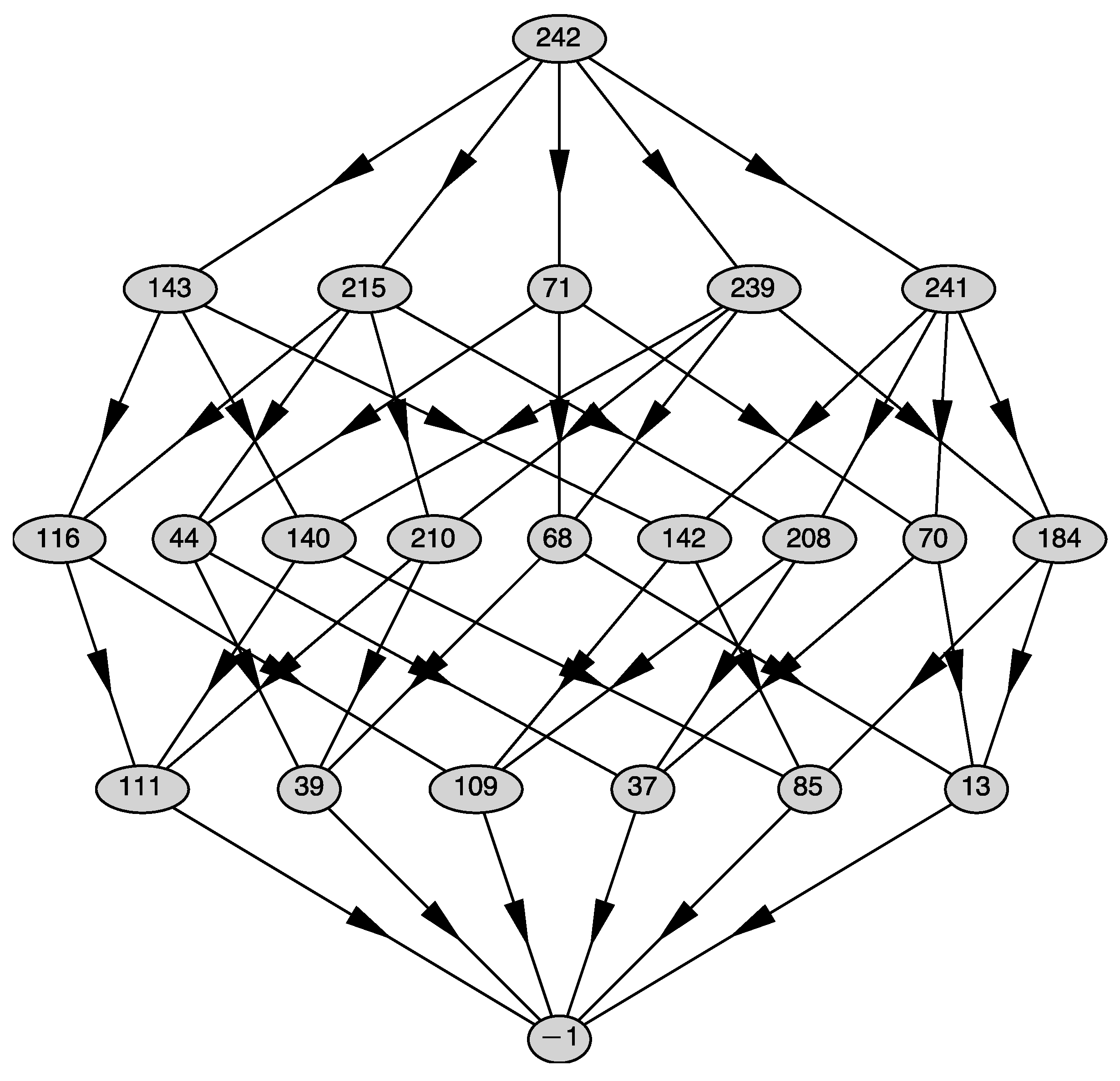
and from the polynomial , we obtain a polynomial of degree 12 . We calculate its support, the Newton polyhedron , and its faces and their external normals, using the PolyhedralSets package of the Maple 2021 computer algebra system [29]. We obtain five faces of . The graph of the polyhedron is shown in Figure 1.
Each generalized face of is presented by its number j in an oval. Numbers j are given by the program automatically. The top line of Figure 1 contains the whole polyhedron ; the next line contains all the two-dimensional faces .
Below that are the edges of , then the vertices of , and at the bottom, the empty set.
A face is connected with a face by an arrow, iff .
The external normals to its two-dimensional faces are
The neighborhood of the point is approximately described by the truncated equation
corresponding to the face of of number with the normal , which has all negative coordinates.
According to the article [14], we find the unimodular matrix such that . Consequently, we have to conduct the power transformation , i.e., .
Since , then
Here, ;
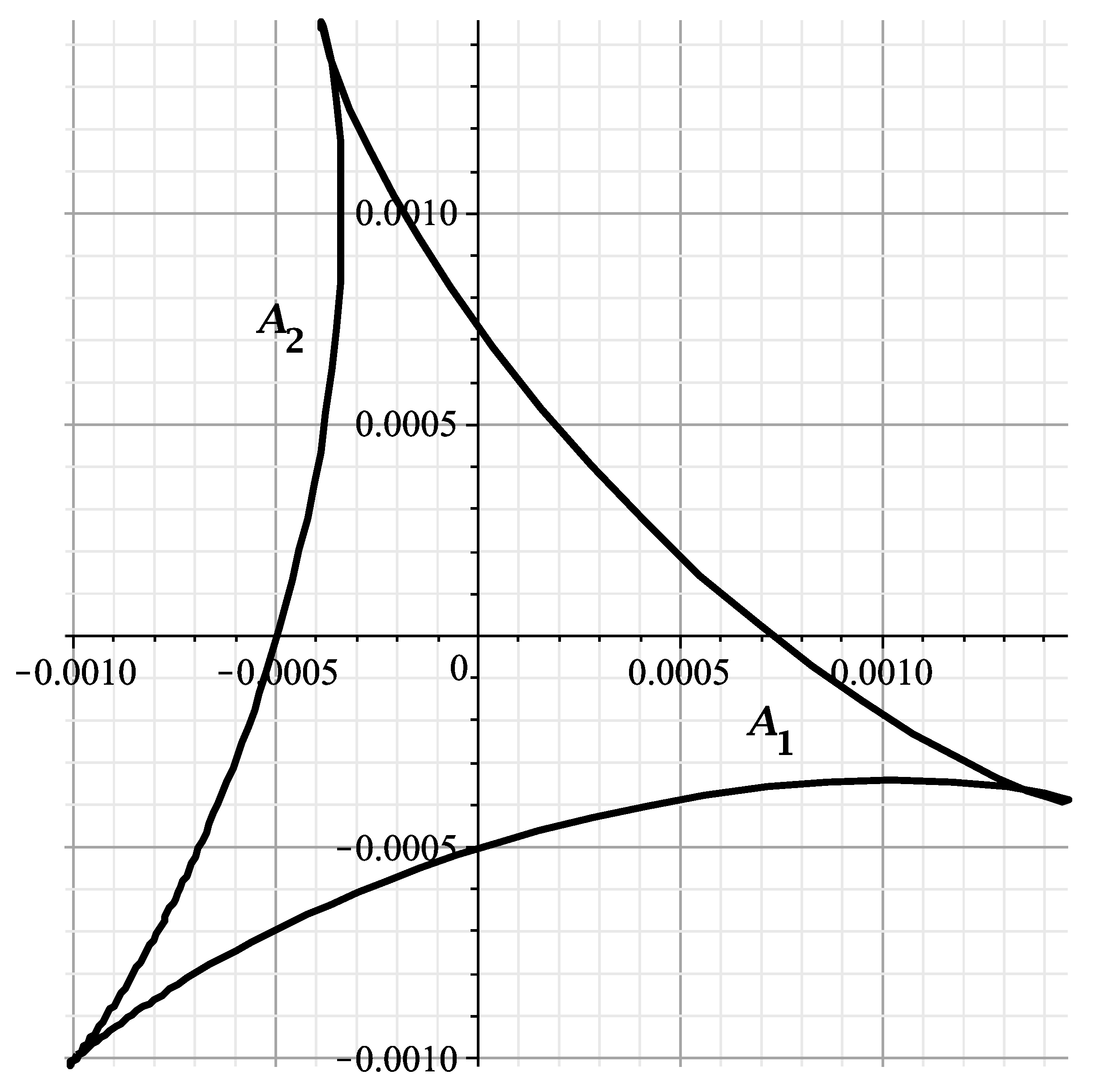
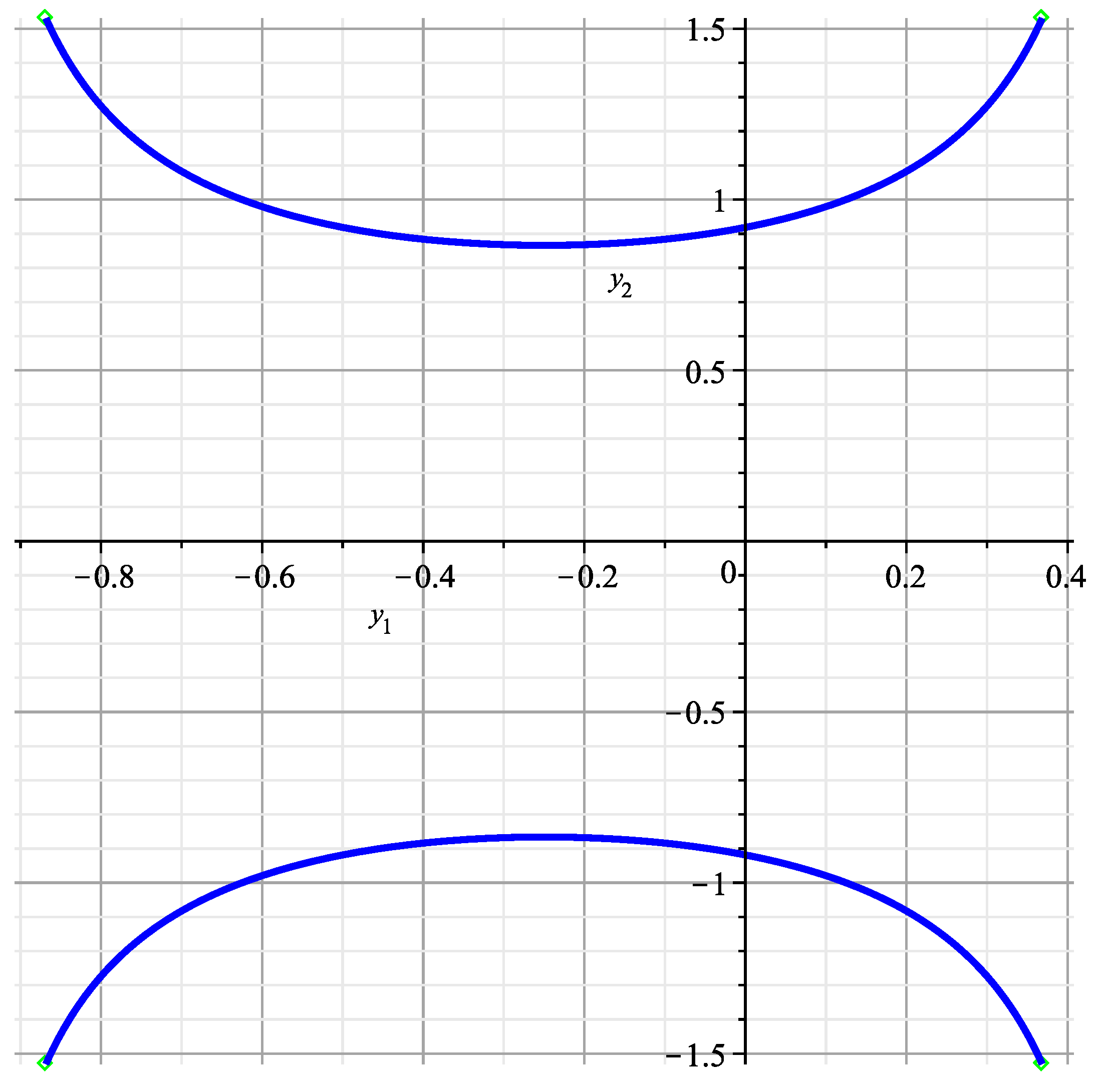
According to the algcurves package from the computer algebra system Maple, the curve has genus 0, with parametrization
and the plot shown in Figure 2.
This is a curvilinear triangle with vertices
Now, to describe the structure of the variety near the point , we substitute the power transformation (12) into the polynomial and obtain the polynomial . It decomposes into the sum
with and using the command coeff(f,x[k],m) in CAS Maple, selecting monomials containing the factor ; for and , we obtain
In the polynomials , we conduct the substitution
and obtain a polynomial with coefficients depending on t through and . In this polynomial
where of (13), so ,
and in general
when , , , according to (14) and in the substitution of (16).
The functions and each have three multiple roots
The values correspond to the vertices of the curvilinear triangle of Figure 4.
According to Theorem 1 on the implicit function, the equation has the solution as the power series over
where are rational functions that are expressed via the coefficients , which in turn are expressed via and according to (18). This decomposition is valid for all values of t, except maybe the roots in (19). In particular,
where the denominator has no real roots. According to (20), approximate .
Let us return to the initial coordinates, which for small on variety are approximated by
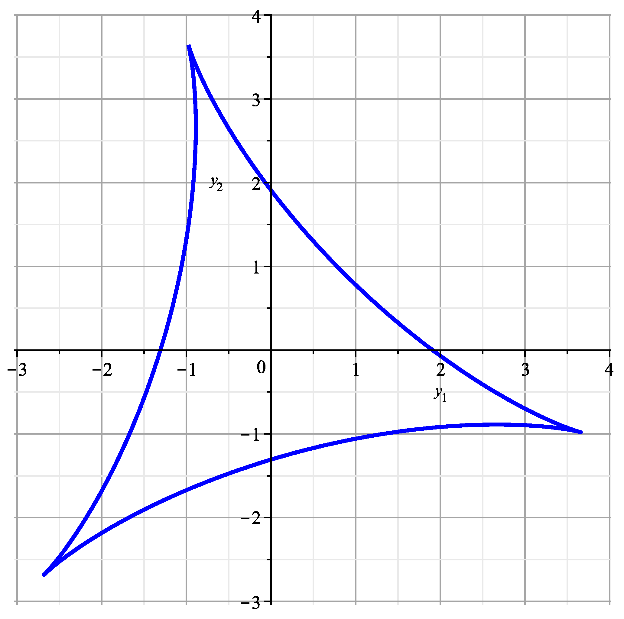
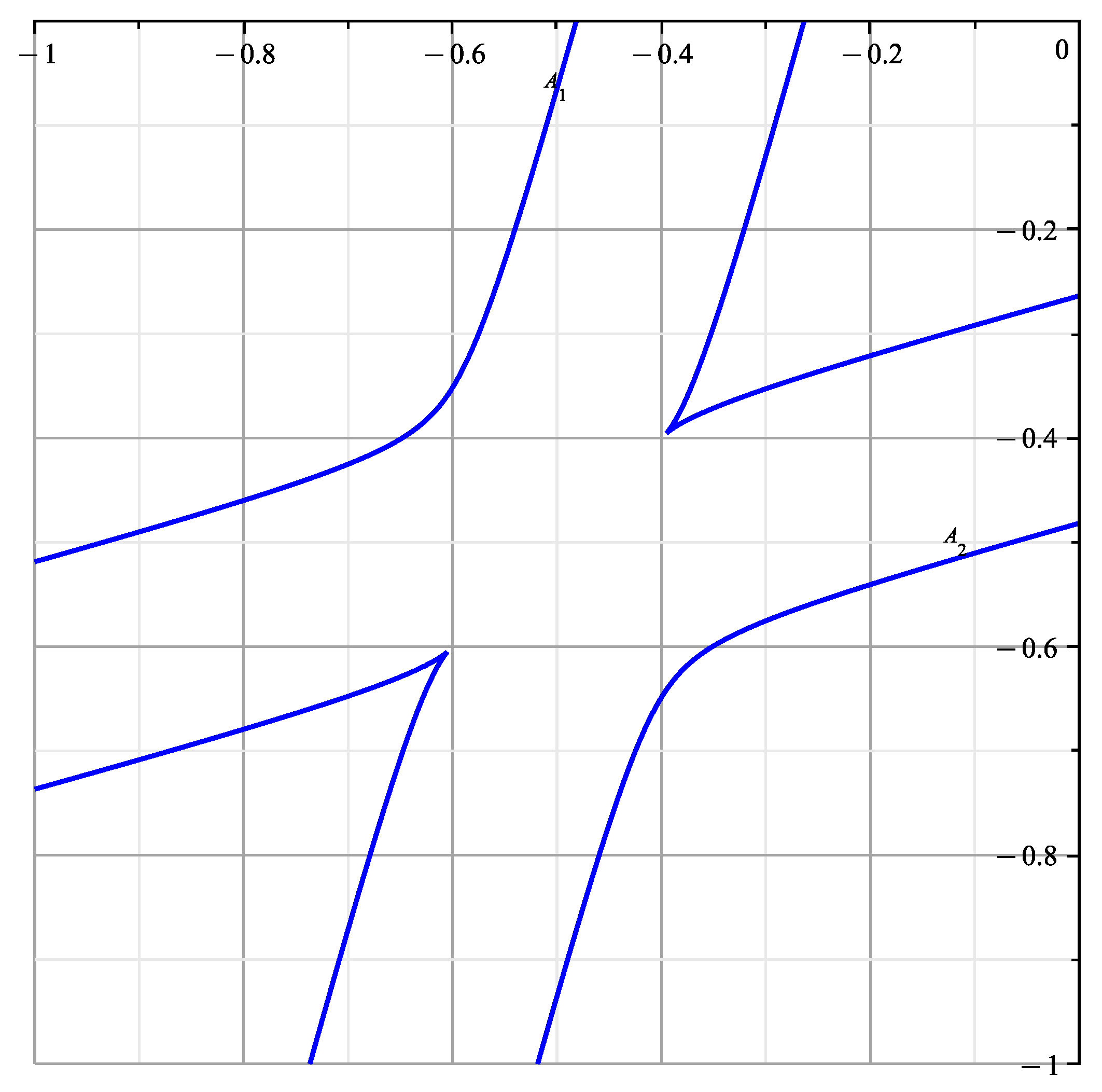
If , i.e., , the curve (21) is shown in Figure 3.
It is similar to the curve of Figure 11 in [25], with near the origin.
8. The Structure of the Variety near the Singular Point
Near the point , we introduce the local coordinates
and from the polynomial , we obtain a polynomial of degree 12
We compute its support, the Newton polyhedron , its faces and their external normals using the package PolyhedralSets of the Computer Algebra System (CAS) Maple 2021 [29]. We obtain five faces of . The graph of the polyhedron is shown in Figure 5.
The external normals of its two-dimensional faces are , , , , .
The neighborhood of point is approximately described by zeros of the truncated polynomial
corresponding to face 71 with normal which has all negative coordinates. According to the article [14], we find the unimodular matrix
such that
Hence, we have to perform the power transformation
i.e.,
Since , then
Here
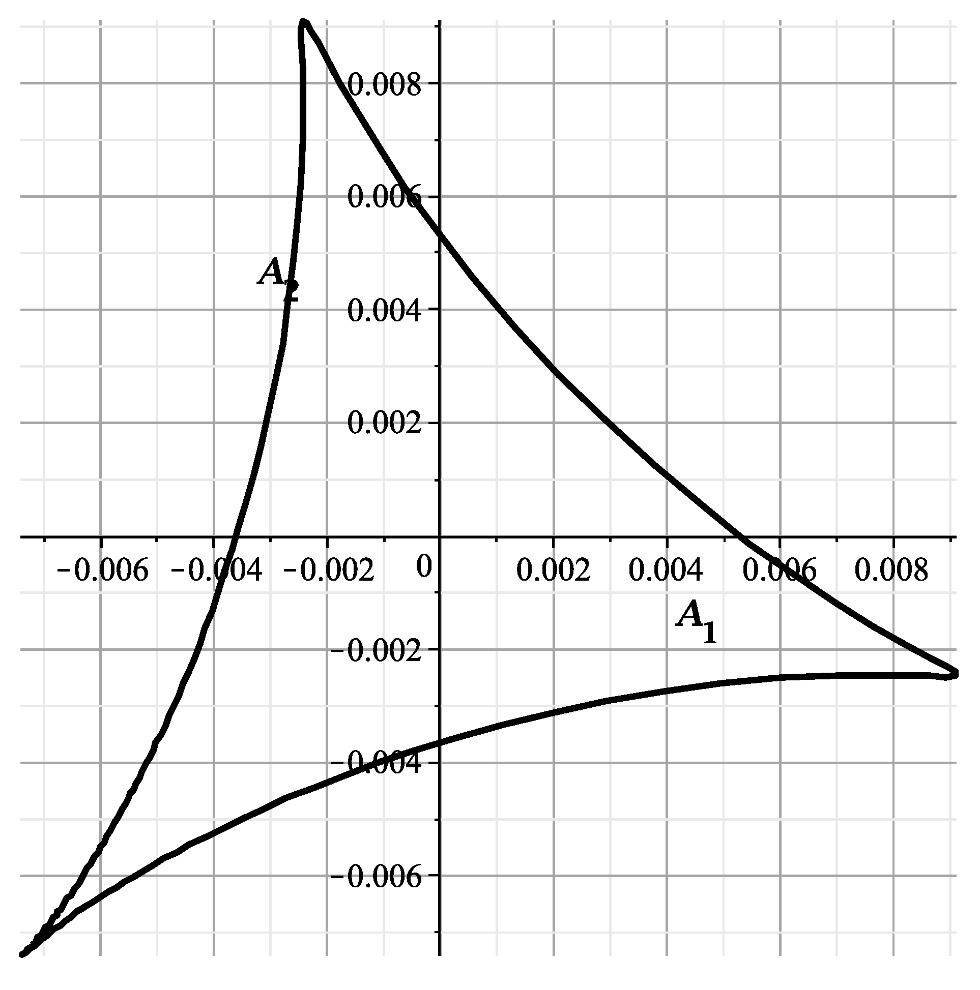
According to procedure genus from the package algcurves of the CAS Maple, the curve has genus 0, with parametrization
and the graph shown in Figure 6.
This is a curved triangle with vertices
Now, to describe the structure of the variety near the point , we substitute (24) into the polynomial and obtain the polynomial . It is divided into the sum
with , and using Maple’s command coeff, we find
In the polynomials , we conduct the substitution
We obtain a polynomial with coefficients depending on t through and In this polynomial,
where of (8); thus, ,
and in general
according to the (29) replacement. Presently, according to (28) and (30)
The functions and have three multiple roots each
In addition, has three more multiple roots
The values correspond to the vertices (27) of the curved triangle of Figure 6.
By Theorem 1, on the implicit function, the equation has a solution as a power series on
where are rational functions that are expressed over the coefficients , which in turn are expressed over and according to (31). This decomposition holds for all values of except, perhaps, the roots of (32). In particular,
where the denominator has no real roots. According to (33), we obtain the approximation of .
Let us return to the original coordinates, which for small on the variety are approximately equal
in this case
If , i.e., , then the curve (34) is shown in Figure 7. It is similar to the curve of Figure 2 in [25] near the origin, corresponding to . If , it is shown in Figure 8 and is similar to the curve of Figure 4 in [25] near the origin, corresponding to .
The similarity of these curves confirms the correctness of the found parameterization, which can be refined.
9. The Structure of the Variety near the Curve of Singular Points
On the curve and near it, let us introduce the local coordinates
On the line , the coordinates and are arbitrary.
From the polynomial , we obtain a polynomial of degree 12
we compute its support, the Newton polyhedron , its faces and their external normals, using the PolyhedralSets package of the CAS Maple 2021 [29]. We obtain seven faces . The graph of the polyhedron is shown in Figure 9.
The external normals of its two-dimensional faces are , , , , , , .
The neighborhood of the line is approximately described by the zeros of the truncated polynomial
corresponding to face 641 with normal , which has two negative coordinates. According to the paper [14], we find the unimodular matrix
such that
Hence, we have to perform the power transformation
i.e.,
Since , then
In this case
The equation has three solutions:
- . It corresponds to the point , which we will study separately in Section 10.
- . It corresponds to points and , which we will study separately.
- Curve
According to the procedure genus from the package algcurves program from the CAS Maple, the curve has a genus 0, parameterization
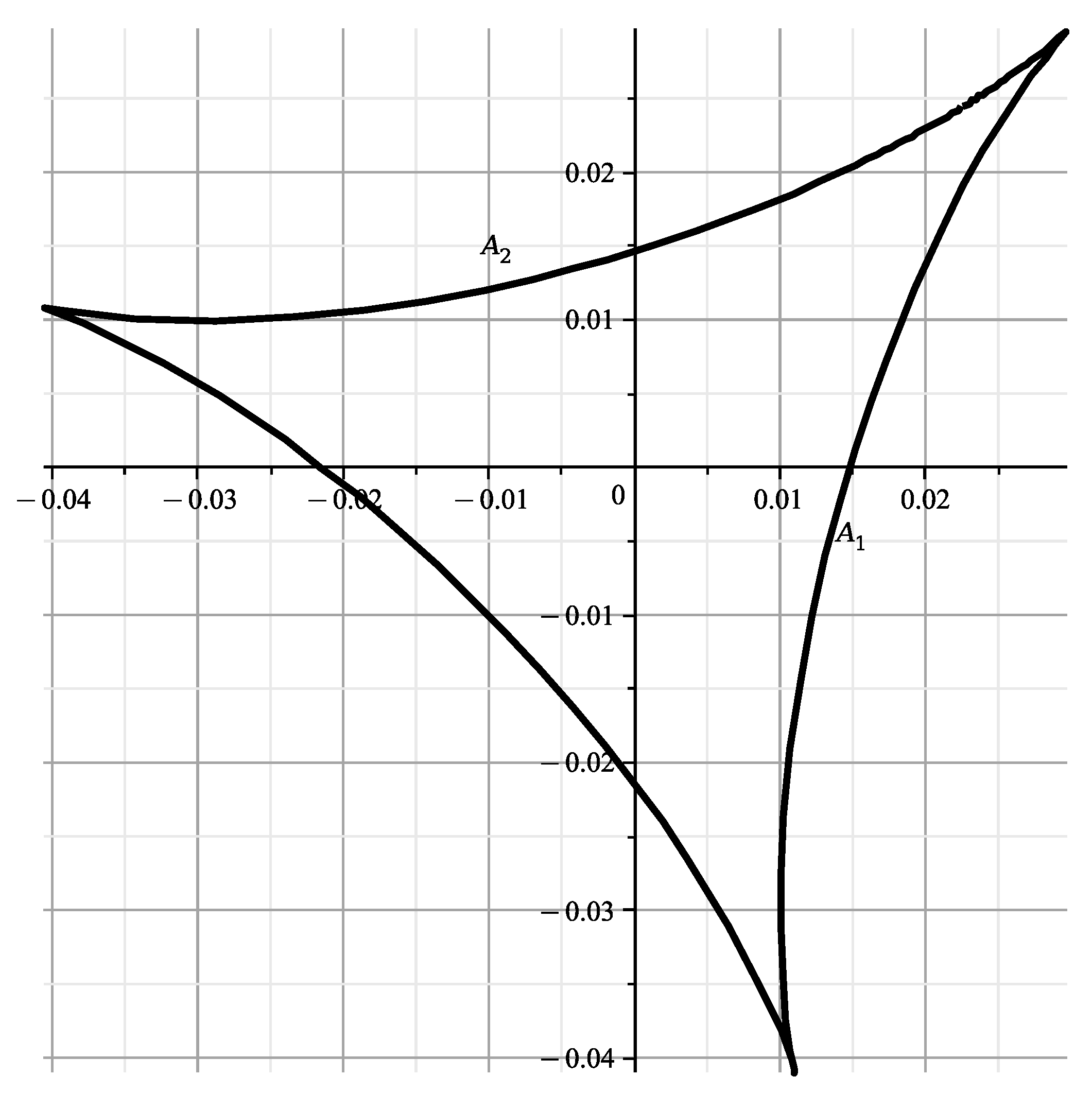
as shown in the graph in Figure 10.
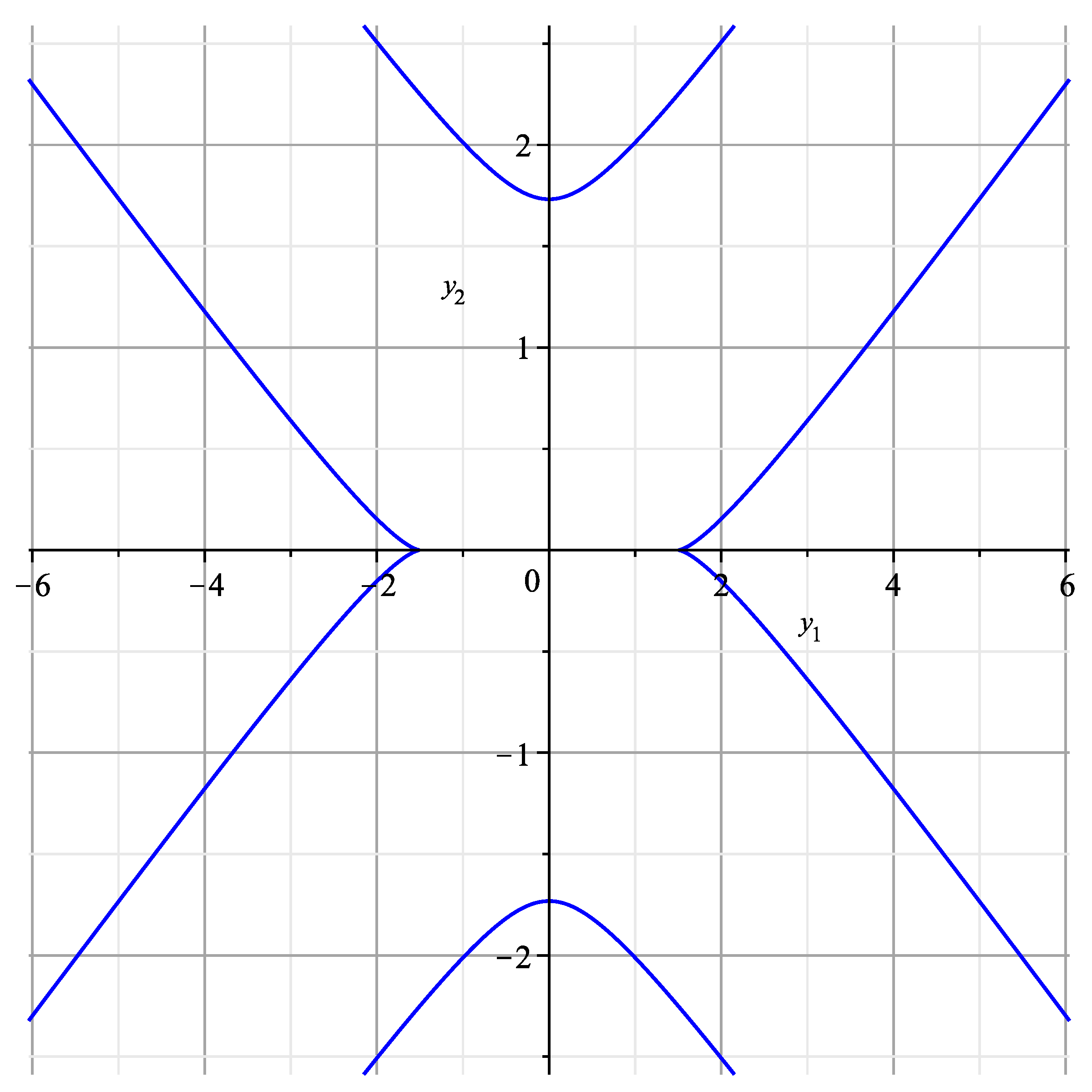
This curve is located in the band , it is symmetric relative to the axis and the vertical . When , on it , (i.e., on the curve and ). In this . At , , at , , and .
Presently, to describe the structure of variety near the line , we substitute (38) into the polynomial and obtain the polynomial . It splits into the sum
with ; using the coeff command, we obtain
In the polynomials , we substitute
We obtain a polynomial with coefficients depending on t through and . In this polynomial
where from (42), so ,
when , , and in general
according to (40). Presently, according to (41) and (43)
By generalized Theorem 1 on the implicit function, the equation has a solution as a power series over
where are rational functions that are expressed through the coefficients which in turn are expressed through and according to (44). This expansion is valid for all values of t, except maybe the roots of the function . They correspond to points , . Therefore, we have to remove them together with their neighborhoods. In particular,
where the denominator has two real roots . According to (45), approximate .
Let us return to the original coordinates, which for small on the variety are approximated by
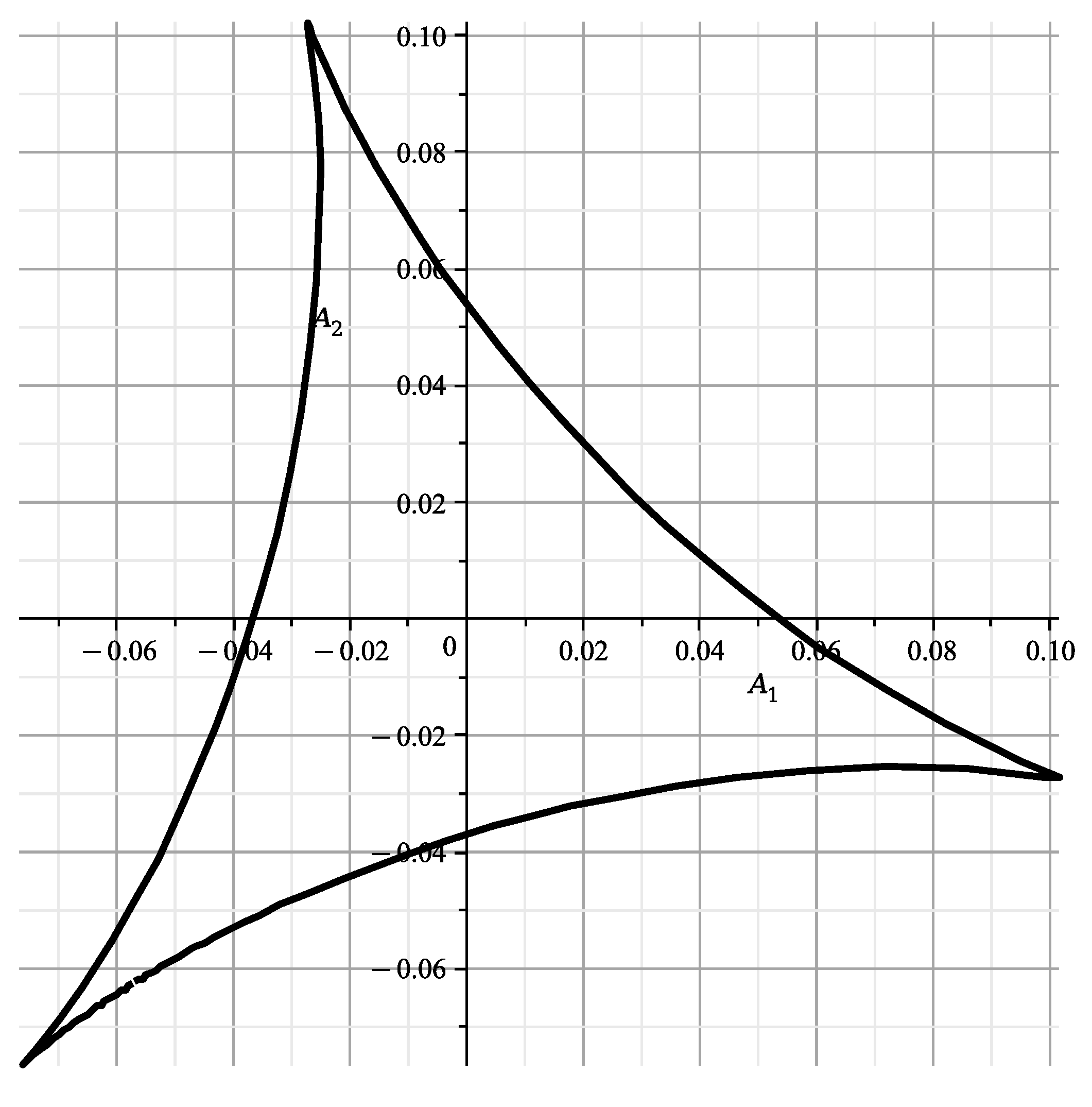
in which case
Figure 11 at (i.e., ) shows the upper and lower sections of the curve (46) and (47) for . The sections where are discarded, because they are affected by singularities of the singular points and . We observe that these curves are like parallel line segments and almost coincide. In the corresponding in Figure 12 in [25], similar branches merge.
10. The Structure of the Variety near the Singular Point
In Section 10, we moved from the coordinates to the coordinates , which are local and near the point . For the polynomial , we have already calculated the Newton polyhedron , its faces and the normals to the faces (Figure 9). There was a normal . It corresponds to a truncated polynomial
Presently, we conduct the power transformation
and obtain
Here,
The curve has genus 0, with parameterization
and its graph shown in Figure 13.
Presently, in the full polynomial , we conduct the power transformation in (49) to and extract from it all terms with in the seventh degree with the procedure mtaylor. We obtain the polynomial
Its division by will provide a polynomial , which we factorize according to the parameterization (50)
If we substitute , in , then the equation takes the form
where , ,
and in general
According to (35), in the first approximation when is small, we obtain
Author Contributions
Conceptualization, A.D.B.; methodology, A.D.B.; software, A.A.A.; validation, A.D.B.; writing—original draft preparation, A.A.A.; writing—review and editing, A.D.B.; visualization, A.A.A. All authors have read and agreed to the published version of the manuscript.
Funding
This research received no external funding.
Data Availability Statement
Not applicable.
Acknowledgments
The authors are grateful to A.B. Batkhin for his help in the software implementation of algorithms and manuscript preparation.
Conflicts of Interest
The authors declare no conflict of interest.
References
- Newton, I. A treatise of the method of fluxions and infinite series, with its application to the geometry of curve lines. In The Mathematical Works of Isaac Newton; Woolf, H., Ed.; Johnson Reprint Corp.: New York, NY, USA; London, UK, 1964; Volume 1, pp. 27–137. [Google Scholar]
- Bruno, A.D. Local Methods in Nonlinear Differential Equations; Springer: Berlin/Heidelberg, Germany; New York, NY, USA; London, UK; Paris, France; Tokyo, Japan, 1989. [Google Scholar]
- Puiseux, V. Recherches sur les fonctions algebriques. J. Math. Pures Appl. 1850, 15, 365–480. [Google Scholar]
- Liouville, J. Sur la determination des integrales dont la valeur est algebrique. J. l’Ecole Polytech. 2009, 1833, 124–193. [Google Scholar]
- Briot, C.; Bouquet, T. Recherches sur les proprietes des equations differentielles. J. l’Ecole Polytech. 1856, 21, 133–199. [Google Scholar]
- Chebotarev, N. The “Newton polygon” and its role in current developments in mathematics. In Isaak Newton; Izd. Akad. Nauk SSSR: Moscow/Leningrad, Russia, 1943; pp. 99–126. (In Russian) [Google Scholar]
- Abhyankar, S.S.; Tzuong-tsieng, M. Newton-Puiseux expansion and generalized Tschirnhausen transformation. I, II. J. Reine Angew. Math. 1973, 260, 47–83. [Google Scholar] [CrossRef]
- Bruno, A.D. The asymptotic behavior of solutions of nonlinear systems of differential equations. Soviet Math. Dokl. 1962, 3, 464–467. [Google Scholar]
- Sathaye, A. Generalized Newton-Puiseux Eexpansion and Abhyankar-Moh semigroup theorem. Invent. Math. 1983, 74, 149–157. [Google Scholar] [CrossRef]
- McDonald, J. Fiber polytopes and fractional power series. J. Pure Appl. Algebra 1995, 104, 213–233. [Google Scholar] [CrossRef]
- Weierstrass, K. Theorie der Abelshen Transcendenten. In Math. Werke; Mayer und Muller: Berlin, Germany, 1902; Volume 4, pp. 11–45. [Google Scholar]
- Hironaka, H. Resolution of singularities of an algebraic variety over a field of characteristic zero: I, II. Ann. Math. 1964, 79, 109–203. [Google Scholar] [CrossRef]
- Bruno, A.D. Power Geometry in Algebraic and Differential Equations; Elsevier Science: Amsterdam, The Netherlands, 2000. [Google Scholar]
- Bruno, A.D.; Azimov, A.A. Computing unimodular matrices of power transformations. Program. Comput. Softw. 2023, 49, 32–41. [Google Scholar] [CrossRef]
- Bruno, A.D. Algorithms for solving an algebraic equation. Program. Comput. Softw. 2018, 44, 533–545. [Google Scholar] [CrossRef]
- Kollár, J. Lectures on Resolution of Singularities; Annals of Mathematic Studies; Princeton University Press: Princeton, NJ, USA; Oxford, UK, 2007. [Google Scholar]
- Besse, A.L. Einstein Manifolds; Springer: Berlin, Germany, 1987. [Google Scholar]
- Abiev, N.A.; Arvanitoyeorgos, A.; Nikonorov, Y.G.; Siasos, P. The dynamics of the Ricci flow on generalized Wallach spaces. Differ. Geom. Appl. 2014, 35, 26–43. [Google Scholar] [CrossRef]
- Abiev, N.A.; Arvanitoyeorgos, A.; Nikonorov, Y.G.; Siasos, P. The Ricci flow on some generalized Wallach spaces. In Geometry and Its Applications; Rovenski, V., Walczak, P., Eds.; Springer: Berlin/Heidelberg, Germany, 2014; Volume 72, pp. 3–37. [Google Scholar]
- Abiev, N.A.; Arvanitoyeorgos, A.; Nikonorov, Y.G.; Siasos, P. The normalized Ricci flow on generalized Wallach spaces. In Mathematical Forum; Studies in Mathematical Analysis; Yuzhnii Matematicheskii Institut, Vladikavkazskii Nauchnii Tsentr Ross. Akad. Nauk: Vladikavkaz, Russia, 2014; Volume 8, pp. 25–42. (In Russian) [Google Scholar]
- Chen, Z.; Nikonorov, Y.G. Invariant Einstein metrics on generalized Wallach spaces. arXiv 2015, arXiv:1511.02567. [Google Scholar] [CrossRef]
- Abiev, N.A. On topological structure of some sets related to the normalized Ricci flow on generalized Wallach spaces. Vladikavkaz Math. J. 2015, 17, 5–13. [Google Scholar]
- Abiev, N.A.; Nikonorov, Y.G. The evolution of positively curved invariant Riemannian metrics on the Wallach spaces under the Ricci flow. Ann. Glob. Anal. Geom. 2016, 50, 65–84. [Google Scholar] [CrossRef]
- Nikonorov, Y.G. Classification of generalized Wallach spaces. Geom. Dedic. 2016, 111, 193–212, Correction in: Geom. Dedic. 2021, 214, 849–851. [Google Scholar] [CrossRef]
- Bruno, A.D.; Batkhin, A.B. Investigation of a real algebraic surface. Program. Comput. Softw. 2015, 41, 74–82. [Google Scholar] [CrossRef]
- Batkhin, A.B. A real variety with boundary and its global parameterization. Program. Comput. Softw. 2017, 43, 75–83. [Google Scholar] [CrossRef]
- Batkhin, A.B. Parameterization of the Discriminant Set of a Polynomial. Program. Comput. Softw. 2016, 42, 65–76. [Google Scholar] [CrossRef]
- Sendra, J.R.; Sevilla, D. First steps towards radical parametrization of algebraic surfaces. Comput. Aided Geom. Des. 2013, 30, 374–388. [Google Scholar] [CrossRef]
- Thompson, I. Understanding Maple; Cambridge University Press: Cambridge, UK, 2016. [Google Scholar]
Figure 1.
Graph of the polyhedron .

Figure 2.
Plot of the curve .

Figure 3.
Plot of the curve (21) for .
Figure 3.
Plot of the curve (21) for .

Figure 4.
Plot of the curve (21) for .
Figure 4.
Plot of the curve (21) for .

Figure 5.
The graph of the polyhedron .

Figure 6.
Plot of the curve .

Figure 7.
Plot of the curve (34) for .
Figure 7.
Plot of the curve (34) for .

Figure 8.
Plot of the curve (34) for .
Figure 8.
Plot of the curve (34) for .

Figure 9.
The graph of the polyhedron .

Figure 10.
Plot of the curve .


Figure 13.
Plot of the curve .

Figure 14.
Plot of the curve (54) for .
Figure 14.
Plot of the curve (54) for .

Disclaimer/Publisher’s Note: The statements, opinions and data contained in all publications are solely those of the individual author(s) and contributor(s) and not of MDPI and/or the editor(s). MDPI and/or the editor(s) disclaim responsibility for any injury to people or property resulting from any ideas, methods, instructions or products referred to in the content. |
© 2023 by the authors. Licensee MDPI, Basel, Switzerland. This article is an open access article distributed under the terms and conditions of the Creative Commons Attribution (CC BY) license (https://creativecommons.org/licenses/by/4.0/).
Share and Cite
MDPI and ACS Style
Bruno, A.D.; Azimov, A.A. Parametric Expansions of an Algebraic Variety near Its Singularities. Axioms 2023, 12, 469. https://doi.org/10.3390/axioms12050469
AMA Style
Bruno AD, Azimov AA. Parametric Expansions of an Algebraic Variety near Its Singularities. Axioms. 2023; 12(5):469. https://doi.org/10.3390/axioms12050469
Chicago/Turabian StyleBruno, Alexander D., and Alijon A. Azimov. 2023. "Parametric Expansions of an Algebraic Variety near Its Singularities" Axioms 12, no. 5: 469. https://doi.org/10.3390/axioms12050469
Note that from the first issue of 2016, this journal uses article numbers instead of page numbers. See further details here.