
Extremal Graphs for Sombor Index with Given Parameters
College of Mathematics and System Sciences, Xinjiang University, Urumqi 830046, China
*
Author to whom correspondence should be addressed.
Axioms 2023, 12(2), 203; https://doi.org/10.3390/axioms12020203
Submission received: 10 January 2023
/
Revised: 3 February 2023
/
Accepted: 9 February 2023
/
Published: 15 February 2023
(This article belongs to the Special Issue Graph Theory and Discrete Applied Mathematics)
Abstract
:In this paper, we present the upper and lower bounds on Sombor index among all connected graphs (respectively, connected bipartite graphs). We give some sharp lower and upper bounds on among connected graphs in terms of some parameters, including chromatic, girth and matching number. Meanwhile, we characterize the extremal graphs attaining those bounds. In addition, we give upper bounds on among connected bipartite graphs with given matching number and/or connectivity and determine the corresponding extremal connected bipartite graphs.
MSC:
05C50; 05C12; 15A181. Introduction
In this paper, we only consider finite, undirected and simple connected (respectively, connected bipartite) graphs. Let G be a graph with vertex set and edge set . Let S (respectively, F) be a vertex (respectively, an edge) subset of G. Then denotes the graph obtained from G by deleting S and the edges incident with them, and denotes the graph obtained from G by deleting F. If and , the subgraphs and will be written as and for short, respectively. For any two nonadjacent vertices x and y of a graph G, we let be the graph obtained from G by adding an edge . For a positive integer n, we will use the notation .
Recently, Gutman [1] devised two new topological indices. For a graph G, its Sombor index and reduced Sombor index are defined, respectively, as follows:
Gutman et al. [1] studied the problem of finding graphs attaining the maximum (respectively, minimum) Sombor index from the class of all trees (respectively, graphs and connected graphs) with given order n. Réti et al. [2] characterized the extremal graphs having the maximum Sombor index in the classes of all connected unicyclic, bicyclic, tricyclic, tetracyclic, and pentacyclic graphs with order n.
Liu et al. [3] obtained some bounds for the reduced Sombor index of graphs with given several parameters and some special graphs. F. Wang and B. Wu [4] proved a conjecture on the reduced Sombor index proposed by Liu et al. in [3]. They gave an upper bound for the reduced Sombor index of a bipartite graph and determined the extremal graph among all k-chromatic graphs with maximum reduced Sombor index. F. Wang and B. Wu [5] characterized the extremal molecular tree on the reduced Sombor index and exponential reduced Sombor index.
Some authors made a more extensive study to determine the extremal values of the Sombor index of graphs with given some parameters. Sun et al. [6] characterized extremal graphs having extremal values of the Sombor index in terms of the domination number. In [7], Zhou et al. characterized the extremal trees and unicyclic graphs with the extremal Sombor index in terms of the matching number. They also considered the extremal Sombor index in the same graph family with given maximum degree in [8]. Das et al. [9] gave some bounds on the Sombor index of trees in terms of order, independence number, and number of pendent vertices, and characterized the extremal cases. Liu et al. [10] collected the existing bounds and extremal results related to the Sombor index and its variants. Aashtab et al. [11] found an interesting property of the Sombor index. Let G be a connected graph of order n and size m, if for each with order n and size m, , then G is an almost regular graph. Using this property, Liu et al. [12] determined the minimum Sombor index of tricyclic and tetracyclic graphs.
If there exists a vertex such that is a tree (respectively, unicycle), then the graph G is said to be a quasi-tree (respectively, quasi-unicyclic). Das et al. [9] determined the extremal graphs in the set of quasi-trees. Ning et al. [13] gave an upper bound of the Sombor index of the set of quasi-unicyclic graphs with order n, and characterized the corresponding extremal graph. Horoldagva et al. [14] gave some lower or upper bounds on the Sombor index of connected graphs in terms of some parameters, such as the maximum degree. Das et al. [15] gave an upper bound of the Sombor index of connected graphs with a given independence number. Some authors obtained a series of results related to Nordhaus–Gaddum relations for the Sombor index in [14,15,16].
The extremal values of the Sombor index of chemical graphs are also studied by several authors. A chemical graph is a graph with the degree of each vertex of this graph at most 4. Deng et al. [17] gave an upper bound of the Sombor index in chemical trees with n vertices. Cruz et al. [18] characterized the extremal connected chemical graphs of order n, and determined the extremal graphs in catacondensed hexagonal systems. Liu et al. [19] gave lower and upper bounds of the Sombor index in chemical trees with n vertices and k pendent vertices, and characterized the corresponding extremal chemical trees. Liu et al. [20] determined the first fourteen minimum chemical trees, the first four minimum chemical unicyclic graphs, the first three minimum chemical bicyclic graphs, and the first seven minimum chemical tricyclic graphs.
Some authors considered the relationships between the Sombor index and other indices. Filipovski et al. [21] considered the relations between the Sombor index and some degree-based topological indices. Rata et al. [22] considered the relationship between the Sombor index and the Second Zagreb index.
Recently, Réti et al. [2] introduced a new notion, called k-Sombor index of a graph as follows. For a positive real number k, the k-Sombor index of graph G, denoted by , is defined as
F. Wang, B. Wu [23] presented the extremal values of the k-Sombor index of trees with some given parameters, such as matching number, the number of pendent vertices, and diameter. Some related results about the Sombor index can be found in [24,25,26].
In this paper, we present the upper and lower bounds on among all connected graphs (respectively, bipartite graphs). In Section 3, we consider some extremal problems on with given parameters, such as chromatic number, girth and matching number among connected graphs. In Section 4, we give some sharp upper bounds on the in bipartite graphs with given matching number and connectivity. In addition, we characterize the extremal graphs attaining these bounds. In Section 5, we conclude our paper.
2. Preliminaries
For two sets A and B of vertices of G, we write for the set of edges with and . An induced subgraph is the subgraph of G whose vertex set is A and whose edge set consists of all edges of G which have both ends in A. If F is a set of edges, the edge-induced subgraph is the subgraph of G whose edge set is F and whose vertex set consists of all ends of edges of F. If , we denote by the graph, which consists of two components and . The join of and , denoted by , is the graph with vertex set and edge set . A matching of G is a subset of mutually independent edges of G. For a graph G, the matching number is the maximum cardinality among the independent sets of edges in G.
A graph G is called k-connected if is connected for every subset with . The greatest integer k such that G is k-connected is the connectivity of G.
Throughout this paper, we use and to denote the path graph, star graph, cycle graph, complete graph, and independence set on n vertices, respectively.
In what follows, we give some lemmas which will be used frequently in the proofs of the main results.
Proposition 1.
Let G be a connected graph with at least three vertices.
(a) If then where ;
(b) If G has an edge e not being a cut edge, then .
Lemma 1
([1]). Let be the path of order n. Then for any connected graph G of order n,
Equality holds if and only if or . Moreover, , whereas for
Lemma 2
([1]). Let be the star of order n. Then for any tree T of order n.
Equality holds if and only if or . Moreover, .
Lemma 3
([27]). Every k-chromatic graph has at least k vertices of degree at least .
Lemma 4.
(The Tutte-Berge Formula) For any graph G:
Lemma 5.
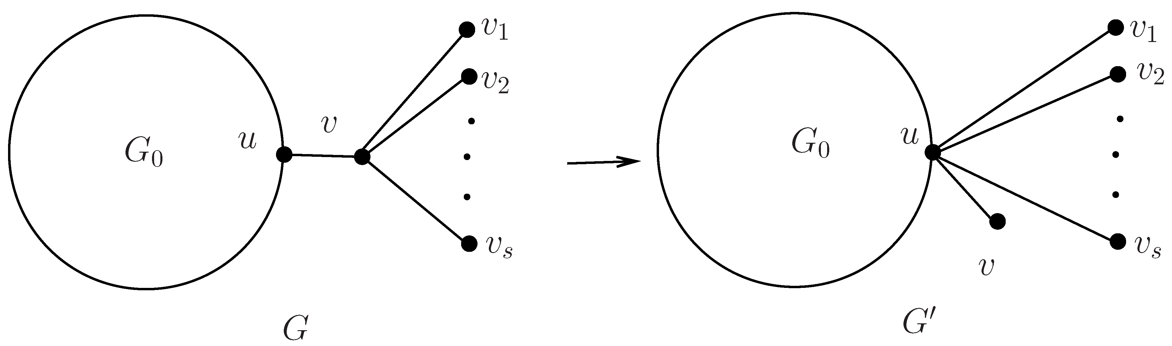
Suppose that is a nontrivial connected graph. Let G be a graph obtained from by connecting a central vertex to a vertex . Let be a graph obtained from G by deleting all edges of and connecting each vertex of , apart from v, to u, see Figure 1. Then
Proof.
Consider the difference between and .
□
3. Connected Graphs with Given Parameters
3.1. Extremal Graphs with Regard to in Terms of Order n and Chromatic Number c
Let be the set of connected graphs on n vertices with chromatic number c. A c-partite graph is complete if any two vertices in different parts are adjacent. A simple complete c-partite graph on n vertices whose parts are of equal or almost equal sizes (that is, or ) is called a and denoted by . We consider the extremal value of of graphs G from , and determine the corresponding extremal graphs.
In [28], Das et al. gave an upper bound on in terms of order n and chromatic number c, and characterized the extremal graphs in the following theorem. The extremal graph is exactly the Turán graph .
Theorem 1
Moreover, .
In what follows, we give a lower bound on in terms of order n and chromatic number c, and characterize the extremal graph in the following theorem. Denote by a connected graph obtained from by attaching a path to a vertex .
Theorem 2.
Let with . Then
the equality holds if and only if .
Proof.
Suppose that ) is a graph having minimum value of . Let . Since G has chromatic number c, by Lemma 3, there is a vertex subset with cardinality at least c. Moreover, the degree of each vertex is at least . According to the definition of and Proposition 1, it is easy to see that the value of decreases when deleting edges in G. It implies that the value of G reaches its minimum when the graph G contains as few edges as possible. Based on these facts, we conclude that is a complete subgraph . Note that the graph G contains as few edges as possible, and each vertex v belongs to S with . We have that contains as few edges as possible. Thus, must be a union of some trees. Thus, , where is a tree containing as its root in for and . Denote by the graph obtained from by attaching a vertex of tree to a vertex of for .
Without loss of generality, suppose that , . Let for and .
For each subscript , by repeating the use of Lemma 5, we obtain a new graph obtained from by attaching a path to for . It is not difficult to see that .
Replacing the clique in with a copy of , namely , we obtain a new - tree with . In fact, is isomorphic to a tree T. By Lemma 2, we can obtain a new tree from T such that and . In what follows, we consider two cases of whether is an end vertex of or not.
Case 1. .
In this case, we replace (respectively, T) by to obtain a graph (respectively, ). According to the result obtained above, we obtain immediately. It is easy to see that . The result holds.
Case 2. .
In this case, we replace by to obtain a new graph . Let p and q be two positive integers. The graph can be viewed as a graph obtained from by attaching two paths and to two distinct vertices and of for .
Let and . Suppose that . Consider the Sombor index of . Let and consider the Sombor index of .
The expression of is independent of p and q. This implies that . In what follows, compare the difference between and :
Thus, . Since , we know that is exactly the extremal graph with a minimum value of in this case.
Combining the two cases above, we complete the proof of Theorem 2. □
3.2. Extremal Graphs with Regard to in Terms of Order n and Girth g
Let be the set of all connected graphs with given order n and girth g. In this subsection, we characterize the extremal graph having a minimum value of the Sombor index in .
Let be a cycle of length g. Denote by the graph obtained by connecting a pendent vertex of a path with one vertex .
Theorem 3.
Let . Then
and the equality holds if and only if . Moreover, .
Proof.
Suppose that is a graph with a minimum value of . Let be the shortest cycle of G. We first claim that the cycle is the only cycle of G. In fact, suppose, to the contrary, that there exists another cycle different from , where . By Proposition 1, we know that deleting edges will decrease the value of . Delete an edge of , and then we obtain a new graph satisfying . It is easy to see that , a contradiction.
By Proposition 1 and the choice of G, it is easy to see that contains as few edges as possible. Based on the analysis above, we know that must be a forest. Let . Denote by the tree containing in , where . There exist some trees being single vertices. Without of loss generality, suppose that are trees of order at least 2, where .
Replace the cycle in G by a copy of and denote it by . We obtain a new graph with . In fact, is isomorphic to a tree T. By Lemma 2, we can obtain a new tree from T such that and . In what follows, we consider two cases whether is an end vertex of or not.
Case 1. .
In this case, we replace (respectively, T) by to obtain a graph (respectively, ). According to the result obtained above, , we obtain immediately. It is easy to see that . The result follows.
Case 2. .
Let and be two integers. We replace by to obtain a new graph . We see that can be viewed as two paths and connected to two distinct vertices and of cycle , respectively. Note that . Suppose that . Denote by a new graph obtained by deleting the edge between and the path , and attaching to anther end vertex of . We know that can be viewed as a graph obtained by connecting a path to any vertex of . Note that . Next, compare the difference between and :
Thus, we have . In this case, has the minimum value of .
Combing the two cases, we conclude that has a minimum value of in . This completes the proof of this theorem. □
Let . By Proposition 1, adding edges increases the value of the Sombor index. It is easy to see that G contains as many edges as possible. Thus, . The equality holds if and only if . Moreover, . If , it is difficult to determine the extremal graphs having a maximum value of the Sombor index in .
3.3. Extremal Graphs with Regard to in Terms of Matching Number
Let be the set of connected graphs of order n and matching number . In what follows, we will determine the extremal graph G in with maximum , and calculate the corresponding value of .
Firstly, consider some special cases. If and , then . If and , then . Moreover, and . So, in what follows, we always assume that and .
If and , then . The left equality holds if and only if and the right equality holds if and only if . Moreover, and
Theorem 4.
Let . If and , then
the equality holds if and only if .
Moreover,
Proof.
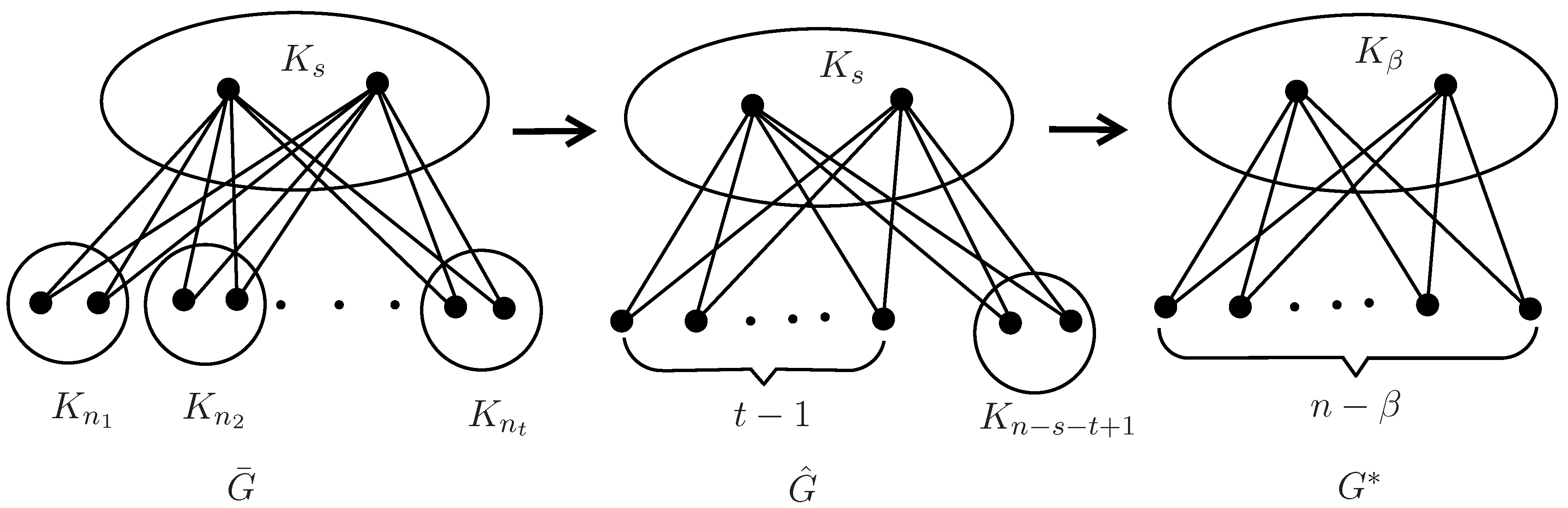
We characterize the structure of extremal graph with maximum . Suppose t and s are two positive integers. Let , be all odd positive integers.
We first show that . Let . Suppose that there exists a graph having the maximum . According to Lemma 4, we conclude that there exists a set with , such that contains t odd components and . Note that and then . Since , we have . Thus, .
Suppose that . Let . It is easy to see that is a union of even components of . If , we add edges to until there are no edges to add to this induced subgraph. That is, the induced subgraph is a clique . Denote by the resulting graph obtained from by adding as many edges as possible in . By Lemma 4, we have . According to the fact that adding edges in any graph does not reduce the matching number, we have Then, we have Thus, . Since the number of edges in are more than the number of edges in . By Proposition 1, we have . This contradicts the choice of .
If , then . According to the assumption that , we can obtain a new graph from by adding edges between each pair vertex sets S and , , and adding edges in and . According to Proposition 1, we have . This contradicts the maximality of .
Combining above two cases, we have .
According to the fact above, we know that is the extremal structure in with maximum value of .
Next, let us conduct further analysis to determine the specific value of each for and optimize the graph such that the value of becomes as large as possible. Consider the value of , and we have
Define a function with t variables as the following.
, where is constant. Suppose , and for . Consider the following formula:
Define two functions as following
.
Taking the first derivative, we have
.
Since , we have and . It is easy to see that .
From the above, we see that the function increases when the pair changes by the following chain .
For any pair , , if , we repeat the above process until the graph (i.e., ) becomes a new graph (i.e., ). The graphs and are given in Figure 2. By Proposition 1, we obtain .
Next, continue to increase the value of . Notice that . We calculate this value by the following:
Let , with . Taking the first derivative, we have .
For , we check that . That is, the function is increasing when . Then, we conclude that reaches its maximum value at with . Note that (see Figure 2) for , and then .
That is, .
This completes the proof. □
4. Bipartite Graphs with Given Parameters
4.1. Extremal Bipartite Graphs with Regard to in Terms of Matching Number
Let be the class of all bipartite graphs of order n and matching number . In this subsection, we give some upper bounds on of all connected graph . Meanwhile, we determine the corresponding extremal graphs.
Theorem 5.
Let . Then
the equality holds if and only if . Moreover,
Proof.
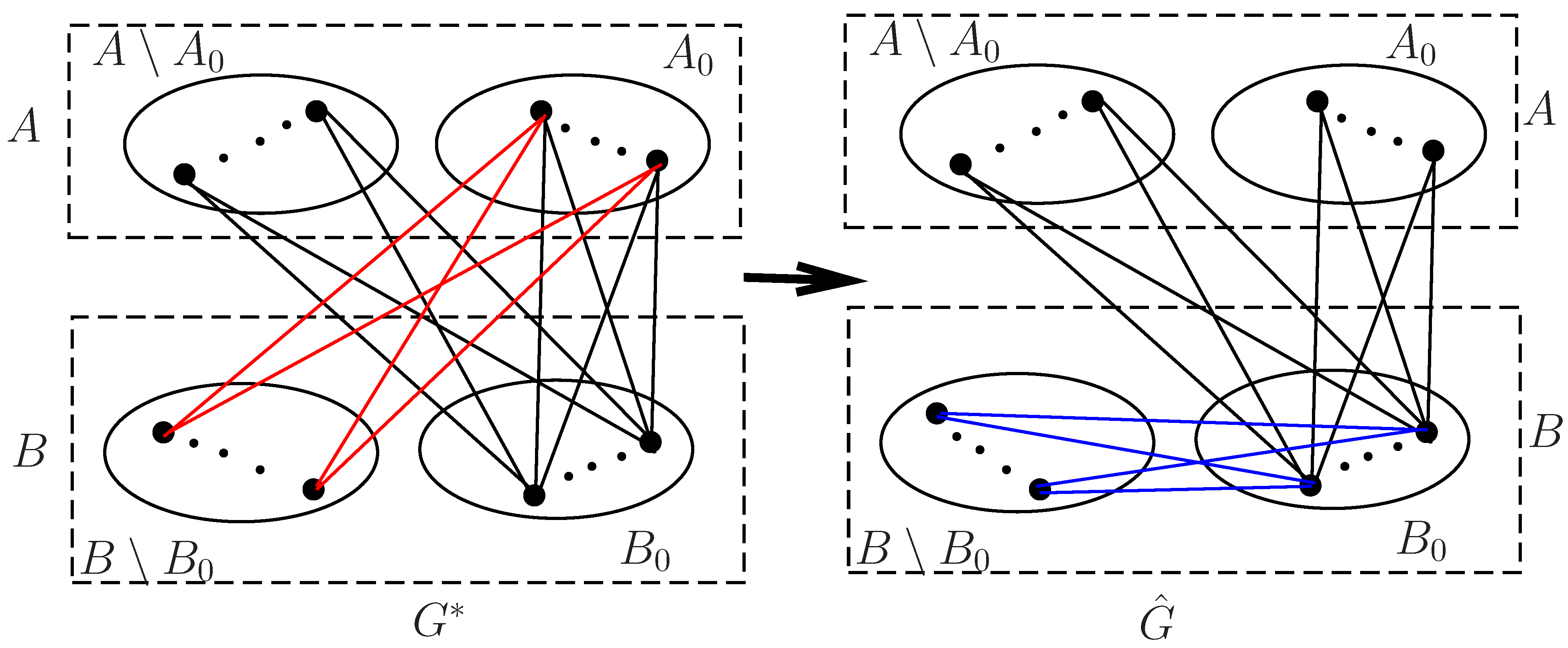
Suppose that is an extremal graph with maximum . Let be the bipartition of the vertex set of G, and . Let M be a maximal matching of G, and . Suppose . Let , and . It is easy to see that . Since , we consider two cases depending on the value of . If , then and . We claim that . Suppose, to the contrary, that . Construct a new graph obtained from G by adding edges between two sets A and B. According to Proposition 1, adding edges will increase the value of the Sombor index, and then we have . This contradicts the choice of G. Thus, .
If and , then . In what follows, we assume that . We show that . Otherwise, if there exists an edge , then we find a new matching . Thus, . This is a contradiction. Construct a new graph from G by adding as many edges as possible between the two sets and (respectively, and , and ). We have . Note that and . It is easy to see that , and . Choose as a proper subset of maximum matching of . That is, . Since and , we can find maximal matching with order in . Hence, and . Next, construct a new graph from by deleting red edges and adding blue edges such that , and . The graphs and are given in Figure 3. It is easy to check that with .
In what follows, we claim that . Compare the difference between and :
Thus, . This implies that .
We complete the proof of the Theorem 5. □
Figure 3.
The graphs used in the proof of the Theorem 5.

4.2. Extremal Bipartite Graphs with Regard to in Terms of Connectivity k
Let be the class of all bipartite graphs of order n and connectivity k. In what follows, we determine the extremal graphs in with the maximum Sombor index. Denote by the complete bipartite graph with two partitions A and B. Let . In [29], Li et al. gave two definitions of two operations and . Denote by the graph obtained by connecting each vertex of to each vertex of one partition with order (respectively, ) of (respectively, ). Denote by the graph obtained by connecting each vertex of to each vertex of one partition with order (respectively, ) of (respectively, ).
Theorem 6.
Let with .
(I) If or , then .
Moreover,
(II) If , then for some p and q.
Moreover, .
Proof.
Suppose that G is a graph in with maximum . Let S be a minimal vertex cut set with , and be the connected components of , where . If there exists such that , then must be a complete bipartite subgraph. Otherwise, we can obtain a new graph obtained from G by adding edges in . By Proposition 1, adding edges increases the value of the Sombor index, we have . This contradicts the choice of G. If there exists such that , then must be a complete bipartite subgraph . Otherwise, we can find a smaller vertex cut set than S such that the connectivity of G is less than k. This is a contradiction. Moreover, . If there exists an edge , then we can find a triangle in G, a contradiction.
Case 1 or .
In this case, each component of must be a single vertex . Otherwise, suppose that there exists a component with for . Obviously, is a complete bipartite subgraph. Denote by A the partition of such that A and S are in different partition of G. It is easy to see that A is a vertex cut set with . This is a contradiction. Thus, . Then, .
Case 2 .
We claim that contains exactly two components and . Otherwise, suppose that . Since each component with order at least 2 is a complete bipartite subgraph, we can obtain a new graph obtain from G by adding edges in such that becomes a complete bipartite subgraph. By Proposition 1, we obtain a contradiction that .
Without loss of generality, let , and . Let be two partitions of with , and . Let . It is easy to see that . Otherwise, X is a vertex cut set with . This is a contradiction.
Calculate the Sombor index of .
□
5. Concluding Remarks
In this paper, we give some further results on . We determine the upper and lower bounds on among general connected graphs in terms of several graph parameters, i.e., chromatic number, and characterize the extremal graphs. In addition, we consider the extremal value of the Sombor index in bipartite graphs in terms of connectivity and matching number, and determine the corresponding extremal bipartite graphs.
Naturally, it is interesting to consider the extremal connected bipartite graphs in terms of other parameters. We state a few challenging open problems on Sombor index for connected graphs and connected bipartite graphs.
Problem 1.
Determine an upper bound on Sombor index for connected graphs in terms of girth.
Problem 2.
How can we determine lower and upper bounds on Sombor index for connected bipartite graphs in terms of diameter.
Problem 3.
Determine lower and upper bounds on Sombor index for connected bipartite graphs in terms of radius.
Problem 4.
Determine lower and upper bounds on the Sombor index for connected bipartite graphs in terms of domination.
Our research on the Sombor index among connected graphs and connected bipartite graphs with some given parameters is just the beginning. We will continue to conduct research along this line in the future.
Author Contributions
Writing and editing, W.Z.; supervision and review, J.M.; conceptualization, N.W.; funding acquisition, J.M. All authors have read and agreed to the published version of the manuscript.
Funding
This research is supported by the Natural Science Foundation of Xinjiang (No. 2020D04046).
Data Availability Statement
No data, models, or code were generated or used during the study.
Conflicts of Interest
The authors declare no conflict of interest.
References
- Gutman, I. Geometric approach to degree-based topological indices: Sombor indices. MATCH Commun. Math. Comput. Chem. 2021, 86, 11–16. [Google Scholar]
- Réti, T.; Doslic, T.; Ali, A. On the Sombor index of graphs. Contrib. Math. 2021, 3, 11–18. [Google Scholar]
- Liu, H.C.; You, L.H.; Tang, Z.K.; Liu, J.B. On the reduced Sombor index and its applications. MATCH Commun. Math. Comput. Chem. 2021, 86, 729–753. [Google Scholar]
- Wang, F.X.; Wu, B. The Proof of a Conjecture on the Reduced Sombor Index. MATCH Commun. Math. Comput. Chem. 2022, 88, 583–591. [Google Scholar] [CrossRef]
- Wang, F.X.; Wu, B. The reduced Sombor index and the exponential reduced Sombor index of a molecular tree. J. Math. Anal. Appl. 2022, 515, 126442. [Google Scholar] [CrossRef]
- Sun, X.; Du, J. On Sombor index of trees with fixed domination number. Appl. Math. Comput. 2022, 421, 126946. [Google Scholar] [CrossRef]
- Zhou, T.; Lin, Z.; Miao, L. The Sombor index of trees and unicyclic graphs with given matching number. arXiv 2021, arXiv:2103.04645. [Google Scholar] [CrossRef]
- Zhou, T.; Lin, Z.; Miao, L. The Sombor index of trees and unicyclic graphs with given maximum degree. arXiv 2021, arXiv:2103.07947. [Google Scholar]
- Das, K.C.; Gutman, I. On Sombor index of trees. Appl. Math. Comput. 2022, 412, 12675. [Google Scholar] [CrossRef]
- Liu, H.; Gutman, I.; You, L.; Huang, Y. Sombor index:review of extremal results and bounds. J. Math. Chem. 2022, 60, 771–798. [Google Scholar] [CrossRef]
- Aashtab, A.; Akbari, S.; Madadinia, S.; Noei, M.; Salehi, F. On the graphs with minimum Sombor index. MATCH Commun. Math. Comput. Chem. 2022, 88, 553–559. [Google Scholar] [CrossRef]
- Liu, H.; You, L.; Huang, Y. Extremal Sombor indices of tetracyclic (chemical) graphs. MATCH Commun. Math. Comput. Chem. 2022, 88, 573–581. [Google Scholar] [CrossRef]
- Ning, W.; Song, Y.; Wang, K. More on Sombor index of graphs. Mathematics 2022, 10, 301. [Google Scholar] [CrossRef]
- Horoldagva, B.; Xu, C. On Sombor index of graphs. MATCH Commun. Math. Comput. Chem. 2021, 86, 703–713. [Google Scholar]
- Das, K.C.; Cevik, A.S.; Cangul, I.N.; Shang, Y. On Sombor index. Symmetry 2021, 13, 140. [Google Scholar] [CrossRef]
- Ghanbari, N.; Alikhani, S. Sombor index of certain graphs. Iran. J. Math. Chem. 2021, 12, 27–37. [Google Scholar]
- Deng, H.; Tang, Z.; Wu, R. Molecular trees with extremal values of Sombor indices. Int. J. Quantum Chem. 2021, 121, e26622. [Google Scholar] [CrossRef]
- Cruz, R.; Gutman, I.; Rada, J. Sombor index of chemical graphs. Appl. Math. Comput. 2021, 399, 126018. [Google Scholar] [CrossRef]
- Liu, H.; Chen, H.; Xiao, Q.; Fang, X.; Tang, Z. More on Sombor indices of chemical graphs and their applications to the boiling point of benzenoid hydrocarbons. Int. J. Quantum Chem. 2021, 121, 26689. [Google Scholar] [CrossRef]
- Liu, H.; You, L.; Huang, Y. Ordering chemical graphs by Sombor indices and its applications. MATCH Commun. Math. Comput. Chem. 2022, 87, 5–22. [Google Scholar] [CrossRef]
- Filipovski, S. Relations between Sombor index and some degree-based topological indices. Iran. J. Math. Chem. 2021, 12, 19–26. [Google Scholar]
- Rada, J.; Rodriguez, J.M.; Sigarreta, J.M. General properties on Sombor indices. Discrete Appl. Math. 2021, 299, 87–97. [Google Scholar] [CrossRef]
- Wang, F.X.; Wu, B. The k-Sombor index of trees. Asia-Pac. J. Oper. Res. 2023. [Google Scholar] [CrossRef]
- Chen, H.; Li, W.; Wang, J. Extremal Values on the Sombor Index of Trees. MATCH Commun. Math. Comput. Chem. 2022, 87, 23–49. [Google Scholar] [CrossRef]
- Milovanović, I.; Milovanović, E.; Matejić, M. On some mathematical properties of Sombor indices. Bull. Int. Math. Virtual Inst. 2021, 11, 341–353. [Google Scholar]
- Xu, K.; Das, K.C. Some extremal graphs with respect to inverse degree. Discrete Appl. Math. 2016, 203, 171–183. [Google Scholar] [CrossRef]
- Bondy, J.A.; Murty, U.S.R. Graph Theory with Applications; Macmillan Press: New York, NY, USA, 1976. [Google Scholar]
- Das, K.C.; Shang, Y. Some extremal graphs with respect to Sombor index. Mathematics 2021, 9, 1202. [Google Scholar] [CrossRef]
- Li, S.; Song, Y. On the sum of all distances in bipartite graphs. Discrete Appl. Math. 2014, 169, 176–185. [Google Scholar] [CrossRef]
Figure 1.
The graphs used in the proof of the Lemma 5.

Figure 2.
The graphs used in the proof of the Theorem 4.

Disclaimer/Publisher’s Note: The statements, opinions and data contained in all publications are solely those of the individual author(s) and contributor(s) and not of MDPI and/or the editor(s). MDPI and/or the editor(s) disclaim responsibility for any injury to people or property resulting from any ideas, methods, instructions or products referred to in the content. |
© 2023 by the authors. Licensee MDPI, Basel, Switzerland. This article is an open access article distributed under the terms and conditions of the Creative Commons Attribution (CC BY) license (https://creativecommons.org/licenses/by/4.0/).
Share and Cite
MDPI and ACS Style
Zhang, W.; Meng, J.; Wang, N. Extremal Graphs for Sombor Index with Given Parameters. Axioms 2023, 12, 203. https://doi.org/10.3390/axioms12020203
AMA Style
Zhang W, Meng J, Wang N. Extremal Graphs for Sombor Index with Given Parameters. Axioms. 2023; 12(2):203. https://doi.org/10.3390/axioms12020203
Chicago/Turabian StyleZhang, Wanping, Jixiang Meng, and Na Wang. 2023. "Extremal Graphs for Sombor Index with Given Parameters" Axioms 12, no. 2: 203. https://doi.org/10.3390/axioms12020203
Note that from the first issue of 2016, this journal uses article numbers instead of page numbers. See further details here.