1. Introduction
Environmental scientists often use birds to understand ecosystems because birds are sensitive to environmental changes [
1]. As a result, there are many protected areas around the world dedicated to the conservation of bird species. However, identifying and classifying birds using conventional artificial vision is a difficult task. This is a particularly complicated problem for images where occlusion is present in uncontrolled environments.
Computer vision is a field of artificial intelligence that attempts to extract meaningful information by analyzing and processing image patterns. Additionally, this field, has several branches: classification, object localization, object detection, object recognition, and segmentation.
Object recognition is a task that identifies an object present in images or videos. It is one of the most important applications of machine learning and deep learning. The purpose of this field is to recognize the content of an image using machine learning techniques or deep learning architecture.
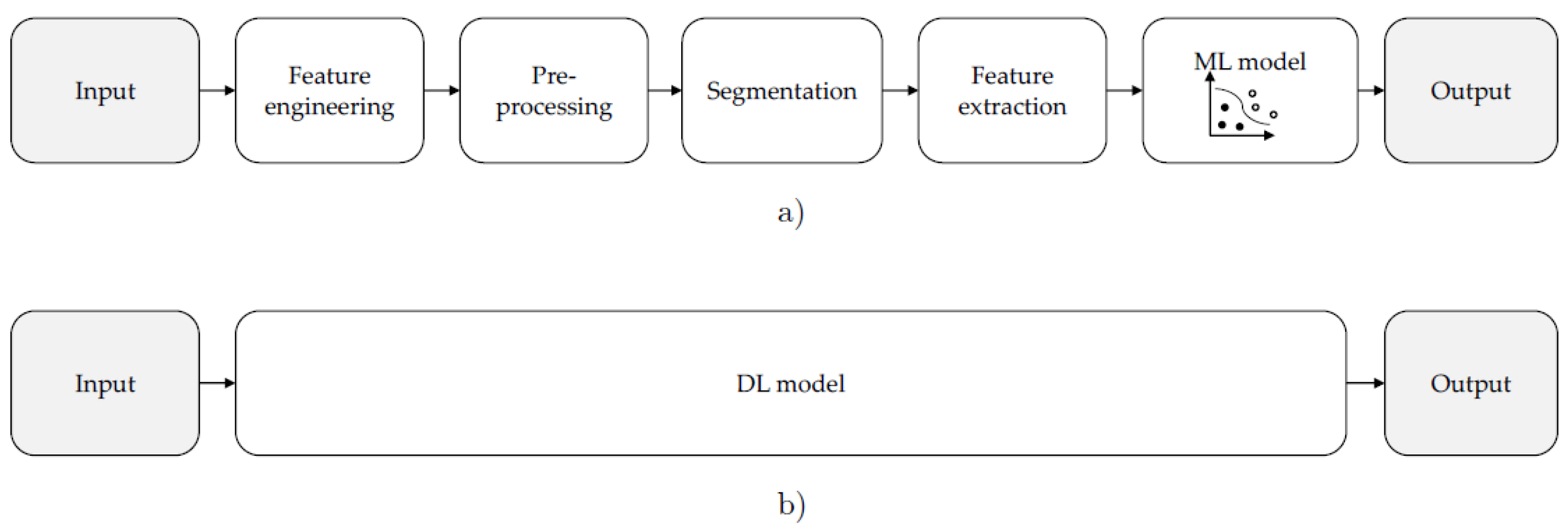
Figure 1a shows the classical computational vision methodology for object recognition in computer vision. The other alternative is to use a deep learning architecture (
Figure 1b). As we can see, the latter is less interpretable because it is equivalent to a black box where the main processes of feature extraction and selection are hidden. This paper proposes a methodology that combines elements of the two methodologies.
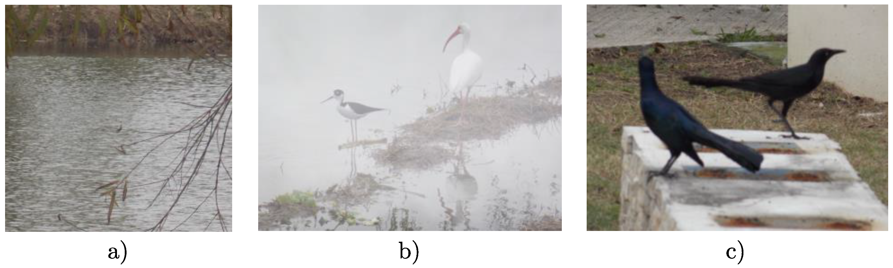
Object recognition is considered one of the critical problems because there are several challenges to deal with images, such as:
- A.
Occlusion, i.e., obscuring part of the object by equal or unequal elements of the scene,
Figure 2a.
- B.
Environmental artifacts, such as rain and fog, which can affect the quality of the image,
Figure 2b.
- C.
Uncontrolled environments are caused by the lack of a protocol for image captures, such as the object’s contrasting background, height, distance from the camera, and light correction,
Figure 2c.
Therefore, in order to recognize an object, the methodology considers tasks, such as object detection and segmentation. Segmentation is the principal problem and is our focus in this work.
The segmentation goal is to identify the pixels belonging to the target object or region of interest (ROI). However, determining the optimal number of regions per image is very time-consuming and computationally expensive. Segmentation methods based on pixel-by-pixel classification can be broadly divided into two families: semantic segmentation and instance segmentation. The first type separates all pixels that belong to the same object class. The second identifies each of the objects present in the image as an individual.
Traditionally, variable or feature selection is performed using composite variables, such as the principal component analysis technique (PCA) [
3,
4,
5] and other classification methods [
6]. Composite variables are methods that simplify the sample space of variables by normalizing linear combinations of them. However, in recent years, there have been published methods for improving feature selection by incorporating combinatorial optimization methods [
7,
8,
9,
10,
11,
12] and model selections for machine learning [
13]. For this reason, in this paper, we propose including an enhanced method for feature selection using the simulated annealing (SA) algorithm, a metaheuristic for combinatorial optimization, which is used to improve the feature set selected with the PCA technique.
We present a new methodology for object recognition called PSEV-BF (pre-segmentation and enhanced variables for bird features) that uses the pre-segmentation information before segmentation to refine the delimited area. This methodology has the phases of pre-processing, pre-segmentation, segmentation, ROI feature extraction, enhancement of relevant variables, and classification.
The rest of the paper is organized as follows.
Section 2 presents related work with a qualitative comparison of object recognition.
Section 3 presents the formulation and description of all phases of the proposed methodology.
Section 4 defines the data, performance metrics, and tools used in this work. In
Section 5, we present the proposed algorithms and their tuning method and show the application of the methodology to the dataset presented in the paper. Finally, we compare the results with the classical methodology.
Section 6 presents our conclusions.
2. Related Works
In this section, several works related to the problems of computer vision phases are discussed. For instance, in the work of [
14], a feature selection algorithm based on genetic programming (GP) is proposed. In [
14], the segmentation and classification of horses and airplane images were implemented using parsimony GP features selection (PGP-FS), nondominated sorting GP feature selection (NSGP-FS), and strength Pareto GP feature selection (SPGT-FS) algorithms. These features were subjected to the decision tree, naive Bayes, and multilayer perceptron classifiers from the Weka tool. A total of 52 features were extracted in terms of Gabor filter, color, and statistical values based on a grayscale. The accuracy, F1, precision, and recall metrics were used. The selection method shows that, on average, 15 features are selected from the original 52.
There are works related to the segmentation and classification of images of skin lesions. For instance, in [
15], the authors used the PCA technique and the Boltzmann entropy method to select a set of features. Feature selection was performed by considering the score (variance explained) of each PCA component. The features considered were color, texture, and shape, resulting in a total of 3849 features. By using PCA and Boltzmann methods, the number of features was reduced to 449. The selection of features was validated using the metrics DICE, Jaccard index, Jaccard distance, and Seg diameter. The selected features were classified using the following machine learning models: support vector machine (SVM), decision trees (DT), bagged trees (BT), subspace discriminant analysis (SDA), weighted-K nearest neighbor (W-KNN), fine-K nearest neighbor (F-KNN), subspace-K nearest neighbor (S-KNN), linear discriminant analysis (LDA), quadric discriminant analysis (QDA), cubic-support vector machine (C-SVM), and quadric-support vector machine (Q-SVM). The classifiers were validated using the metrics of sensitivity, specificity, accuracy, and F-score.
In 2018, Sharif and collaborators proposed a methodology for citrus disease detection using optimized weighted segmentation and feature selection [
16]. The processing phase consists of a top-hat filter to eliminate noise elements and a Gaussian filter to soften the image and eliminate high-intensity fluctuations. In the segmentation phase, they used a combination of segmentation techniques with weight assignment and relevance map, which allow for retaining the elements of the image with high contrast. The extracted features are related to color, texture, and geometric features, giving a total of 270 features. PCA is used to obtain a score corresponding to the explained variance of the components. Entropy and skewness are calculated for each component to select a vector of 100 features with the highest percentages. These features were obtained by training K-nearest weighted (KNN), ensemble boosted trees (EBT), DT, and LDA classifiers and then evaluating them by 10-fold. Validation of the methodology was performed using the metrics positive false rate, negative false rate, positive true rate, negative false rate, positive predictive value, false detection rate, area under the curve, and accuracy. The authors showed that their results can keep up with the current state-of-the-art methods.
Rehman et al., in 2018, applied a feature selection for image segmentation to detect glaucoma in the optic disk region using several parameters [
17]. Additionally, in pre-processing, a bilateral filter was applied to allow the removal of noise, a clipping that allows the activation of a threshold criterion to keep objects with high intensity and discard unwanted background noise, and finally, the normalization of the red (R) channel of the image to obtain information about the exciters searched. Statistical, text on the map, and fractal features were used in the segmentation phase. Then, a selection process was performed according to the method of minimal redundancy
. These features were trained using SVM, random forest (RF), AdaBoostM1, and rus boost classifiers. The model was validated using the metrics of sensitivity, specificity, similarity coefficient DICE, precision, and area overlap based on the confusion matrix, with results competing with other state-of-the-art methods.
More recently, deep-learning-based methods were used for bird detection [
18,
19,
20,
21,
22], classifying bird images [
23], and recognizing birds [
24]. For instance, [
21] used the convolutional neural network (CNN) and you only look once V3 (YOLOV3) for the detection of birds from images. In this work, the authors propose a CNN with similar architecture to the Darknet-53 network. The model was validated using the accuracy metric and comparing it with similar architectures, such as region-based convolutional neural network (R-CNN), VGG-16 + SVM, and YOLO. Additionally, Q. Ou et al., in a previous work in 2020, used you only look once (YOLO) architecture to identify birds. Other works propose hybrid methods to improve bird detection and identification [
25]. Kumar and Das, in 2018, proposed a R-CNN [
26], which was used for obtaining binary masks of the ROI, and it was trained with instances from the Commons Object in Context (COCO) database.
Table 1 shows a summary of the most important aspects of the related works compared with our proposal. The first column has the name of the method used and its reference. The second column determines whether birds are the object of interest. The third and fourth columns indicate whether the images used are occluded and if they are in uncontrolled environments. The fifth through seventh columns indicate whether the methodology of the work was subjected to pre-processing, pre-segmentation, or segmentation. The eighth column indicates the number of selected features. The ninth column, named “Enhanced features”, indicates whether specific methods for improving the variable selected by PCA were used or not. Finally, the last column indicates whether classification techniques were used.
Table 1 shows the topics considered in different methodologies and related to this work. We observe that pre-segmentation and enhanced features are not commonly used.
3. Proposed Methodology
The proposed PSEV-BF methodology (
Figure 3) consists of seven phases for training and six for testing: pre-processing, pre-segmentation, segmentation, ROI feature extraction, optimal variable selection, classification, and evaluation. In this section, all phases of this work are described in detail.
3.1. Pre-Processing
The pre-processing of images is used to enhance their visual quality where several problems could be eliminated, such as brightness effects, illumination problems, and blurring due to poor contrast [
16,
27]. An image with low contrast affects the accuracy of segmentation and, hence, the rest of the phases. In this paper, a contrast enhancement technique based on the Gaussian smoothing function and histogram equalization is applied. First, the image contrast is increased by adding a histogram equalization filter. Then, the Gaussian smoothing filter is applied. The enhancement procedure is described in the following steps:
Step 1. Histogram equalization of an image is a transformation that aims to obtain a uniform distribution for each intensity level of an image. Said simply, it adjusts the image intensities to enhance contrast, as well as Equations (1) and (2). An image histogram is formed by tabulating the number of times that each intensity occurs throughout the image [
28].
where
is the probability density function of
;
denotes the number of pixels that have intensity
;
is the total number of pixels in the image; and L is the number of pixel intensity levels in the image. The application of this operation transforms the histogram into a histogram with a perfectly uniform shape across all gray levels. During the transformation, all pixels of one gray level are converted to another gray level, and the histogram is distributed over the entire available area, separating the occupations of the individual levels as much as possible.
Step 2. Applying the Gaussian smoothing function. Let
be the original image in a RGB, and
is a Gaussian function defined as:
where
is the distance from the origin of the horizontal axis,
is the distance from the origin in the vertical axis, and
is the standard deviation of the Gaussian distribution.
3.2. Pre-Segmentation
Pre-segmentation is a stage where different techniques can be applied to approximate the coordinates where the object of interest is roughly located within an image. There are several works in the literature that use bounding boxes to determine the position of objects of interest, with YOLO being one of the most used methods. YOLO [
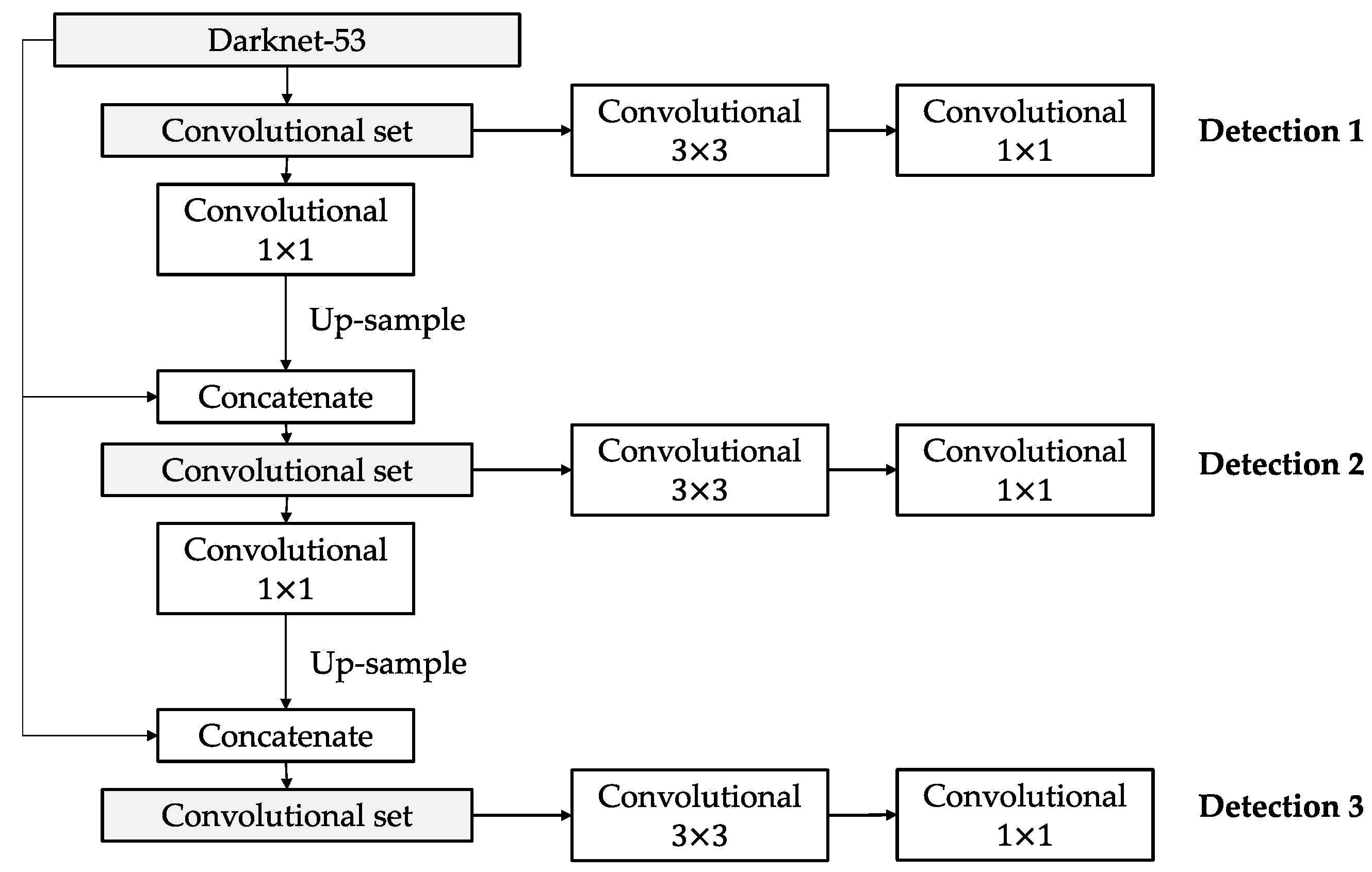
29] is a convolutional neural network for object localization, very fast for real-time applications, and has several versions. YOLOV3 architecture [
30] is composed of two main principal processes: a feature extractor called Darknet-53 and a convolutional method of the detection itself.
Figure 4 shows a block diagram for YOLOV3.
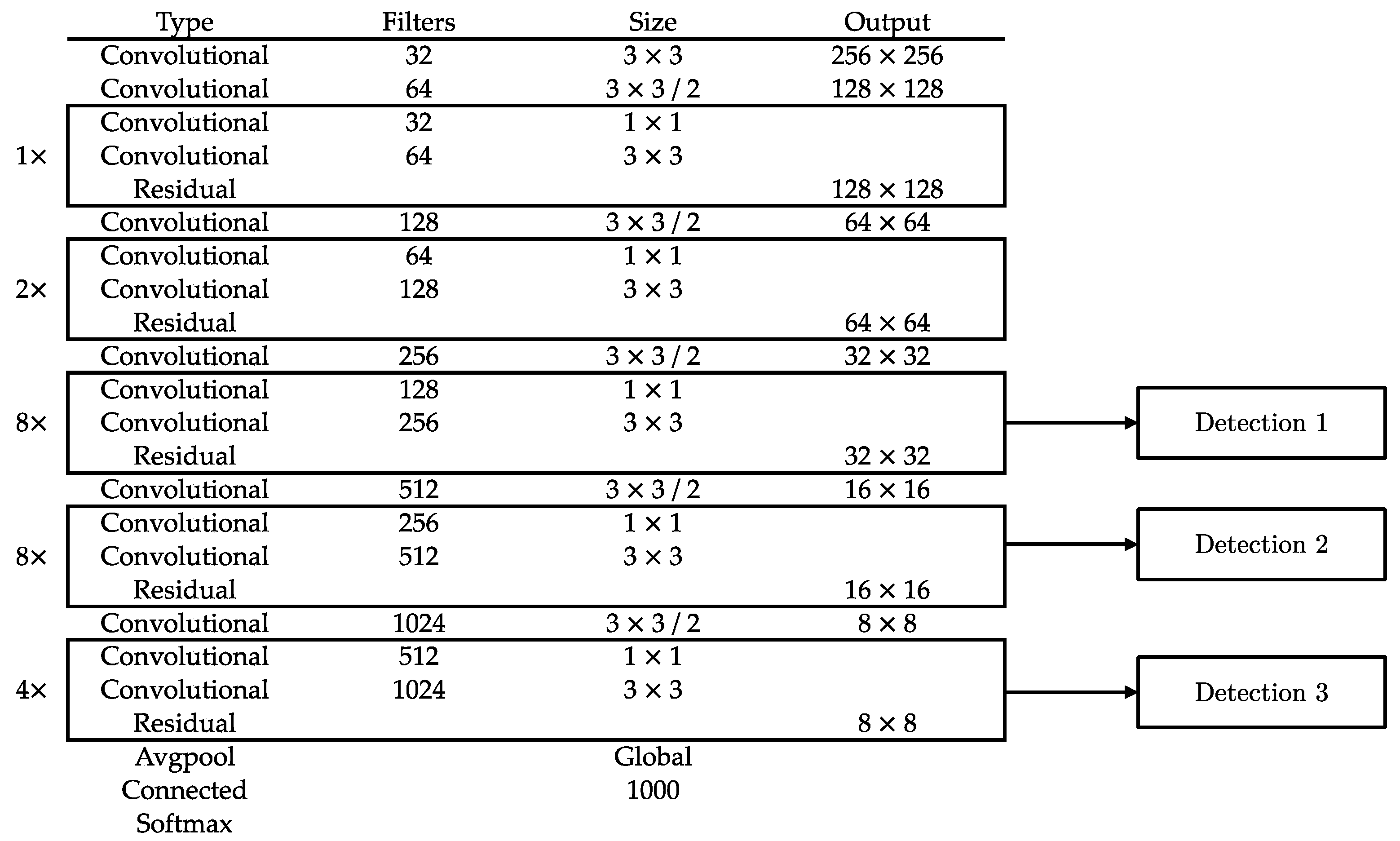
Figure 5 presents Darknet-53, which is a CNN with 53 layers of depth organized in five blocks of convolution layers, where each layer is a feature extractor. The last block of convolution layers contains the most important information obtained from this CNN, which is used to extract three detections of different scales.
A convolutional set is a process to change the dimensionality of the outputs of Darknet-53, which come from the last three blocks.
Figure 6 shows a convolutional set flow, which consists of a sequence of two convolutional filters: 1 × 1 and 3 × 3. A 1 × 1 convolutional filter allows one to obtain a feature map with a single dimension (WidthxHightx1). Usually, this filter is applied before an expansion filter: 3 × 3 convolution or 5 × 5 convolution.
YOLOV3 [
31] predicts a target value for each bounding box using logistic regression. The bounding box prediction consists of five components, as we see in Equation (4).
where
coordinates represent the center of the box concerning the location of the grid cell. These coordinates are normalized between 0 and 1. The confidence value indicates how likely it is that the box contains an object and how accurate the bounding box is. The pre-segmentation phase is a critical stage for obtaining accurate segmentation results. For comparison purposes, it should be included in the results stage.
3.3. Segmentation
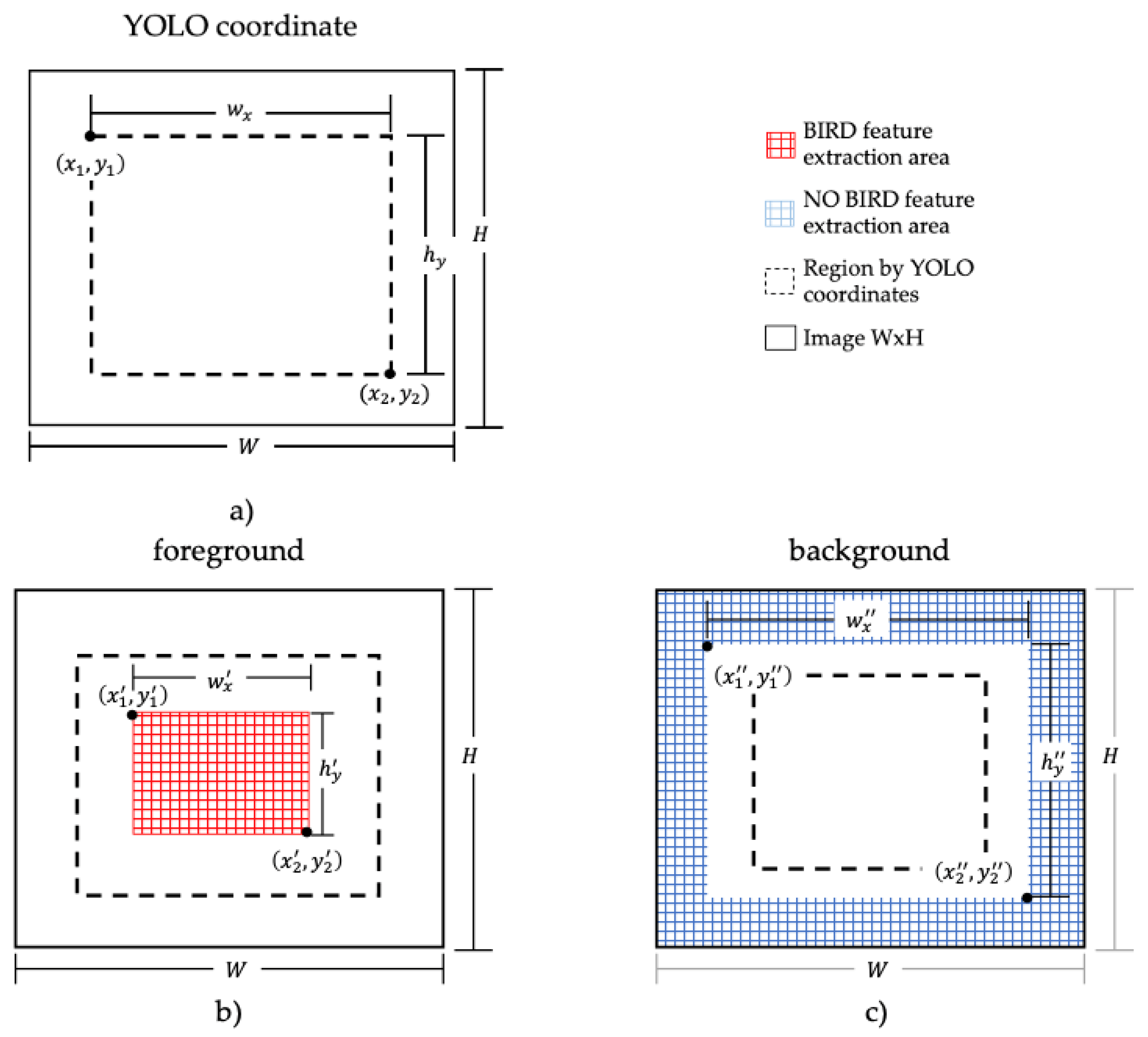
The segmentation phase aims to refine or adjust the region bounded by the coordinates from pre-segmentation to select a region of bird and no-bird.
Figure 7a shows an example of the segmentation phase proposed to delineate regions for birds and non-birds based on the coordinates obtained by pre-segmentation. The adjustment of the pre-segmentation coordinates is defined by two configurations:
Configuration 1: the pre-segmentation coordinates are reduced by 50%. Pixels within the range of Configuration 1 are classified as birds (
Figure 7b). The coordinates of Configuration 1 are described below:
Given a coordinate vector, Equation (4), with values
, the width of the region,
, and the height of the region,
, are determined, and the region of the bird is defined in Equations (5)–(7):
where (
and
are the coordinates from the origin
in the horizontal and vertical axis, respectively; (
and (
) are the new coordinates in the horizontal and vertical axis.
Configuration 2: pre-segmentation coordinates are increased by 20%. Pixels outside Configuration 2 are classified as non-birds,
Figure 7c. The coordinates of Configuration 1 are described below.
Given a coordinate vector, Equation (4), with values
, the width of the region
, and the height of the region
, are determined, and the region of the non-bird is defined in Equations (8)–(10) with the coordinates
and
:
where
and (
were previously defined for Equations (5)–(7).
The regions defined in Equations (5)–(10) are the pixels that are activated for feature extraction. The pixels between the bird and non-bird regions are not considered in the feature extraction phase. The label of a feature vector is assigned according to the region in which it is located.
3.4. Feature Extraction
Color features are extracted from 15 × 15 pixel regions, called super pixels, which represent a set of smoothed and enhanced images. The color features refer to the statistical behavior of the regions in each channel of the color models. The color models were selected according to the current state-of-the-art methods, and they are are HSI, CMYK, LAB, and XYZ. The variance and standard deviation are the features extracted for each channel.
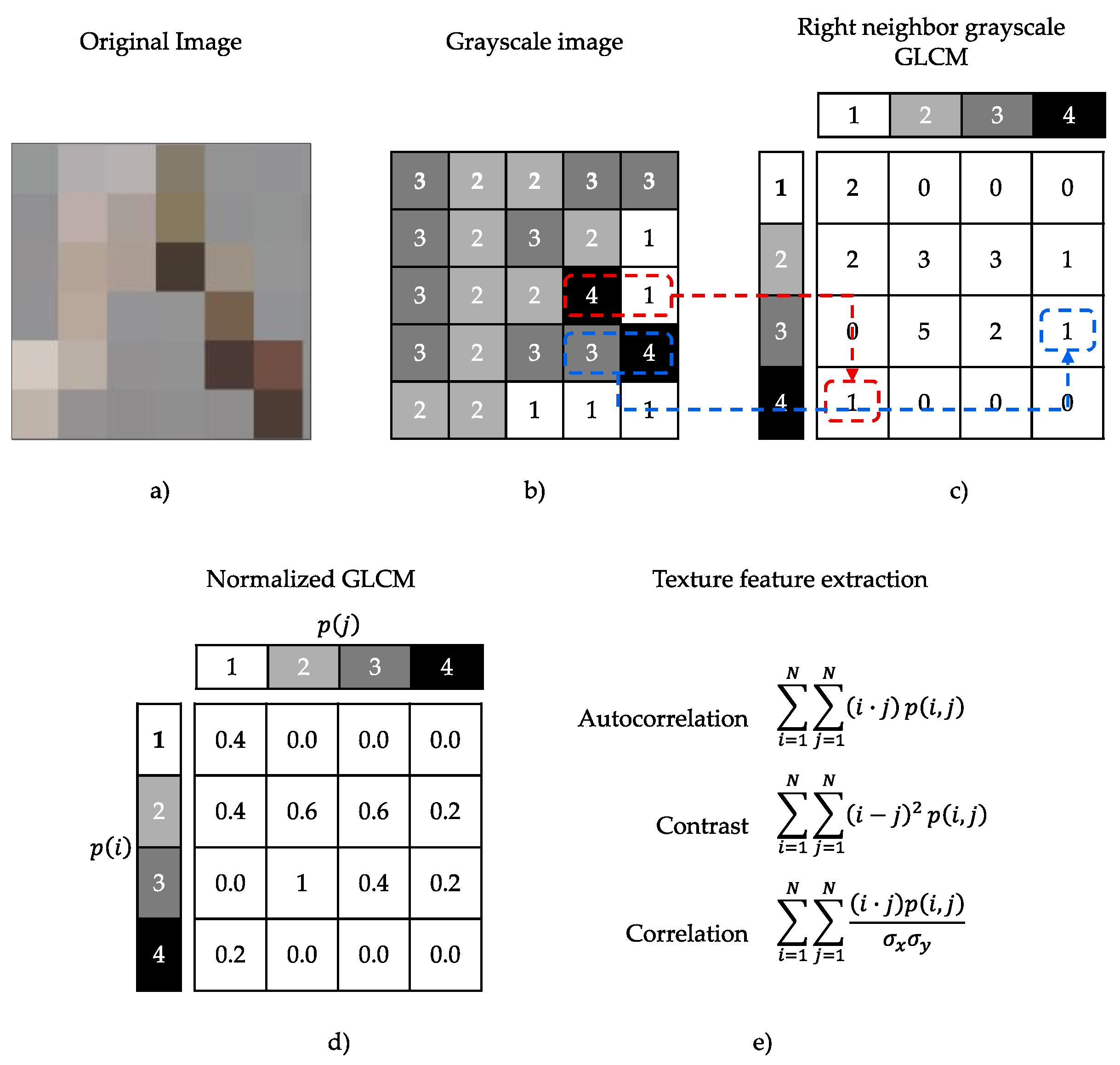
Haralick texture features [
32] are common texture descriptors in image analysis based on the concept that texture and hue are related. The features are determined using a correlation matrix of the intensity levels of an image, the gray-level co-occurrence matrix (GLCM). The number of gray levels in the image determines the size of the GLCM.
Figure 8 shows an example of how the GLCM is determined [
33].
GLCM starts with the transformation of an original image in RGB to a grayscale image, represented in
Figure 8a,b. In the second step, an occurrence matrix
is created, i.e., the values at the positions in
represent the number of times the gray level intensity value
is a neighbor of the gray level intensity value
, as we showed in
Figure 8c. After obtaining the occurrence matrix,
, the values
are normalized, as shown in
Figure 8d. Finally, the resulting matrix
is suitable for the application of the Haralick texture features (
Figure 8e).
Table 2 shows the notation of the variables involved in the calculation of the Haralick texture features. The first column represents the variable number; the second column shows the notation of the variables; and the third column describes the meaning of the notation.
Table 3 lists all the texture features used in this work. The first column represents the number of features; the second column is a name feature; in the third column, we have given an equation for the name feature.
3.5. Variable Feature Selector
The SA algorithm was proposed by Kirkpatrick in 1983 [
36]. SA represents the thermodynamic process of heating and cooling metal to increase its ductility and is an optimization method to find near-optimal solutions to non-deterministic polynomial-time hardness (NP-hardness) combinatorial problems [
37].
According to related work, the PCA technique is often used as a selector of relevant variables. This technique consists of describing the data in terms of new variables, called components. The components are ordered according to their explained variance, which represents the percentage of retention of the original information. However, each component is composed of a linear combination of all the original variables. Therefore, it can be said that PCA is a dimensionality reducer and not a variable selection method.
To solve the problem, a hybrid algorithm based on the simulated annealing (SA) technique and principal component analysis (PCA) was developed, which is called SA-PCA. SA-PCA has, as its solution, a binary vector with a length of 43, which is the number of descriptors that color and texture present in this work. The initial solution is established by PCA from the percentage contribution of the component variables, with the highest percentage of variance being explained.
Figure 9 shows an example of the representation of the initial solution for this work. The values 0 and 1 indicate whether a variable has been selected.
The definition of the SA-PCA parameters was subject to a tuning process [
37], which is discussed in more detail in
Section 4.4. Algorithm 1 shows the proposed SA-PCA algorithm, which is based on Kirkpatrick simulated annealing [
36]. First, lines 2 to 5 define the initial solution,
, and the objective function,
, which is associated with this solution. It is defined as the best solution found so far. Line 6 verifies that the best solution found so far has reached the minimum value.
SA-PCA is defined with two principal cycles (lines 7 and 8). Here, it is traditionally checked whether the initial temperature,
, has reached the final temperature,
, and whether the metropolis cycle has reached its maximum length,
, or if there is a state of convergence. The temperature,
, is to be adjusted by the parameter
, line 29. The inner cycle performs a search for a new solution,
, until a stochastic equilibrium,
, is reached at each low temperature by the parameter β.
is adjusted by parameter
in line 30. This algorithm allows the acceptance of bad solutions by the Boltzmann acceptance criterion in line 25.
| Algorithm 1 SA-PCA based on Kirkpatrick [36]. |
| | function SimulatedAnnealing |
| 1: | |
| 2: | |
| 3: | |
| 4: | |
| 5: | if then |
| 6: | while |
| 7: | while |
| 8: | |
| 9: | |
| 10: | |
| 11: | if |
| 12: | converge |
| 13: | end if |
| 14: | if(converge(metropoly)) |
| 15: | converge |
| 16: | end if |
| 17: | if |
| 18: | |
| 19: | |
| 20: | if |
| 21: | |
| 22: | |
| 23: | endif |
| 24: | elseif |
| 25: | |
| 26: | |
| 27: | endif |
| 28: | |
| 29: | |
| 30: | endwhile |
| 31: | if |
| 32: | if(converge(Temp)) |
| 33: | converge |
| 34: | endif |
| 35: | endif |
| 36: | endwhile |
| 37: | return |
| 38: |
endif |
| 39: | endfunction |
The SA-PCA algorithm has a perturbation phase, called
, which includes a roulette method with the purpose of increasing the probability of selection on those variables that have been part of good solutions in the past cycles (line 9). The acceptance criterion of a solution is given by the change in the value of the objective function between the actual solution,
, and the new solution,
, i.e.,
, where it is accepted if
, as seen in lines 11, 18 to 24. Otherwise, the Boltzmann-Gibbs distribution [
38], which is a decision or probability mechanism, and it is applied to determine if the bad solution is randomly accepted.
The convergence of the algorithm is defined in two cases of stable states: reaching the minimum value of the objective function, as well as stagnation. Stagnation is defined by successive repetitions of the value of the objective function of the new solution, , and the parameter . The convergence criterion in lines 33–35 means that convergence exists if the initial temperature is within 5% of the final temperature .
3.6. Classification
A random forest (RF) is an algorithm usually used for classification, which is composed of several decision tree classifiers, and it uses the average performance of the ensemble of classifiers to improve prediction accuracy, with the goal of optimizing the ensemble. Since the individual trees are randomly perturbed, the forest benefits from a wider exploration of the space of all possible predictors in the tree, which, in practice, result in better predictive performance [
39]. The most important aspects to consider in a RF are the number of decision trees in forest,
, the function to measure the quality of the prediction, and the maximum depth of the decision trees. A decision tree with
leaves divides the feature space into
regions,
,
[
40]. For each tree, the prediction function
is defined as:
where
is the number of regions in the feature space,
is a region appropriate to
, and
is a constant suitable to
in Equation (12). The hyperparameters of the classifier RF are discussed in more detail in
Section 4.3.
5. Results
We test our PSEV-BF methodology with a dataset from the COCO database. We evaluate our proposed methodology with APIoU’s mean semantic segmentation metrics for medium and large objects. In this section, we show the results obtained in the tuning phase and the selection of relevant variables for SA, as well as the performance of the model’s pre-segmentation and classification processes.
In the study of the better model, two distinct phases in computer vision were implemented and tested. The first phase, pre-segmentation, was a CNN architecture presented in
Section 3.2, consisting of locating the regions where ROI is found; YOLOV3 was used for this purpose. The coordinates provided by YOLOV3 allow the determination of the region where the object of interest could be located, which is performed during the segmentation phase.
We used the simulated annealing (SA) algorithm as a selector for relevant variables to improve the training phase in the classification process. SA-PCA used a random forest classifier. SA configures the initial solution using the variables obtained by PCA. It also uses a perturbation method using a roulette wheel. In
Table 7, we observe the solutions of SA-PCA that were proposed. The first column indicates the number of runs, the second column shows the number of features selected in each run, and the third column is the objective function associated with the number of variables selected. The choice of a solution, i.e., a set of variables, obtained by the SA-PCA, is defined by the size of the solution and the objective function, the latter being the most important. Thus,
Table 7 shows that, by using 14 variables, an objective function with a lower error rate is obtained. Therefore, these characteristics are used as relevant variables.
The classification performances for two groups of bird sizes are given in
Table 4. We observe the comparative performance of the proposed methodology with different configurations: Methodology 1 (M1), Methodology 2 (M2), and Methodology 3 (M3). The M1 configuration applies the traditional processes of pre-processing, classification, evaluation, and a superpixel technique. M2 involves the same traditional process but does not use superpixels, although a variable selection method is implemented. M3 only implements a pre-segmentation phase with YOLOV3. Additionally, finally, our proposal PSEV-BF includes all the configurations proposed in this work. It is important to clarify that all methodologies use pre-segmentation with YOLOV3 for comparison purposes.
In
Table 8, the first column indicates the size of the birds used: large or medium. The second column lists the different methodologies, labeled M1, M2, M3, and our PSEV-BF. The third and fourth columns indicate, with ✓, whether the superpixel technique is used in the pre-segmentation, segmentation, or enhanced feature phase, and it indicates ✗ otherwise. Finally, the last two columns are the results from APIoU with two thresholds: 0.5 to 0.95 and 0.75 to 0.95.
In
Table 8, the results show that the proposed PSEV-BF methodology for large objects has values around 50% for the APIoU metric and 80% for the APIoU
75 metric. On the other hand, medium-sized objects have values around 36% for the APIoU metric and 80% for the APIoU
75 metric for the M2 and M1 methodologies. However, M1 for medium-sized objects did not obtain images with a higher value than the 75% threshold of the APIOU
75 metric, and they were not calculated. The average processing times obtained by the PSEV-BF in large and medium objects were 78.03 and 3.07 s, respectively. Additionally, the processing time for the M1 methodology for large objects was 90.09 s, and, for medium objects, it was 9.01. In the case of M2 and M3 methodologies, the superpixel is not included, and the time processing is not reported because the time exceeds the maximum time allowed for each image.
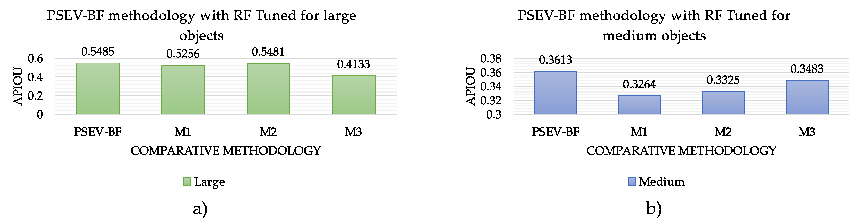
In
Figure 10, we present the performance of the different configurations of the proposed method based on the APIoU metric with a threshold starting at 0.5 for large and medium size objects and reaching values around 50%. In
Figure 10a, we show that our proposal achieves a performance of 54% accuracy for large objects, with a difference of about 12% with the M3 methodology, which achieves the lowest accuracy. The M2 and M3 methodologies obtained APIoU values very close to those of the PSEV-BF methodology. They are involved in at least two of the proposed processes: superpixel and pre-segmentation.
In
Figure 10b, we observed that the PSEV-BF achieves a performance of 36% accuracy for medium size objects, with a difference of about 4% from the M1 methodology, which achieves the lowest accuracy. The M3 methodology shows values close to those of the proposed method, and these are involved in pre-segmentation.
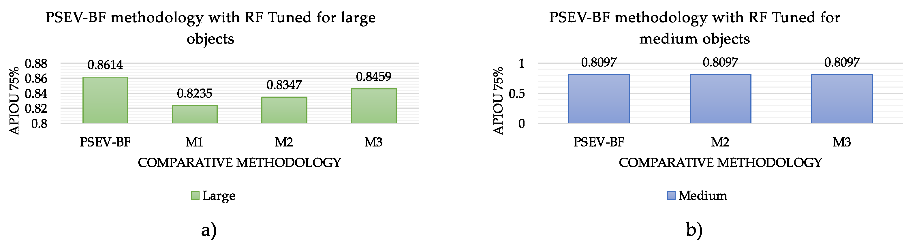
In
Figure 11, we can observe the performance of the different configurations of the proposed method based on the APIoU metric, with a threshold starting at 0.75 for large- and medium-sized objects and reaching values around 80%.
Figure 11a shows that our proposal achieves a performance of 86% accuracy for large objects, with a difference of about 4% with the M1 methodology, which achieves the lowest accuracy. The M3 methodology shows values very close to those of the PSEV-BF methodology; these are involved in at least two of the proposed processes: superpixel and pre-segmentation.
In
Figure 11, we present the performance of the methods for medium- and large-sized objects, considering those images that reach a threshold equal or greater than 75% (
). In
Figure 11b, we observe that PSEV-BF methodology, as well as M2 and M3, achieve an accuracy of 80% for medium-sized objects. On the contrary, the methodology M1 fails to obtain an accuracy above a threshold of 75%.
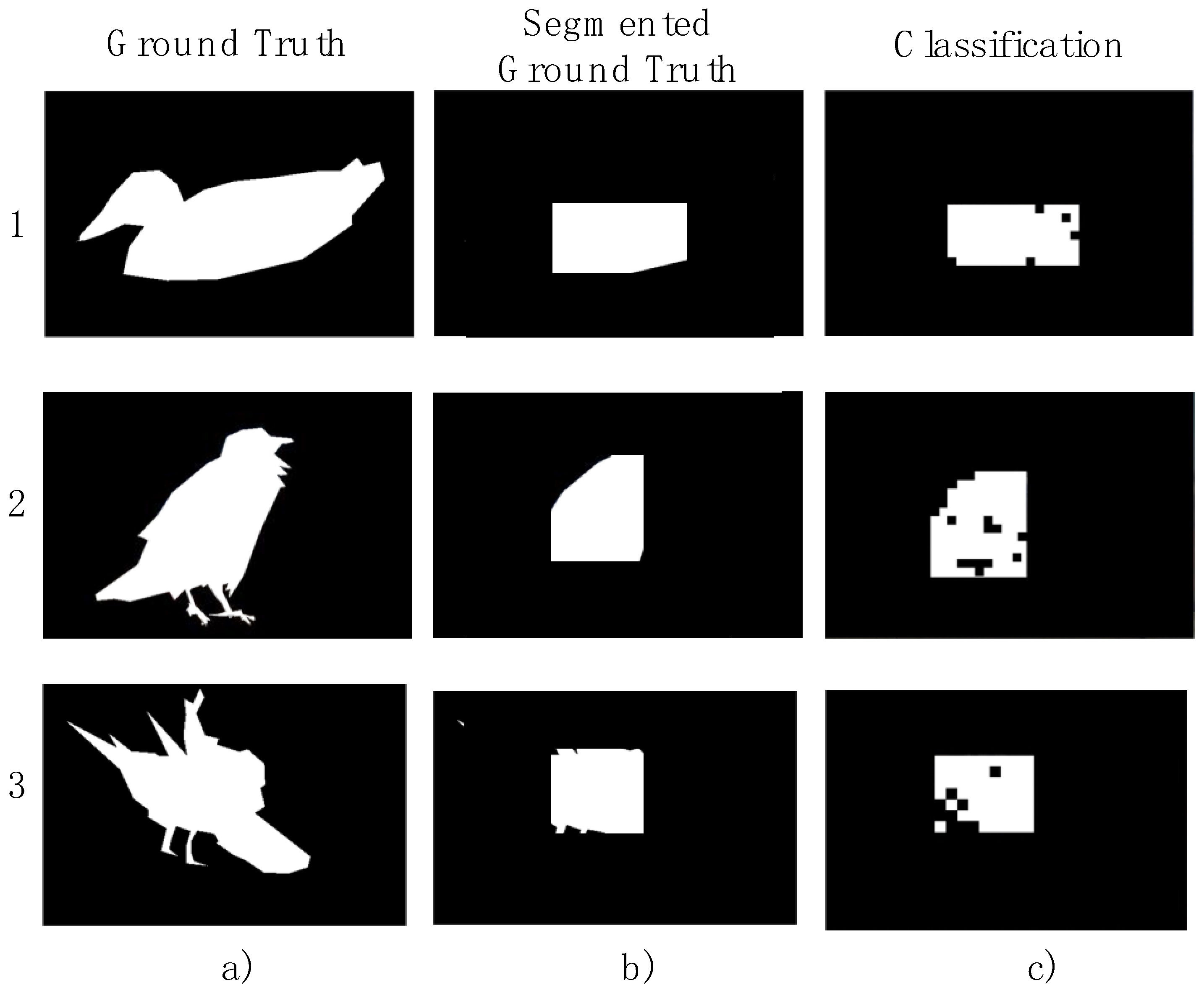
Figure 12 shows some examples of objects with large sizes processed.
Figure 12a shows the images segmented by COCO;
Figure 12b shows the adaptation resulting from the segmentation phase. Finally,
Figure 12c shows some of the cases obtained using the PSEV-BF methodology. We observe that the pixels corresponding to non-birds (black blocks) are part of the background. Likewise, about 86% of the pixels corresponding to birds were correctly classified.
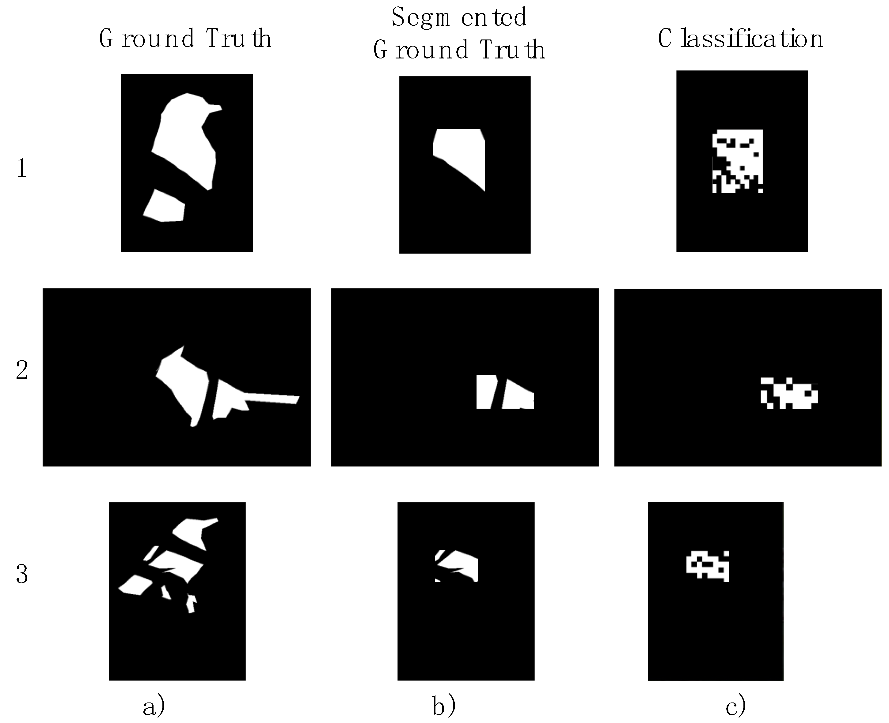
Figure 13 shows some examples of objects with large sizes that are processed with occlusion.
Figure 13a shows that the white pixels correspond to birds, and the black pixels correspond to non-birds (or wrongly classified pixels). Likewise, about 86% of the pixels corresponding to birds were correctly classified.
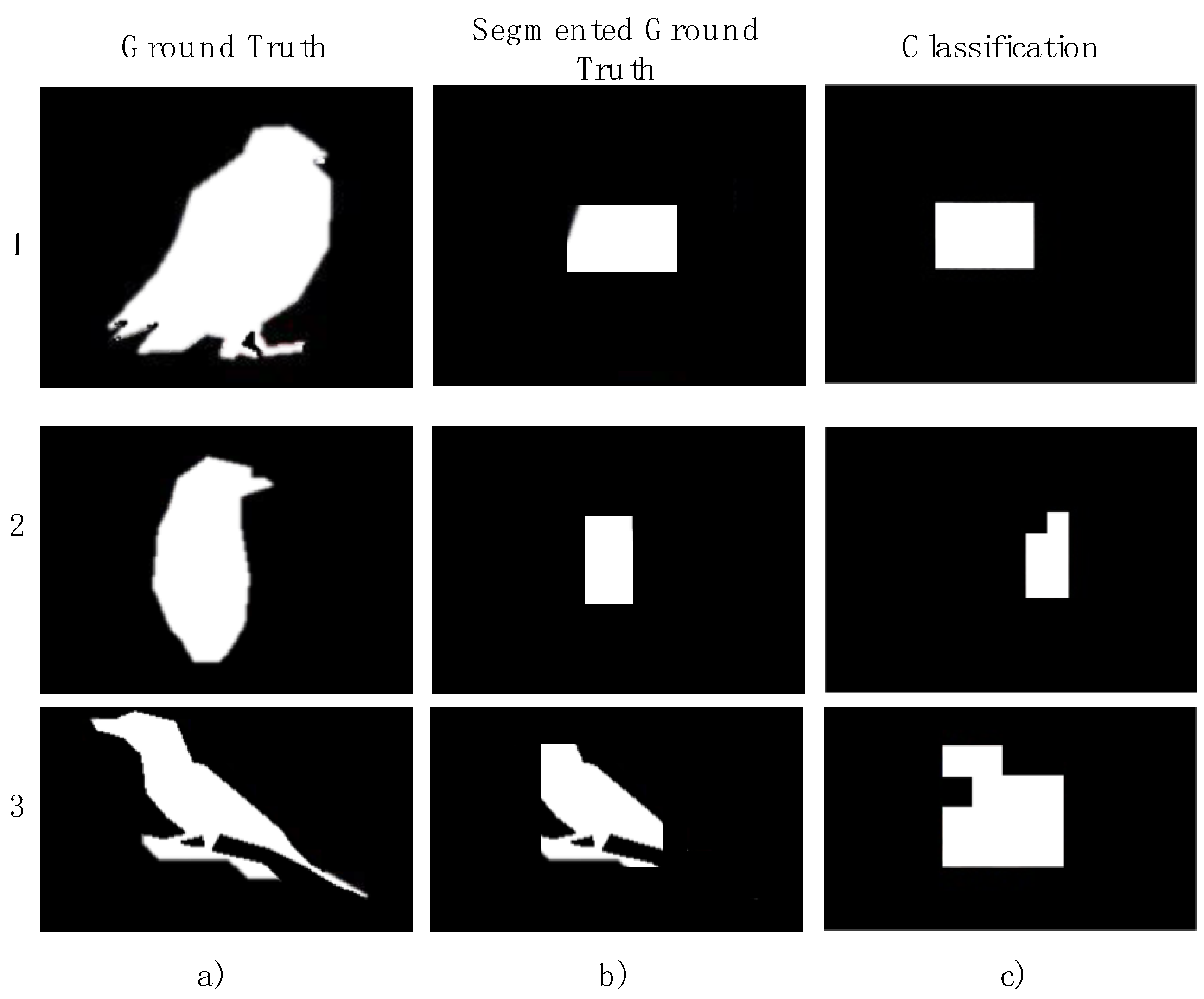
Figure 14 shows some examples of objects with medium sizes processed by the PSEV-BF methodology. We observe, in the last column, the pixels corresponding to birds (white pixels) which were correctly classified in the first row.
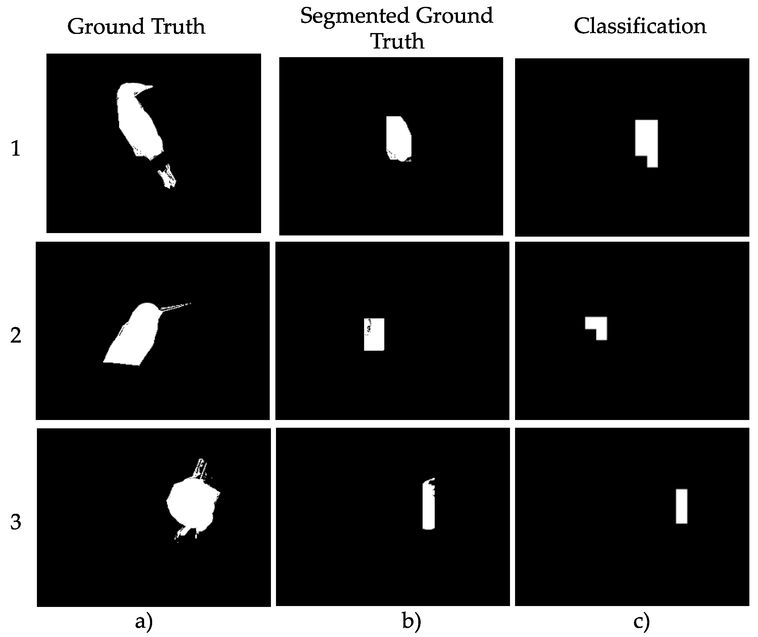
Finally,
Figure 15 shows some examples of objects with medium sizes processed with occlusion by the PSEV-BF methodology. We observe, in the last column, that the pixels corresponding to birds were correctly classified.
6. Conclusions
In this paper, we presented a bird detection and classification methodology called PSEV-BF (pre-segmentation and enhanced variables for bird features), which uses pre-segmentation and a simulated annealing algorithm with principal component analysis called SA-PCA, proposed to enhance variables. PSEV-BF incorporates a new methodology compared to modern methods. Moreover, it can be applied to images with occlusions and uncontrolled environments.
The methodology of PSEV- BF consists of the phases of preprocessing, pre-segmentation, segmentation, feature extraction, relevant variables selection, and classification. Preprocessing includes histogram equalization and Gaussian filtering for image enhancement and smoothing. For pre-segmentation, a CNN detection technique, YOLOV3, was used to provide a vector of coordinates. The coordinates delineate a region that has a high probability of belonging to a bird.
Segmentation refines the coordinates obtained from pre-segmentation by redefining the given region. The inner region of the coordinates is reduced by 50% and catalogued as foreground pixels. The outer region of the coordinates is increased by 20% and cataloged as background pixels. A superpixel technique was used in feature extraction to obtain a 43-feature vector with color and texture. The superpixel technique covers an area of 15 × 15 pixels.
We compare our methodology with the traditional methodology. The methodology was tested with bird category images from the COCO database. The images were classified according to the size of the desired object: large and medium. A total of 193 images were used for training and validation of the classifier, and 70 images were used for testing. The test images are divided into large and medium groups, which correspond to 35 images per group. A total of 16,988 feature vectors were used as samples for the training and validation of the random forest classifier.
PSEV-BF was compared with the M1, M2, and M3 methodologies. These methodologies differ in configuration from the proposed methodology. For large objects, PSEV-BF and M2 show values with an approximate accuracy of 54% with the APIoU metric, whereas M2 does not have the superpixel phase. First, M1 and M2 use at least two of the proposed methods in the methodology. However, M3 does not use the proposed phases, resulting in 41% accuracy of the APIoU metric, which is the lowest value among the compared methodologies. Secondly, M2 does not use the superpixel method, which leads to a very similar accuracy value compared to PSEV-BF, while M1 has a difference of 2% compared to M2. We can say that using the proposed processes for large objects improves the accuracy of the methodology.
For objects classified as medium size, the methodology of PSEV-BF shows values with an approximate accuracy of 36% of the APIoU metric. First, M1 shows 32% accuracy, which is the lowest value among the compared methodologies. This means that the effects are very large when segmentation and enhanced variables are not used. PSEV-BF and M1 differ by 4%, and the difference is due to the use of a superpixel method. We find that, in PSEV-BF in medium-sized objects, prediction accuracy is improved.
This paper presents a methodology for pre-segmentation, the variable selection method, and feature extraction employing superpixels. Once the methodology is tuned, it can be used to solve object identification problems, for example, classification by type of bird or other objects faster than traditional methods.
For future work, we propose using similar techniques for supervised image segmentation. PSEV-BF was not designed for recognizing species of birds. We plan to incorporate other strategies for pre-segmentation, enhanced feature variables, and classification for recognizing different species.


 ,
, 


