Calculation of the Free Energy of the Ising Model on a Cayley Tree via the Self-Similarity Method

Abstract

In this study, an interactive Ising model having the nearest and prolonged next-nearest neighbors defined on a Cayley tree is considered. Inspired by the results obtained for the one-dimensional Ising model, we will construct the partition function and then calculate the free energy of the Ising model having the prolonged next nearest and nearest neighbor interactions and external field on a two-order Cayley tree using the self-similarity of the semi-infinite Cayley tree. The phase transition problem for the Ising system is investigated under the given conditions.

1. Introduction

For a long time, the Cayley tree (shortly, CT) and the Bethe lattice (shortly, BL) have been used extensively in many branches such as statistical physics [1], statistical mechanics [2,3], and mathematics [4,5]. Basically, the main features that make these two graphs important are that the operations on them are incredibly easy compared to realistic lattices such as ${\mathbb{Z}}^d$ ($d\ge 2$) [3]. In particular, the self-similarity feature of the semi-infinite CT provides great convenience in examining important issues such as the Gibbs measures and the free energy (see [6,7,8,9,10] for details). A limited number of the total turns in a CT are located at the boundary. The CT is a substantially in-homogeneous system as a result, and its characteristics frequently differ greatly from those of a typical finite-dimensional issue [1]. We refer the reader to Ostilli’s work [6] to understand the relationships between the CT and the BL.

Deriving the recursive equations characterizing the Gibbs measure for the lattice models on the CT can be done in a number of different ways. One method is based on Markov random field (MRF) characteristics on BL [2,11,12]. The recursive equations for the partition functions are the foundation of another strategy (see [11]). Naturally, the same equation results from both methods [4,5]. The second strategy works better with models that have the competing interactions. The second method is also called the cavity method [1,6]. The cavity method is also known as the self-similarity method [6]. Mezard and Parisi [1] suggested a generic, non-perturbative solution to the BL spin glass issue using the cavity approach. The cavity method in computer science is called belief-propagation (BP). The Bethe approximation in statistical physics and the BP method are closely related concepts (see [13] for details).

In Ref. [10], Gandolfo et al. provide some explicit equations for the free energies associated with boundary conditions for the Ising model on the CT. The author of [14] presents a practical method for providing some formulas for the free energy and entropy for a given Ising model using the Kolmogorov consistency theorem (KCM) taking into account some boundary conditions. The formula for the free energy connected to the translation-invariant Gibbs measures, which enables the calculation of the related entropy, was obtained by the authors as an illustration of the presented technique in [15].

To the best of the author’s knowledge, the free energy formulas of the lattice models on the CT were calculated using the KCM [4,10,14,15]. Recently, the Gibbs measures of lattice models on CT-like lattices and the consequent phase transition problem have been investigated using the KCM (see [16,17]). The Gibbs measures for the q-state Potts model on the CT were determined using the self-similarity method [11,18]. In this study, we will derive the free energy formula for the model using the self-similarity of the semi-infinite CT. Thanks to this method, we will obtain this formula without constructing Gibbs measures for the given boundary condition.

As mentioned above, in order to investigate many quantities in the statistical mechanics, it is necessary to derive the partition function for the lattice model under consideration. Few studies have been done recently using the KCM to calculate the free energy of the Ising model given on the CT [4,14,19]. In this present work, we will obtain the partition function by taking into account the self-similarity method to calculate the free energy of the Ising model defined on the CT. Considering the fractal structure of the semi-infinite CT, the iterative method contributes to the easy solution of most difficult problems. Here we will use the iteration approach to derive the partial partition functions. We will investigate the existence of the phase transition for the Ising system under the given conditions.

2. Preliminaries and Main Definitions

In this section, we will give some concepts that have been defined in different studies before.

2.1. The Cayley Tree

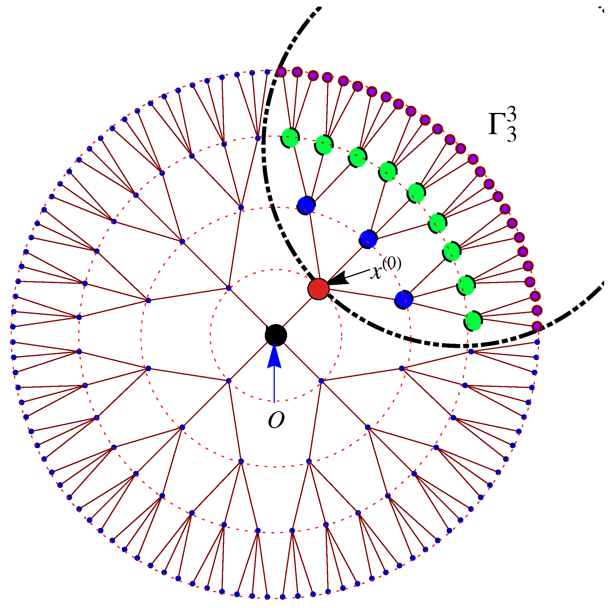
The CT is straightforward linked undirected graph without cycles. It has a fractal structure. Let us denote a CT of order k having n shells by $G_{k,n}$. Let O be the root vertex, we use k edges to connect O with k new vertices. This initial set of k vertices makes up the shell $n=1$ of the CT and we denote this set by $W_1$. Then, with $n\ge 2$, k vertices are connected with new k edges to each vertex in the $(n-1)$th shell to form the nth shell. Thus, these added vertices form the set $W_n$ of vertices located on nth shell of the the CT $G_{k,n}$. The structure of the CT $G_{4,4}$ with the root vertex O is shown in Figure 1 (see [6,8,20] for details).

Let ${\mathrm{\Gamma }}^k=(V,L)$ denote a semi-infinite CT of order k ($k\ge 1$) having the root $x^{\left(0\right)}$. Here V is the set of vertices and L is the set of edges. While the root vertex $x^{\left(0\right)}$ of the semi-infinite CT ${\mathrm{\Gamma }}^k$ of order k is connected with only k vertices only with one edge, all other vertices of the tree are connected with $(k+1)$ vertices by only one edge (see [4] for details).

The distance $d(x,y),x,y\in V$, on the CT, is the length of the shortest path from x to y. In other words, $d(x,y)$ is the number of edges in the shortest distance connecting the x and y vertices. For $n=1,2,\cdots$, $S\left(x\right)=\left\{y\in W_n:d(x,y)=1\right\}$ is the set of direct successors of $x\in W_{n-1}$, where

$$W_n=\left\{x\in V\mid d(x,x^{\left(0\right)})=n\right\}.$$

Throughout the paper, we will denote the semi-finite CT of order k with n shells by ${\mathrm{\Gamma }}_n^k=(V_n,L_n)$, where we have

$$V_n=\bigcup _{m=0}^n{W}_m,L_n=\left\{\ell =<x,y>\in L\mid x,y\in V_n\right\}.$$

For example, in Figure 1, the root of the tree ${\mathrm{\Gamma }}_3^3$ is represented by the vertex that is red and labeled with $x^{\left(0\right)}$. In Figure 1, one can see that each vertex in ${\mathrm{\Gamma }}_3^3$ has 4 edges except for the root vertex $x^{\left(0\right)}$ having 3 edges. For the sake of completeness, note that Figure 1 and the explanations for constructing a semi-finite CT are borrowed from Ref. [8].

In this study, we will consider two kinds of neighborhood interactions. Let us now give their definition.

Definition 1.

1. For $x,y\in V$, the vertices x and y are called nearest-neighbors (NN) if there exists a single edge $\langle x,y\rangle \in L$ connecting them.

2. The vertices x and y are called prolonged next-nearest-neighbors (PNNN) if $d(x,x^{\left(0\right)})\ne d(y,x^{\left(0\right)})$ and $d(x,y)=2$ it is denoted by $\rangle x,y\langle$, where $x^{\left(0\right)}$ is the root of the CT ${\mathrm{\Gamma }}^k$.

2.2. Ising Model

In this paper, we will consider the Ising model on the second-order CT defined by the Hamiltonian

$$\begin{array}{ccc}\hfill H\left(\sigma \right)& =& -J\sum _{\langle x,y\rangle }\sigma \left(x\right)\sigma \left(y\right)-J_p\sum _{\rangle x,y\langle }\sigma \left(x\right)\sigma \left(y\right)-\sum _{x\in V}{h}_x\sigma \left(x\right),\hfill \end{array}$$

(1)

where the first term is the energy of each of the bonds between nearest neighboring sites, and the second term is the energy of each of the bonds between prolonged next-nearest neighboring sites, and the third is the energy of each of the sites.

Let U be a finite subset of V. We shall indicate the restriction of $\sigma$ to U by $\sigma \left(U\right)$. Consider the fixed boundary configuration $\overline{\sigma }(V\backslash U)$. Under the boundary condition $\overline{\sigma }(V\backslash U)$, the total energy of $\sigma \left(U\right)$ is defined as

$$\begin{array}{ccc}\hfill H_U\left(\sigma \left(U\right)\right|\overline{\sigma }(V\backslash U))& =& -J\left(\sum _{\langle x,y\rangle :x,y\in U}\sigma \left(x\right)\sigma \left(y\right)+\sum _{\langle x,y\rangle :x\in U,y\notin U}\sigma \left(x\right)\sigma \left(y\right)\right)\hfill \\ \hfill & & -J_p\left(\sum _{\rangle x,y\langle :x,y\in U}\sigma \left(x\right)\sigma \left(y\right)+\sum _{\rangle x,y\langle :x\in U,y\notin U}\sigma \left(x\right)\sigma \left(y\right)\right)-\sum _{x\in U}{h}_x\sigma \left(x\right).\hfill \end{array}$$

(2)

Considering $\overline{\sigma }(V\backslash U)$, we define the partition function $Z_U\left(\overline{\sigma }(V\backslash U)\right)$ in volume U by

$$\begin{array}{c}\hfill Z_U\left(\overline{\sigma }(V\backslash U)\right)=\sum _{\sigma \left(U\right)\in {\mathrm{\Phi }}^U}{e}^{-\beta H_U\left(\sigma \left(U\right)\right|\overline{\sigma }(V\backslash U))},\end{array}$$

(3)

where $\beta =\frac{1}{T}$ is the inverse temperature.

For the sake of simplicity, we shall refer to $Z_{V_n}$ and the configuration $\sigma \left(V_n\right)$ in volume $V_n$ as ${\sigma }_n$ and $Z^{\left(n\right)}$, respectively. The total partition function $Z^{\left(n\right)}$ may be broken down into the summands:

$$Z^{\left(n\right)}=\sum _{i\in \mathrm{\Phi }}{Z}_i^{\left(n\right)},$$

(4)

where

$$Z_i^{\left(n\right)}=\sum _{{\sigma }_n\in {\mathrm{\Phi }}^{V_n}:\sigma \left(x^{\left(0\right)}\right)=i}exp(-\beta H_{V_n}\left({\sigma }_n\right|\overline{\sigma }(V\backslash V_n)).$$

In order to fundamentally simplify the problem, Ganikhodjaev et al. [11] suggested a procedure for calculating the partial partition functions of 3-state Potts model of order two utilizing the self-similarity of the semi-infinite CT. Ganikhodjaev et al. [11] computed the partial partition functions as

$$Z_{i_0}^{\left(n\right)}=\sum _{\eta \in {\{1,2,3\}}^{B_1\left(x^{\left(0\right)}\right)}}exp\left(-\beta H\left(\eta \right)+\beta h{\delta }_{1i_0}\right)Z_{i_1}^{(n-1)}{Z}_{i_2}^{(n-1)},$$

where ${\delta }_{1i_0}$ is a Kronecker’s symbol, H is a Hamiltonian of the Potts model having two competing binary interactions, and h is an external field (also see [21] for details).

3. Partition Function and Free Energy

In this section, we will first construct the partition function for the Ising model using the self-similarity approach, and then calculate the free energy of the model with the help of the partition function. Here, the iterative approach will be considered.

The Self-Similarity Approach

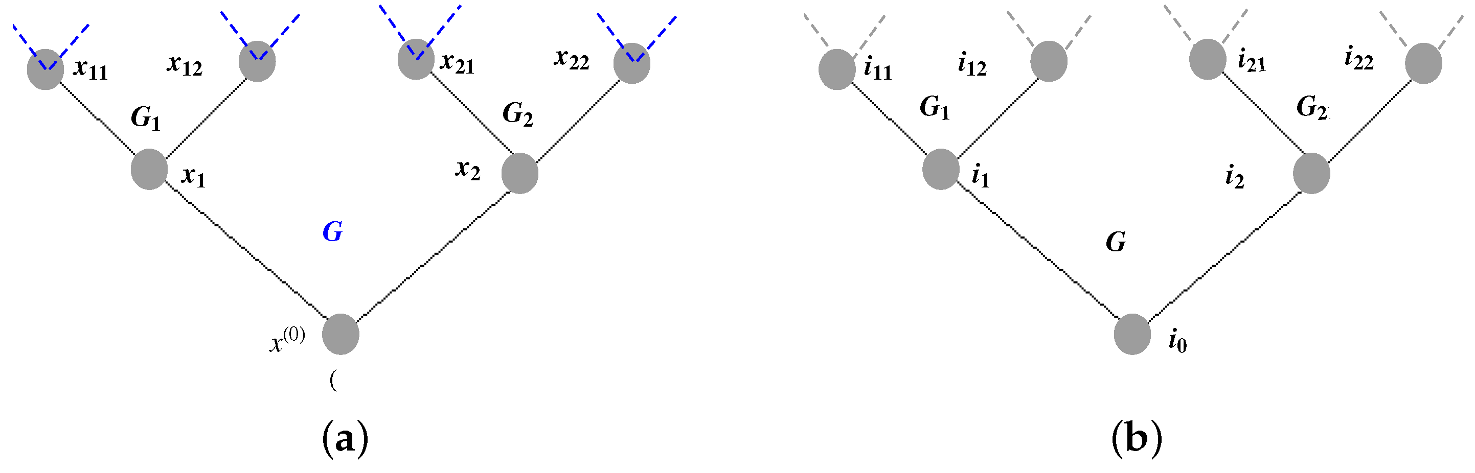
Let us consider a CT of order two having the root vertex $x^{\left(0\right)}$ (see Figure 2a). Two edges pointing at the vertices $x_1$ and $x_2$ emerge from the root vertex $x^{\left(0\right)}$. If we consider the lattice G as infinite, then we obtain two infinite subgraphs $G_1$ and $G_2$ which are equivalent to each other. Thus, we obtain the self-similarity $G=G_1=G_2$ (see [6] for details).

We define a semi-ball with radius 2 and the center $x^{\left(0\right)}$ by

$$B_2\left(x^{\left(0\right)}\right):=\left\{x^{\left(0\right)},x_1,x_2,x_{11},x_{12},x_{21},x_{22}\right\}$$

(see Figure 2a), and denote the set of configurations to be placed on the semi-ball $B_2\left(x^{\left(0\right)}\right)$ by

$${\mathrm{\Phi }}^{B_2\left(x^{\left(0\right)}\right)}=\{i_0,i_1,i_2,i_{11},i_{12},i_{21},i_{22}\},$$

where $\mathrm{\Phi }=\{-1,+1\}$ (see Figure 2b).

Note that in this paper we assume $h_x=h$ for all $x\in V$. Taking into account the Hamiltonian (1), we define the energy of a configuration on the semi-ball $B_2\left(x^{\left(0\right)}\right)$ by

$$\begin{array}{ccc}\hfill E\left(\sigma \left(B_2\left(x^{\left(0\right)}\right)\right)\right)& =& -\beta J_p\sigma \left(x^{\left(0\right)}\right)\sum _{a,b\in \{1,2\}}\sigma \left(x_{ab}\right)-\beta J\sigma \left(x^{\left(0\right)}\right)\left(\sigma \left(x_1\right)+\sigma \left(x_2\right)\right)\hfill \\ \hfill & & -\beta J\sum _{a=1}^2(\sigma \left(x_a\right)(\sigma \left(x_{a1}\right)+\sigma \left(x_{a2}\right))-\sum _{a,b\in \{1,2\}}h\sigma \left(x_{ab}\right),\hfill \end{array}$$

(5)

where the configurations $\sigma \left(B_2\left(x^{\left(0\right)}\right)\right)\in {\mathrm{\Phi }}^{B_2\left(x^{\left(0\right)}\right)}$.

Let us consider Figure 2b. We can calculate the full energy of the configurations on the semi-ball $B_2\left(x^{\left(0\right)}\right)$ with the help of the following function

$$\begin{array}{c}\hfill E(i_0,i_1,i_2):=\sum _{i_{11}\in \mathrm{\Phi }}\sum _{i_{12}\in \mathrm{\Phi }}\sum _{i_{21}\in \mathrm{\Phi }}\sum _{i_{22}\in \mathrm{\Phi }}{e}^{\beta J(i_1(i_{11}+i_{12})+i_2(i_{21}+i_{22}))+\beta J_p{i}_0(i_{11}+i_{12}+i_{21}+i_{22})+\beta h(i_{11}+i_{12}+i_{21}+i_{22})}.\end{array}$$

(6)

It should be noted here that the expression $\beta J\sigma \left(x^{\left(0\right)}\right)\left(\sigma \left(x_1\right)+\sigma \left(x_2\right)\right)$ in Equation (5) is not taken into account in Equation (6). As is known, the structure of a semi-infinite CT constitutes a fractal. If $\beta J\sigma \left(x^{\left(0\right)}\right)\left(\sigma \left(x_1\right)+\sigma \left(x_2\right)\right)$ is taken into account in (6), in sequential calculations, the total energy between the nearest vertices on first two consecutive levels will be calculated twice. For example, in the first step, in addition to $\beta J\sigma \left(x^{\left(0\right)}\right)\left(\sigma \left(x_1\right)+\sigma \left(x_2\right)\right)$, the total energy between the nearest vertices of the $W_1$ and $W_2$ will also be calculated. When the second step is passed, both the total energy between the nearest vertices in $W_1$ and $W_2$ and the total energy between the nearest vertices in $W_2$ and $W_3$ will be calculated. However, in the first step, we have already calculated the total energy between the nearest vertices in $W_1$ and $W_2$. Ignoring $\beta J\sigma \left(x^{\left(0\right)}\right)\left(\sigma \left(x_1\right)+\sigma \left(x_2\right)\right)$ does not change the value of the total partition function. Therefore, we will consider Equation (6) in our future calculations.

Lemma 1.

Let us consider the Hamiltonian (1) and Equation (6), then we have

$$\begin{array}{c}\hfill \sum _{\eta \in {\mathrm{\Phi }}^{B_2\left(x^{\left(0\right)}\right)}}E\left(\eta \right)={\left(\frac{\left(1+{\theta }^2\right)+4\theta \phi u+{\phi }^2\left(1+{\theta }^2\right)u^2}{\theta \phi u}\right)}^2+{\left(\frac{\left(1+{\theta }^2\right)u^2+4\theta \phi u+{\phi }^2\left(1+{\theta }^2\right)}{\theta \phi u}\right)}^2.\end{array}$$

(7)

Proof. 

Let us calculate $E(i_0,i_1,i_2)$ values separately for $i_0,i_1,i_2\in \mathrm{\Phi }.$ Obviously, 8 different values are obtained here.

$$\begin{array}{c}\hfill \left\{\begin{array}{c}E(1,1,1)=e^{-4(h+J+J_p)\beta }{\left(1+e^{2(h+J+J_p)\beta }\right)}^4,\hfill \\ E(1,1,-1)=E(1,-1,1)=e^{-4(h+J+J_p)\beta }{\left(e^{2J\beta }+e^{2(h+J_p)\beta }\right)}^2{\left(1+e^{2(h+J+J_p)\beta }\right)}^2,\hfill \\ E(1,-1,-1)=e^{-4(h+J+J_p)\beta }{\left(e^{2J\beta }+e^{2(h+J_p)\beta }\right)}^4,\hfill \\ E(-1,1,1)=e^{-4(h+J+J_p)\beta }{\left(e^{2(h+J)\beta }+e^{2J_p\beta }\right)}^4,\hfill \\ E(-1,1,-1)=E(-1,-1,1)=e^{-4(h+J+J_p)\beta }{\left(e^{2(h+J)\beta }+e^{2J_p\beta }\right)}^2{\left(e^{2h\beta }+e^{2(J+J_p)\beta }\right)}^2,\hfill \\ E(-1,-1,-1)=e^{-4(h+J+J_p)\beta }{\left(e^{2h\beta }+e^{2(J+J_p)\beta }\right)}^4.\hfill \end{array}\right.\end{array}$$

(8)

For sake of brevity, let us do the variable substitution $\theta =e^{\frac{\beta J}{2}},\phi =e^{\frac{\beta J_p}{2}}$ and $u=e^{\frac{\beta h}{2}}$. From the equations given in (8), we obtain

$$\begin{array}{ccc}\hfill E(1,1,1)+2E(1,1,-1)+E(1,-1,-1)& =& {\left(\frac{\left(1+{\theta }^2\right)+4\theta \phi u+{\phi }^2\left(1+{\theta }^2\right)u^2}{\theta \phi u}\right)}^2,\hfill \end{array}$$

(9)

$$\begin{array}{ccc}\hfill E(-1,1,1)+2E(-1,1,-1)+E(-1,-1,-1)& =& {\left(\frac{\left(1+{\theta }^2\right)u^2+4\theta \phi u+{\phi }^2\left(1+{\theta }^2\right)}{\theta \phi u}\right)}^2.\hfill \end{array}$$

(10)

If we add Equations (9) and (10) side by side, we complete the proof of the lemma.  □

One of our main results is the following theorem.

Theorem 1.

Fix a finite volume $V_n\subset V$. Then on $V_n$ the partition function of the Ising model that corresponds to the Hamiltonian given in (1) on the second-order CT is defined by

$$\begin{array}{c}\hfill Z_{i_0}^{\left(n\right)}={\left({\left(\frac{\left(1+{\theta }^2\right)+4\theta \phi u+{\phi }^2\left(1+{\theta }^2\right)u^2}{\theta \phi u}\right)}^2+{\left(\frac{\left(1+{\theta }^2\right)u^2+4\theta \phi u+{\phi }^2\left(1+{\theta }^2\right)}{\theta \phi u}\right)}^2\right)}^{2^{n-1}-1}.\end{array}$$

(11)

Proof. 

From Equations (6)–(10) and Lemma 1, we have

$$\begin{array}{ccc}\hfill & & \sum _{i_0,i_1,i_2\in \mathrm{\Phi }}E(i_0,i_1,i_2)=\sum _{\sigma \in {\mathrm{\Phi }}^{B_2\left(x^{\left(0\right)}\right)}}exp(-\beta H\left(\sigma \right)+\beta h\sum _{x\in B_2\left(x^{\left(0\right)}\right)\backslash B_1\left(x^{\left(0\right)}\right)}\sigma \left(x\right))\hfill \\ \hfill & =& {\left(\frac{\left(1+{\theta }^2\right)+4\theta \phi u+{\phi }^2\left(1+{\theta }^2\right)u^2}{\theta \phi u}\right)}^2+{\left(\frac{\left(1+{\theta }^2\right)u^2+4\theta \phi u+{\phi }^2\left(1+{\theta }^2\right)}{\theta \phi u}\right)}^2.\hfill \end{array}$$

(12)

For brevity’s sake, let us assume $A(\theta ,\phi ,u):={\displaystyle \sum _{i_0,i_1,i_2\in \mathrm{\Phi }}}E(i_0,i_1,i_2)$.

Due to the disconnected structure of sub-graphs $G_1$ and $G_2$ (see Figure 2a) and the self-similarity approach, calculating the partition function is easier than other lattices. It is common knowledge that the problem can be solved iteratively on tree-like structures. Let us think about the merging of two branches of the tree into the vertex $x^{\left(0\right)}$ (see Figure 2a). Using the cavity method, Ganikhodjaev et al. [11] constructed the limiting Gibbs measures of the Potts model on a two-order CT. Now, considering this approach, let us first obtain the partial partition functions.

From Equations (2) and (3), we obtain the following recursive equation

$$\begin{array}{ccc}\hfill Z_{i_0}^{\left(n\right)}& =& \sum _{\eta \in {\mathrm{\Phi }}^{B_2\left(x^{\left(0\right)}\right)}}exp\left(-\beta H\left(\eta \right)+\beta h\sum _{x\in B_2\left(x^{\left(0\right)}\right)\backslash B_1\left(x^{\left(0\right)}\right)}\sigma \left(x\right)\right)Z_{i_1}^{(n-1)}{Z}_{i_2}^{(n-1)}\hfill \\ \hfill & =& A(\theta ,\phi ,u)Z_{i_1}^{(n-1)}{Z}_{i_2}^{(n-1)},\hfill \end{array}$$

(13)

where one can obtain as

$$\begin{array}{ccc}\hfill Z_{i_1}^{(n-1)}& =& \sum _{\eta \in {\mathrm{\Phi }}^{B_2\left(x_1\right)}}exp\left(-\beta H\left(\eta \right)+\beta h\sum _{x\in B_2\left(x_1\right)\backslash B_1\left(x_1\right)}\sigma \left(x\right)\right)Z_{i_{11}}^{(n-2)}{Z}_{i_{12}}^{(n-2)}\hfill \\ \hfill & =& A(\theta ,\phi ,u)Z_{i_{11}}^{(n-2)}{Z}_{i_{12}}^{(n-2)},\hfill \end{array}$$

(14)

$$\begin{array}{ccc}\hfill Z_{i_2}^{(n-1)}& =& \sum _{\eta \in {\mathrm{\Phi }}^{B_2\left(x_2\right)}}exp\left(-\beta H\left(\eta \right)+\beta h\sum _{x\in B_2\left(x_2\right)\backslash B_1\left(x_2\right)}\sigma \left(x\right)\right)Z_{i_{21}}^{(n-2)}{Z}_{i_{22}}^{(n-2)}\hfill \\ \hfill & =& A(\theta ,\phi ,u)Z_{i_{21}}^{(n-2)}{Z}_{i_{22}}^{(n-2)}.\hfill \end{array}$$

(15)

If Equations (14) and (15) are substituted in Equation (13), the following recurrence equation is obtained.

$$\begin{array}{ccc}\hfill Z_{i_0}^{\left(n\right)}& =& A{(\theta ,\phi ,u)}^3{Z}_{i_{11}}^{(n-2)}{Z}_{i_{12}}^{(n-2)}{Z}_{i_{21}}^{(n-2)}{Z}_{i_{22}}^{(n-2)}\hfill \\ \hfill & =& A{(\theta ,\phi ,u)}^7\prod _{a=1}^2{Z}_{i_{11a}}^{(n-3)}\prod _{a=1}^2{Z}_{i_{12a}}^{(n-3)}\prod _{a=1}^2{Z}_{i_{21a}}^{(n-3)}\prod _{a=1}^2{Z}_{i_{22a}}^{(n-3)}\hfill \\ \hfill & & ⋮\hfill \\ \hfill & =& A(\theta ,\phi ,u)A{(\theta ,\phi ,u)}^{2}A{(\theta ,\phi ,u)}^4\cdots A{(\theta ,\phi ,u)}^{2^{n-3}}A{(\theta ,\phi ,u)}^{2^{n-2}}\hfill \\ \hfill & =& A{(\theta ,\phi ,u)}^{1+2+2^2+\cdots +2^{n-3}+2^{n-2}}=A{(\theta ,\phi ,u)}^{2^{n-1}-1}.\hfill \end{array}$$

(16)

This completes the proof of the theorem.  □

As is known, with the help of the partition function $Z^{\left(n\right)}(\beta ,h)$ associated with the lattice models [2], we can calculate many quantities that are widely studied in statistical mechanics. Some of the most important of these are the free energy $F(\beta ,h)=\underset{n\to \infty }{lim}\frac{1}{\beta |V_n|}ln{Z}^{\left(n\right)}(\beta ,h)$, the entropy $S(\beta ,h)=-\frac{dF(\beta ,h)}{dT}$, the thermal average spin $\langle {\sigma }_j\rangle =\frac{1}{Z^{\left(n\right)}(\beta ,h)}{\displaystyle \sum _{\left\{\sigma \right\}}}{\sigma }_j{e}^{-\beta H\left(\right\{\sigma \left\}\right)}$, and the spin–spin correlation $\langle {\sigma }_i{\sigma }_j\rangle =\frac{1}{Z^{\left(n\right)}(\beta ,h)}{\displaystyle \sum _{\left\{\sigma \right\}}}{\sigma }_i{\sigma }_j{e}^{-\beta H\left(\right\{\sigma \left\}\right)}.$

At the same time, different thermodynamic properties of given lattice models such as the Ising and the Potts can be examined by the partition function.

Let us now give our result, which provides the exact formula for free energy.

Theorem 2.

For each all sequence ${\left(V_n\right)}_{n\ge 2}$ of cubes with $\left|V_n\right|\to \infty$, the limit

$$F(\beta ,h)=\underset{n\to \infty }{lim}\frac{1}{\beta \left|V_n\right|}ln\left(Z_{i_0}^{\left(n\right)}\right)$$

(17)

exists and satisfies the equation

$$F(\beta ,h)=\frac{1}{4\beta }ln\left(\frac{{\left((1+{\theta }^2)+4\theta \phi u+{\phi }^2\left(1+{\theta }^2\right)u^2\right)}^2+{\left({\phi }^2\left(1+{\theta }^2\right)+4\theta \phi u+\left(1+{\theta }^2\right)u^2\right)}^2}{{\theta }^2{\phi }^2{u}^2}\right).$$

(18)

Proof. 

From the simple property of the logarithm and exponentiation functions, it is easy to show the existence of the limit given in Equation (17).

From the definition of the free energy and Equation (16), we have

$$\begin{array}{ccc}\hfill F(\beta ,h)& =& \underset{n\to \infty }{lim}\frac{1}{\beta \left|V_n\right|}ln\left(Z_{i_0}^{\left(n\right)}\right)\hfill \end{array}$$

(19)

$$\begin{array}{ccc}& =& \underset{n\to \infty }{lim}\frac{1}{\beta \left|V_n\right|}ln{\left(A(\theta ,\phi ,u)\right)}^{2^{n-1}-1}\hfill \end{array}$$

(20)

$$\begin{array}{ccc}& =& \underset{n\to \infty }{lim}\frac{2^{n-1}-1}{\beta (2^{n+1}-1)}ln\left(A(\theta ,\phi ,u)\right)\hfill \end{array}$$

(21)

$$\begin{array}{ccc}& =& \frac{1}{4\beta }ln\left(\frac{{\left((1+{\theta }^2)+4\theta \phi u+{\phi }^2\left(1+{\theta }^2\right)u^2\right)}^2+{\left({\phi }^2\left(1+{\theta }^2\right)+4\theta \phi u+\left(1+{\theta }^2\right)u^2\right)}^2}{{\theta }^2{\phi }^2{u}^2}\right).\hfill \end{array}$$

(22)

Thus, the proof is completed.  □

4. Limiting Gibbs Measures and the Phase Transition

This section deals with the existence of the phase transition of the model by means of the self-similarity method. Recently, many papers have discussed the phase transition problem of the given lattice models using the KCM method [4,16,17,18].

First, we need to derive the partial partition functions. Using the self-similarity method, from Equations (2) and (3) we can reconsider the equation

$$\begin{array}{c}\hfill Z_{i_0}^{\left(n\right)}=\sum _{\eta \in {\mathrm{\Phi }}^{B_2\left(x^{\left(0\right)}\right)}}{e}^{\left(-\beta H\left(\eta \right)+\beta {\sum }_{x\in B_2\left(x^{\left(0\right)}\right)\backslash B_1\left(x^{\left(0\right)}\right)}h\sigma \left(x\right)\right)}{Z}_{i_1}^{(n-1)}{Z}_{i_2}^{(n-1)}.\end{array}$$

(23)

Design the configurations on the semi-ball $B_2\left(x^{\left(0\right)}\right)$ (see Figure 2b). Since infinite grids $G_1$ and $G_2$ are not connected, we can use the self-similarity to our advantage; therefore, we obtain

$$Z_{i_0}^{\left(n\right)}:=\sum _{i_1\in \mathrm{\Phi }}\sum _{i_2\in \mathrm{\Phi }}\sum _{i_{12}\in \mathrm{\Phi }}\sum _{i_{21}\in \mathrm{\Phi }}\sum _{i_{22}\in \mathrm{\Phi }}{e}^{C\left(\beta ,J,J_p,h\right)}{Z}_{i_1}^{(n-1)}{Z}_{i_2}^{(n-1)}.$$

(24)

where

$$\begin{array}{c}\hfill C(\beta ,J,J_p,h):=\beta J(i_1(i_{11}+i_{12})+i_2(i_{21}+i_{22}))+\beta J_p{i}_0(i_{11}+i_{12}+i_{21}+i_{22})+\beta h(i_{11}+i_{12}+i_{21}+i_{22}).\end{array}$$

(25)

We obtain the partial partition functions for $i_0=-1$ and $i_0=+1$, respectively, as

$$\begin{array}{ccc}\hfill Z_{-1}^{\left(n\right)}& =& {\left({\left(e^{2h}+e^{2J+2S}\right)}^2{Z}_{-1}^{(n-1)}+{\left(e^{2h+2J}+e^{2S}\right)}^2{Z}_1^{(n-1)}\right)}^2,\hfill \end{array}$$

(26)

$$\begin{array}{ccc}\hfill Z_1^{\left(n\right)}& =& {\left({\left(e^{2J}+e^{2h+2S}\right)}^2{Z}_{-1}^{(n-1)}+{\left(1+e^{2h+2J+2S}\right)}^2{Z}_1^{(n-1)}\right)}^2.\hfill \end{array}$$

(27)

Let $P\left(i_0\right)$ be the probability with spin $i_0$ at root vertex $x^{\left(0\right)}$.

Assume $V^{\left(n\right)}:=P(-1)/P(+)=Z_{-1}^{\left(n\right)}/Z_{+1}^{\left(n\right)}$ (see [6,11,21] for details). If we divide Equations (26) and (26) side by side, we obtain

$$\begin{array}{c}\hfill \frac{Z_{-1}^{\left(n\right)}}{Z_1^{\left(n\right)}}=\frac{{\left({\left(e^{2h}+e^{2J+2S}\right)}^2{Z}_{-1}^{(n-1)}+{\left(e^{2h+2J}+e^{2S}\right)}^2{Z}_1^{(n-1)}\right)}^2}{{\left({\left(e^{2J}+e^{2h+2S}\right)}^2{Z}_{-1}^{(n-1)}+{\left(1+e^{2h+2J+2S}\right)}^2{Z}_1^{(n-1)}\right)}^2}.\end{array}$$

(28)

Here again we will consider it as $\theta =e^{\frac{\beta J}{2}},\phi =e^{\frac{\beta J_p}{2}}$ and $u=e^{\frac{\beta h}{2}}$ for brevity’s sake. Therefore, from (28), one obtains the recursive equation

$$V^{\left(n\right)}={\left(\frac{{\left({(u+\theta \phi )}^2{V}^{(n-1)}+{(\mathrm{u}\theta +\phi )}^2\right)}^2}{{\left({(\theta +u\phi )}^2{V}^{(n-1)}+{(1+u\theta \phi )}^2\right)}^2}\right)}^2.$$

(29)

4.1. The Zero External Field

If we consider the zero external field, i.e., $h=0$, then we obtain a new recursive equation

$$V^{\left(n\right)}=\frac{{\left({(\theta +\phi )}^2+{(1+\theta \phi )}^2{V}^{(n-1)}\right)}^2}{{\left({(1+\theta \phi )}^2+{(\theta +\phi )}^2{V}^{(n-1)}\right)}^2}.$$

(30)

If we consider ${lim}_{n\to \infty }{V}^{\left(n\right)}=v$ (see [6,11,18] for details), we obtain the dynamical system

$$f_{\theta ,\phi }\left(v\right):=\frac{{\left({(\theta +\phi )}^2+{(1+\theta \phi )}^{2}v\right)}^2}{{\left({(1+\theta \phi )}^2+{(\theta +\phi )}^{2}v\right)}^2}=v.$$

(31)

Note that the solutions of the equation given in (31) determine the Gibbs measures corresponding to the model. One can easily see that one of the fixed points of the function $f_{\theta ,\phi }$ given in (31) is $v=1$. Now let us investigate the existence of other fixed points of $f_{\theta ,\phi }$. After some algebraic operations, from $f_{\theta ,\phi }\left(v\right)=v$, we obtain

$${(\theta +\phi )}^4(v^2+1)+vB(\theta ,\phi )=0,$$

(32)

where $B(\theta ,\phi ):=2{\theta }^2+{\theta }^4+8{\theta }^3\phi +2{\phi }^2+8{\theta }^2{\phi }^2+2{\theta }^4{\phi }^2+8\theta {\phi }^3+{\phi }^4+2{\theta }^2{\phi }^4-{\theta }^4{\phi }^4-1.$

If you divide both sides of Equation (32) by v and consider $\tau =v+\frac{1}{v}$, we obtain the following first-order equation:

$$\begin{array}{c}\hfill {(\theta +\phi )}^4\tau +\left(2{\theta }^2+{\theta }^4+8{\theta }^3\phi +2{\phi }^2+8{\theta }^2{\phi }^2+2{\theta }^4{\phi }^2+8\theta {\phi }^3+{\phi }^4+2{\theta }^2{\phi }^4-{\theta }^4{\phi }^4-1\right)=0.\end{array}$$

(33)

So, from (33) we have

$${\tau }^{crt}=\frac{1-2{\theta }^2-{\theta }^4-8{\theta }^3\phi -2{\phi }^2-8{\theta }^2{\phi }^2-2{\theta }^4{\phi }^2-8\theta {\phi }^3-{\phi }^4-2{\theta }^2{\phi }^4+{\theta }^4{\phi }^4}{{(\theta +\phi )}^4}.$$

(34)

One can clearly show that ${\tau }^{crt}>2$. From (34), we obtain

$$\frac{\left(1-3{\theta }^2-4\theta \phi -3{\phi }^2+{\theta }^2{\phi }^2\right)\left(1+{\theta }^2+4\theta \phi +{\phi }^2+{\theta }^2{\phi }^2\right)}{{(\theta +\phi )}^4}>0.$$

(35)

From (35), one has

$$\left(1-3{\theta }^2-4\theta \phi -3{\phi }^2+{\theta }^2{\phi }^2\right)>0.$$

Remark 1.

Here the existence of the phase transition phenomena for given model has been investigated for the zero external field ($h=0$). For $h\ne 0$, a more detailed examination can be made.

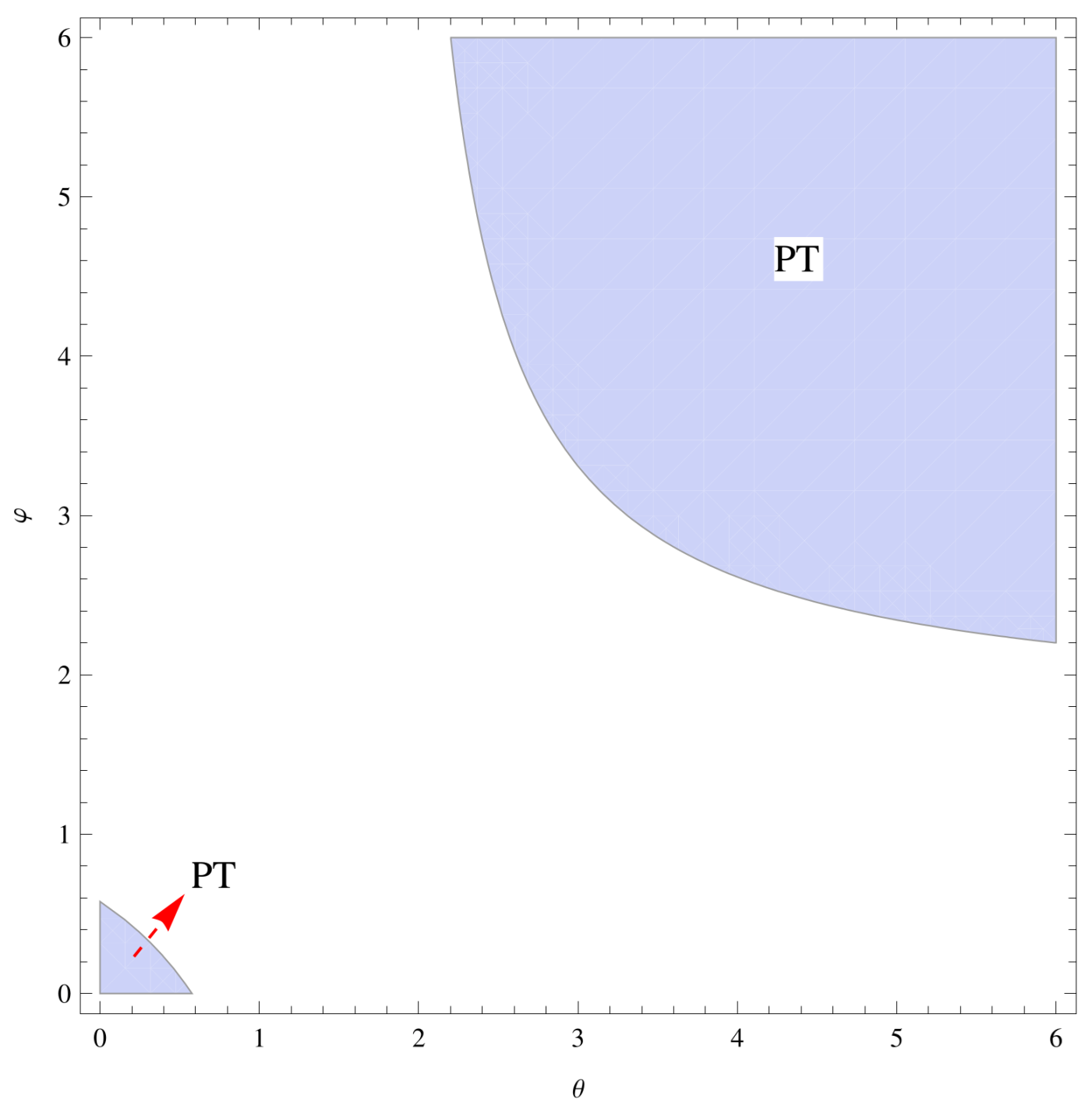
The blue region in Figure 3 represents the solution set of the inequality

$$\left(1-3{\theta }^2-4\theta \phi -3{\phi }^2+{\theta }^2{\phi }^2\right)>0.$$

Accordingly, while the phase transition is provided for the model in the blue regions of Figure 3, no phase transition phenomenon occurs in the white region of Figure 3.

4.2. Illustrative Examples

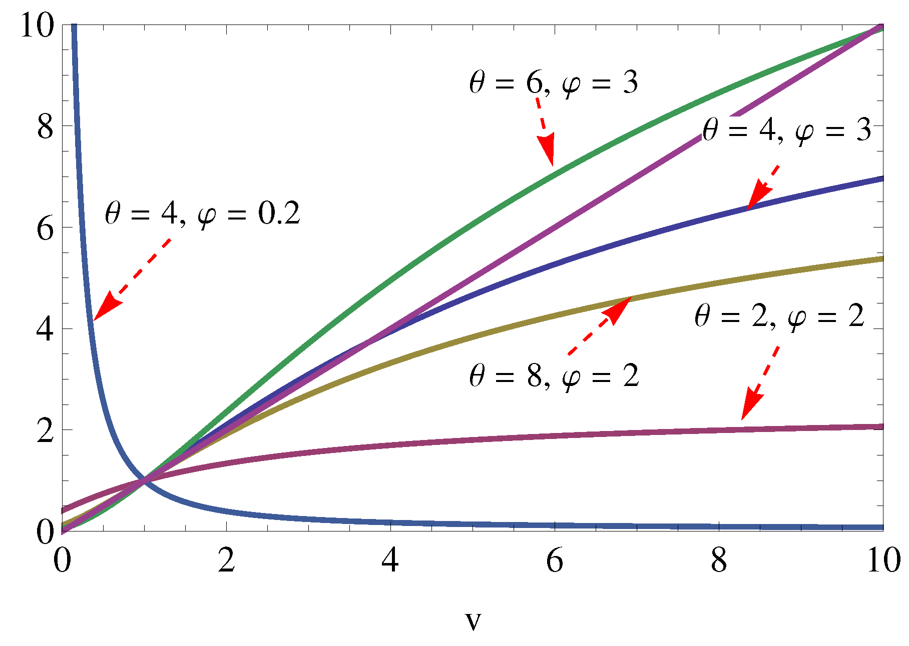
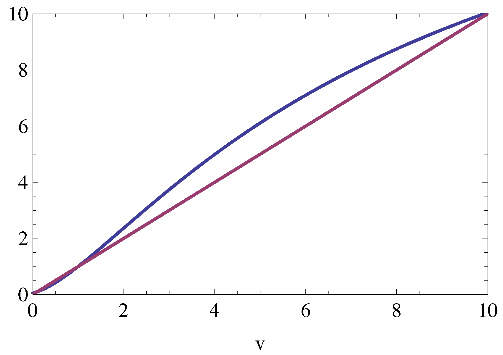
Figure 4 shows the graphs of the function $f_{\theta ,\phi }$ for given values of $\theta$ and $\phi$. For $(\theta =6, \phi =3)$ and $(\theta =4, \phi =3)$, the function $f_{\theta ,\phi }$ has three fixed points. For $(\theta =4, \phi =0.2)$, $(\theta =2, \phi =2)$ and $(\theta =8, \phi =2)$, the function $f_{\theta ,\phi }$ has a single fixed point.

The graph of the function $f_{\theta ,\phi }$ for $(\theta =0.2, \phi =0.3)$ is plotted in Figure 5. One can see that there are tree fixed points for $(\theta =0.2, \phi =0.3)$.

Note that each of these fixed points determines the limiting Gibbs measure associated with the model. As is known, if the number of the Gibbs measures corresponding to the model is more than one, then the phase transition is provided for the model. Therefore, from the Figure 4 and Figure 5, we can see that for $(\theta =6, \phi =3)$, $(\theta =4, \phi =3)$ and $(\theta =0.2, \phi =0.3)$, there are the phase transition. For $(\theta =4, \phi =0.2)$, $(\theta =2, \phi =2)$ and $(\theta =8, \phi =2)$, the phase transition does not occur.

5. Conclusions

In this elucidation, inspired by the results obtained for the one-dimensional Ising model, we have computed the partition function and then the free energy associated with the Ising model having the NN and PNNN interactions and external field on a two-order CT. We have obtained a formula for the free energy of the Ising model on the semi-infinite CT of order two. Considering the self-similarity method, we will derive the free energy and the entropy formulas for other lattice models on the semi-infinite CT, such as the Potts model, the SOS model in our next work.

The most interesting finding here is that the phase transition occurs when both J and $J_p$ are negative (in the anti-ferromagnetic case). For the Ising model with the same Hamiltonian, no phase transition has occurred in the anti-ferromagnetic regimes in previous studies (see [16,22]).

It is well known that the entropy of the model is computed by $S(\beta ,h)=-\frac{F(\beta ,h)}{dT}$ [10,14,15]. Using this formula, the entropy of our current model will be investigated in more detail in future studies. In addition, the phase transition types of the system will be determined by considering both the free energy formula and the entropy function.

References

- Mézard, M.; Parisi, G. The Bethe lattice spin glass revisited. Eur. Phys. J. B 2001, 20, 217–233. [Google Scholar] [CrossRef] [Green Version]
- Baxter, R.J. Exactly Solved Models in Statistical Mechanics; Academic Press: New York, NY, USA, 1982. [Google Scholar]
- Georgii, H.-O. Gibbs Measures and Phase Transitions; De Gruyter: Berlin, Germany, 1988. [Google Scholar]
- Rozikov, U.A. Gibbs Measures on Cayley Trees; World Scientific Publishing Company: Singapore, 2013. [Google Scholar]
- Akın, H. Phase diagrams of lattice models on Cayley tree and chandelier network: A review. Condens. Matter Phys. 2022, 25, 32501. [Google Scholar] [CrossRef]
- Ostilli, M. Cayley Trees and Bethe Lattices: A concise analysis for mathematicians and physicists. Phys. A 2012, 391, 3417–3423. [Google Scholar] [CrossRef] [Green Version]
- Moraal, H. Ising spin systems on Cayley tree-like lattices: Spontaneous magnetization and correlation functions far from the boundary. Phys. A 1978, 92, 305–314. [Google Scholar] [CrossRef]
- Akın, H. New Gibbs measures of the Ising model on a Cayley tree in the presence of triple effective local external fields. Phys. B 2022, 645, 414221. [Google Scholar] [CrossRef]
- Seino, M. The free energy of the random Ising model on the Bethe lattice. Phys. A 1992, 181, 233–242. [Google Scholar] [CrossRef]
- Gandolfo, D.; Rakhmatullaev, M.M.; Rozikov, U.A.; Ruiz, J. On free energies of the Ising model on the Cayley tree. J Stat. Phys. 2013, 150, 1201–1217. [Google Scholar] [CrossRef] [Green Version]
- Ganikhodjaev, N.; Akın, H.; Temir, S. Potts model with two competing binary interactions. Turk. J. Math. 2007, 31, 229–238. [Google Scholar]
- Bethe, H.A. Statistical theory of superlattices. Proc. Roy. Soc. London Ser. A 1935, 150, 552–575. [Google Scholar] [CrossRef] [Green Version]
- Yedidia, J.S.; Freeman, W.T.; Weiss, Y. Understanding belief propagation and its generalizations. In Exploring Artificial Intelligence in the New Millennium; Lakemeyer, G., Nebel, B., Eds.; Morgan Kaufmann: Burlington, MA, USA, 2003; pp. 239–269. [Google Scholar]
- Akın, H. A novel computational method of the free energy for an Ising model on Cayley tree of order three. Chin. J. Phys. 2022, 77, 2276–2287. [Google Scholar] [CrossRef]
- Mukhamedov, F.; Akın, H.; Khakimov, O. Gibbs measures and free energies of Ising-Vannimenus Model on the Cayley tree. J. Stat. Mech. 2017, 053208. [Google Scholar] [CrossRef]
- Akın, H. Gibbs measures with memory of length 2 on an arbitrary-order Cayley tree. Int. J. Mod. Phys. C 2018, 29, 1850016. [Google Scholar] [CrossRef] [Green Version]
- Akın, H. Gibbs measures of an Ising model with competing interactions on the triangular chandelier-lattice. Condens. Matter Phys. 2019, 22, 23002. [Google Scholar] [CrossRef]
- Akın, H.; Ulusoy, S. Limiting Gibbs measures of the q-state Potts model with competing interactions. Phys. B 2022, 640, 413944. [Google Scholar] [CrossRef]
- Akın, H.; Mukhamedov, F. Phase transition for the Ising model with mixed spins on a Cayley tree. J. Stat. Mech. 2022, 2022, 053204. [Google Scholar] [CrossRef]
- Peng, J.; Sandev, T.; Kocarev, L. First encounters on Bethe lattices and Cayley trees. Commun. Nonlinear Sci. Numer. Simul. 2021, 95, 105594. [Google Scholar] [CrossRef]
- Akın, H.; Temir, S. On phase transitions of the Potts model with three competing interactions on Cayley tree. Condens. Matter Phys. 2011, 14, 23003. [Google Scholar] [CrossRef] [Green Version]
- Akın, H. Determination of paramagnetic and ferromagnetic phases of an Ising model on a third-order Cayley tree. Condens. Matter Phys. 2021, 24, 13001. [Google Scholar] [CrossRef]
Figure 1.
(Color online) The image denotes a fourth-order Cayley tree having 4 shells (or levels) by , where O is the root vertex of . The region separated by dashed lines represents a third-order semi-finite Cayley tree with 3 shells and will be denoted by .
Figure 2.
(Color online) (a) A semi-ball with the center and radius 2 on the second-order CT. (b) Possible configurations that can be placed on the semi-ball given on the left.
Figure 3.
(Color online) The blue regions show the phase transition regimes for the model.
Figure 4.
(Color online) The graphs of the function for given values of and .
Figure 5.
(Color online) The graph of the function for .
Publisher’s Note: MDPI stays neutral with regard to jurisdictional claims in published maps and institutional affiliations. |
© 2022 by the author. Licensee MDPI, Basel, Switzerland. This article is an open access article distributed under the terms and conditions of the Creative Commons Attribution (CC BY) license (https://creativecommons.org/licenses/by/4.0/).
Share and Cite
MDPI and ACS Style
Akın, H. Calculation of the Free Energy of the Ising Model on a Cayley Tree via the Self-Similarity Method. Axioms 2022, 11, 703. https://doi.org/10.3390/axioms11120703
AMA Style
Akın H. Calculation of the Free Energy of the Ising Model on a Cayley Tree via the Self-Similarity Method. Axioms. 2022; 11(12):703. https://doi.org/10.3390/axioms11120703
Chicago/Turabian StyleAkın, Hasan. 2022. "Calculation of the Free Energy of the Ising Model on a Cayley Tree via the Self-Similarity Method" Axioms 11, no. 12: 703. https://doi.org/10.3390/axioms11120703
Note that from the first issue of 2016, this journal uses article numbers instead of page numbers. See further details here.